Controlled generation of momentum states in a high-finesse ring cavity

Abstract

A Bose-Einstein condensate in a high-finesse ring cavity scatters the photons of a pump beam into counterpropagating cavity modes, populating a bi-dimensional momentum lattice. A high-finesse ring cavity with a sub-recoil linewidth allows to control the quantized atomic motion, selecting particular discrete momentum states and generating atom-photon entanglement. The semiclassical and quantum model for the 2D collective atomic recoil lasing (CARL) are derived and the superradiant and good-cavity regimes discussed. For pump incidence perpendicular to the cavity axis, the momentum lattice is symmetrically populated. Conversely, for oblique pump incidence the motion along the two recoil directions is unbalanced and different momentum states can be populated on demand by tuning the pump frequency.

1 Introduction

Their unique coherence properties candidate Bose-Einstein condensates (BECs) as ideal systems to generate and probe light-atom correlations in collective light scattering and superradiant instabilities Yukalov . Superradiant Rayleigh scattering experiments usually occur in free space Inouye1999 ; Fallani2005 , so that scattered photons rapidly leave the interaction volume, limiting the coherence time of modes propagating along the major condensate’s axis (’end-fire modes’). On the contrary, when BECs interact with a high-finesse optical cavity, the correlations between scattered events can be stored in long-lived cavity modes SlamaPRL2007 , allowing, for instance, to study new regimes in the strong coupling limit Brennecke2007 ; Baumann2010 . Furthermore, recent experiments on collective light scattering by BECs in a high-finesse ring cavity have shown the possibility to employ the cavity sub-recoil resolution as a filter selecting particular quantized momentum states BuxPRL2011 . These experiments rely on the collective atomic recoil lasing (CARL) mechanism, envisaged by Bonifacio and coworker in 1994 CARL and finally observed in Tübingen, early with atomic clouds as hot as several $100\mu$K Kruse2003 and more recently with ultra-cold atoms SlamaPRA2007 . CARL represents the atomic analogue of the free-electron laser (FEL) Madey , which has been studied for a long time in Milan BPN ; NC . In particular, Bonifacio and Casagrande predicted the existence of a superradiant regime in FELs BC1984 ; BCJOSA1985 , successively observed as collective light scattering in CARL SlamaPRA2007 . A further advance on CARL theory was obtained in 2001, when the semiclassical model was extended to a quantum description suitable for BECs, in which the atomic motion is quantized in photon recoil momentum states Gatelli2001 ; Martinucci2002 . Next, a full quantum CARL theory investigated entanglement between collective momentum states and cavity modes Piovella2003 ; Cola2004 . Generally, CARL is often described in a 1D geometry, i.e. with pump and scattered modes anti-parallel and atoms recoiling after each scattering event by $2\hbar k$ along the incident beam direction. However, in the former Superradiant Rayleigh scattering experiment Inouye1999 the cigar-shaped condensate major axis was set orthogonal to the incident laser, and two scattered beams were emitted along the condensate axis, with atoms recoiling at 45^∘ with respect to the incident laser. In that case, the geometry was two-dimensional with two scattered end-fire modes. CARL and Superradiant Rayleigh scattering in a 2D configuration have been investigated by several authors Moore1999 ; Muste2000 ; Trifonov2001 ; PiovellaLP2002 ; PiovellaLP2003 ; Zobay2005 ; Zobay2006 ; Hilliard2008 ; Lu2011 . More recently, a two-frequency pumping scheme has been implemented to enhance the resonant sequential scattering in the Superradiant Rayleigh scattering BarGill2007 ; Yang2008 and in CARL ColaVolpe2009 . In particular, a sub-recoil cavity linewidth combined with a bi-chromatic pump, with frequency separated by twice the recoil frequency, allows to observe subradiance in a degenerate cascade between three collective momentum states ColaBigerni2009 .

In this paper I consider a BEC in a high-finesse ring cavity scattering photons from a pump beam into two counter-propagating cavity modes BuxPRL2011 . Varying the pump intensity and frequency, it is possible to populate in a controlled way a 2D momentum lattice, where atoms belonging to different sites get entangled with the scattered cavity photons. The paper is organized as follow: In sec.II I derive the semiclassical 2D CARL model for a pump beam incident at variable angle; In sec.III the atomic motion is quantized. Sec. IV discusses the different quantum regimes and present some numerical result in the nonlinear regime.

2 Semiclassical model

Let’s consider $N$ two-level atoms (with $|a\rangle$ and $|b\rangle$ upper and lower states, respectively) in a cloud with length $L$ and diameter $W\ll L$, exposed to an uniform, $s$-polarized along $\hat{\mathbf{e}}_{y}$ laser beam, incident in the cavity plane $(x,z)$ and making an angle $\phi$ respect to the normal of the cavity’s optical axis $z$ (see fig.1), with electric field

$$\mathbf{E}_{i}=\frac{\hat{\mathbf{e}}_{y}}{2}\left\{E_{0}e^{i(k_{0}x\cos\phi-k_{0}z\sin\phi-\omega_{0}t)}+\textrm{c.c.}\right\}$$ (1)

with $\omega_{0}=ck_{0}$. The pump photons are scattered in two counter-propagating cavity modes with frequency coinciding with a cavity eigenfrequency, $\omega_{c}=ck_{c}$, and electric field

$$\mathbf{E}_{s}=\frac{\hat{\mathbf{e}}_{y}}{2}\left\{E_{1}e^{i(k_{c}z-\omega_{c}t)}+E_{2}e^{-i(k_{c}z+\omega_{c}t)}+\textrm{c.c.}\right\}$$ (2)

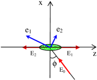
Figure 1: 2D CARL configuration: the pump field $E_{0}$ is incident with an angle $\phi$ with respect to the normal of the cavity axis $\hat{z}$, and the cavity modes $E_{1}$ and $E_{2}$ are counter-propagating along $\hat{z}$. All the fields are linearly polarized perpendicularly to the cavity plane. The atoms recoil along the $\hat{\mathbf{e}}_{1}$ and $\hat{\mathbf{e}}_{2}$ directions, when they scatter $E_{0}$ pump photons into the modes $E_{1}$ or $E_{2}$, respectively.

The pump and the two cavity mode fields induce the following coherence between the states $|a\rangle$ and $|b\rangle$,

$$\rho_{ab}=\frac{1}{2}\left\{S_{0}e^{ik_{0}(x\cos\phi-z\sin\phi-ct)}+S_{1}e^{ik_{c}(z-ct)}+S_{2}e^{-ik_{c}(z+ct)}+\textrm{c.c.}\right\}$$ (3)

and a force $\mathbf{F}=d_{y}\mathbf{\nabla}(\mathbf{E}_{i}+\mathbf{E}_{s})_{y}$ in the cavity plane $(x,z)$, where $d_{y}=d(\rho_{ab}+\textrm{c.c.})$ is the $y$-component of the electric dipole moment and $d$ is the dipole matrix element. Assuming the pump-atom detuning $\Delta_{a}=\omega_{0}-\omega_{a}$ much larger than the spontaneous decay rate $\Gamma$, it is possible to see that $S_{i}\approx-\Omega_{i}/\Delta_{a}$ (for $i=0,1,2$), where $\Omega_{i}=dE_{i}/\hbar$ CARL . A straightforward calculation shows that the equations for the momentum components $p_{x,z}=mv_{x,z}$ are PiovellaLP2003

$$\frac{dp_{x}}{dt} = i\frac{\hbar k_{0}\Omega_{0}}{4\Delta_{a}}\cos\phi\left\{\tilde{\Omega}_{1}e^{-i\mathbf{q}_{1}\cdot\mathbf{x}}+\tilde{\Omega}_{2}e^{-i\mathbf{q}_{2}\cdot\mathbf{x}}-\textrm{c.c.}\right\}$$ (4)

$$\frac{dp_{z}}{dt} = -i\frac{\hbar k_{0}\Omega_{0}}{4\Delta_{a}}\sin\phi\left\{\tilde{\Omega}_{1}e^{-i\mathbf{q}_{1}\cdot\mathbf{x}}-\tilde{\Omega}_{2}e^{-i\mathbf{q}_{2}\cdot\mathbf{x}}-\textrm{c.c.}\right\}-i\frac{\hbar k_{0}\Omega_{0}}{4\Delta_{a}}\left\{\tilde{\Omega}_{1}e^{-i\mathbf{q}_{1}\cdot\mathbf{x}}-\tilde{\Omega}_{2}e^{-i\mathbf{q}_{2}\cdot\mathbf{x}}-\textrm{c.c.}\right\}$$ (5)

$$- i\frac{\hbar k_{0}}{2\Delta_{a}}\left\{\tilde{\Omega}_{1}\tilde{\Omega}_{2}^{*}e^{2ik_{0}z}-\textrm{c.c.}\right\}$$

where we assumed $k_{c}\sim k_{0}$, we introduced $\tilde{\Omega}_{1,2}=\Omega_{1,2}\exp(i\Delta_{c}t)$, where $\Delta_{c}=\omega_{0}-\omega_{c}$ is the pump-cavity detuning, and

$$\mathbf{q}_{1,2}=k_{0}[\cos\phi\,\hat{\mathbf{e}}_{x}-(\sin\phi\pm 1)\hat{\mathbf{e}}_{z}],$$ (6)

where $\mathbf{q}_{1}\cdot\mathbf{q}_{2}=0$. The equations for the cavity mode amplitudes are

$$\frac{d\tilde{\Omega}_{1}}{dt} = \frac{ck_{0}d^{2}n_{a}}{2i\epsilon_{0}\hbar\Delta_{a}}\left\{\Omega_{0}\langle e^{i\mathbf{q}_{1}\cdot\mathbf{x}}\rangle+\tilde{\Omega}_{1}+\tilde{\Omega}_{2}\langle e^{-2ik_{0}z}\rangle\right\}-\kappa_{c}\tilde{\Omega}_{1}+i\Delta_{c}\tilde{\Omega}_{1}$$ (7)

$$\frac{d\tilde{\Omega}_{2}}{dt} = \frac{ck_{0}d^{2}n_{a}}{2i\epsilon_{0}\hbar\Delta_{a}}\left\{\Omega_{0}\langle e^{i\mathbf{q}_{2}\cdot\mathbf{x}}\rangle+\tilde{\Omega}_{2}+\tilde{\Omega}_{1}\langle e^{2ik_{0}z}\rangle\right\}-\kappa_{c}\tilde{\Omega}_{2}+i\Delta_{c}\tilde{\Omega}_{2}$$ (8)

where $n_{a}$ is the atomic density and $\kappa_{c}=c{\cal{T}}/L_{c}$ is the linewidth of the ring cavity with length $L_{c}$ and transmission $\cal{T}$. It is more convenient to describe the atomic motion along the directions of $\mathbf{q}_{1,2}=q_{1,2}\hat{\mathbf{e}}_{1,2}$ with unitary vectors $\hat{\mathbf{e}}_{1,2}$ and $q_{1,2}=k_{0}\sqrt{2(1\pm\sin\phi)}$. Then, the momentum components along these directions are, in units of the photon recoil momentum $\hbar q_{1,2}$,

$$p_{1,2}=\frac{\mathbf{p}\cdot\hat{\mathbf{e}}_{1,2}}{\hbar q_{1,2}}=\frac{k_{0}}{\hbar q_{1,2}^{2}}\left[p_{x}\cos\phi-p_{z}(\sin\phi\pm 1)\right].$$ (9)

Defining the phases

$$\theta_{1,2}=\mathbf{q}_{1,2}\cdot\mathbf{x}=k_{0}x\cos\phi-k_{0}z(\sin\phi\pm 1)$$ (10)

and the dimensionless field amplitudes

$$a_{1,2}=i\sqrt{\frac{\epsilon_{0}\hbar V}{2d^{2}\omega_{0}}}\tilde{\Omega}_{1,2}=i\sqrt{\frac{\epsilon_{0}V}{2\hbar\omega_{0}}}E_{1,2}e^{i\Delta_{c}t}$$ (11)

where $V$ is the interaction volume, the complete equations for $N$ atoms and the two cavity mode amplitudes are

$$\frac{d\theta_{1j}}{dt} = 2\omega_{r1}p_{1j}$$ (12)

$$\frac{d\theta_{2j}}{dt} = 2\omega_{r2}p_{2j}$$ (13)

$$\frac{dp_{1j}}{dt} = \frac{g\Omega_{0}}{2\Delta_{a}}\left\{a_{1}e^{-i\theta_{1j}}+\textrm{c.c.}\right\}+i\frac{g^{2}}{\Delta_{a}}\left\{a_{1}a_{2}^{*}e^{i(\theta_{2j}-\theta_{1j})}-\textrm{c.c}.\right\}$$ (14)

$$\frac{dp_{2j}}{dt} = \frac{g\Omega_{0}}{2\Delta_{a}}\left\{a_{2}e^{-i\theta_{2j}}+\textrm{c.c.}\right\}-i\frac{g^{2}}{\Delta_{a}}\left\{a_{1}a_{2}^{*}e^{i(\theta_{2j}-\theta_{1j})}-\textrm{c.c.}\right\}$$ (15)

$$\frac{da_{1}}{dt} = \frac{Ng\Omega_{0}}{2\Delta_{a}}\langle e^{i\theta_{1}}\rangle-i\frac{Ng^{2}}{2\Delta_{a}}a_{2}\langle e^{-i(\theta_{2}-\theta_{1})}\rangle-\kappa_{c}a_{1}+i\left(\Delta_{c}-\frac{Ng^{2}}{\Delta_{a}}\right)a_{1}$$ (16)

$$\frac{da_{2}}{dt} = \frac{Ng\Omega_{0}}{2\Delta_{a}}\langle e^{i\theta_{2}}\rangle-i\frac{Ng^{2}}{2\Delta_{a}}a_{1}\langle e^{i(\theta_{2}-\theta_{1})}\rangle-\kappa_{c}a_{2}+i\left(\Delta_{c}-\frac{Ng^{2}}{\Delta_{a}}\right)a_{2}$$ (17)

where $j=1,\dots,N$, $g=\sqrt{d^{2}\omega_{0}/(2\epsilon_{0}\hbar V)}$ is the single-photon Rabi frequency and

$$\omega_{r1,2}=\frac{1}{2}\left(1\pm\sin\phi\right)\omega_{r},$$ (18)

where $\omega_{r}=2\hbar k_{0}^{2}/m$ is the maximum photon recoil frequency. Notice that the atoms move along the recoiling directions $\hat{\mathbf{e}}_{1}$ or $\hat{\mathbf{e}}_{2}$ (see fig.1) when they scatter the pump photons into the cavity modes $a_{1}$ and $a_{2}$, respectively (see the first terms on the right hand sides of Eqs.(14) and (15), representing the dipole forces depending on $\theta_{1j}$ and $\theta_{2j}$, respectively). Furthermore, the atoms recoil further along the cavity axis $\hat{z}$ when they exchange photons between the two cavity modes themselves (see the second terms on the right hand sides of Eqs.(14) and (15), representing the dipole force due to the two-cavity mode interference and depending on $\theta_{2j}-\theta_{1j}=2k_{0}z_{j}$). Notice that the longitudinal dipole force breaks the pump-atom detuning $\Delta_{a}$ symmetry: In fact, if $\Delta_{a}\rightarrow-\Delta_{a}$ and $a_{1,2}\rightarrow-a_{1,2}$, these terms change sign too (together with the collective single-photon light shift $Ng^{2}/\Delta_{a}$).

3 Quantum model

In a quantum theory, the classical variables $\theta_{1j}$, $\theta_{2j}$, $p_{1j}$, $p_{2j}$, $a_{1}$ and $a_{2}$ are promote to operators, with commutation rules $[\theta_{\alpha j},p_{\beta m}]=i\delta_{\alpha\beta}\delta_{jm}$ and $[a_{\alpha},a_{\beta}^{\dagger}]=\delta_{\alpha\beta}$ where $\alpha,\beta=1,2$. Without cavity losses (i.e. $\kappa_{c}=0$), Eqs.(12)-(17) derive by the following Hamiltonian:

$$H = \sum_{j=1}^{N}\left\{\omega_{r1}p_{1j}^{2}+\omega_{r2}p_{2j}^{2}+i\frac{g\Omega_{0}}{2\Delta_{a}}\left[a_{1}^{\dagger}e^{i\theta_{1j}}+a_{2}^{\dagger}e^{i\theta_{2j}}-\textrm{h.c.}\right]+\frac{g^{2}}{\Delta_{a}}\left[a_{1}a_{2}^{\dagger}e^{i(\theta_{2j}-\theta_{1j})}+\textrm{h.c.}\right]\right\}$$ (19)

$$- \left(\Delta_{c}-\frac{Ng^{2}}{\Delta_{a}}\right)(a_{1}^{\dagger}a_{1}+a_{2}^{\dagger}a_{2}).$$

The single-particle Hamiltonian $H_{1}(\theta_{1},\theta_{2},p_{1},p_{2},a_{1},a_{1}^{\dagger},a_{2},a_{2}^{\dagger})$ can be second-quantized as

$$\hat{H} = \int_{0}^{2\pi}d\theta_{1}\int_{0}^{2\pi}d\theta_{2}\hat{\Psi}^{\dagger}(\theta_{1},\theta_{2})H_{1}(\theta_{1},\theta_{2},-i\partial_{\theta_{1}},-i\partial_{\theta_{2}},a_{1},a_{1}^{\dagger},a_{2},a_{2}^{\dagger})\,\hat{\Psi}(\theta_{1},\theta_{2})\quad\quad$$ (20)

where the quantum field operator $\hat{\Psi}(\theta_{1},\theta_{2})$ obeys bosonic equal-time commutation rules $[\hat{\Psi}(\theta_{1},\theta_{2}),\hat{\Psi}^{\dagger}(\theta_{1}^{\prime},\theta_{2}^{\prime})]=\delta(\theta_{1}-\theta_{1}^{\prime})\delta(\theta_{2}-\theta_{2}^{\prime})$ and $[\hat{\Psi}(\theta_{1},\theta_{2}),\hat{\Psi}(\theta_{1}^{\prime},\theta_{2}^{\prime})]=0$, with normalization condition $\int d\theta_{1}\int d\theta_{2}\hat{\Psi}^{\dagger}(\theta_{1},\theta_{2})\hat{\Psi}(\theta_{1},\theta_{2})=\hat{N}$. Introducing the annihilation operators for the two momentum components $p_{1}$ and $p_{2}$, i.e. $\hat{\Psi}(\theta_{1},\theta_{2})=\sum_{m,n}\hat{c}_{m,n}u_{m}(\theta_{1})u_{n}(\theta_{2})$, where $u_{m}(\theta_{1,2})=(1/\sqrt{2\pi})\exp[im\theta_{1,2}]$ and $[\hat{c}_{m,n},\hat{c}_{m^{\prime},n^{\prime}}^{\dagger}]=\delta_{m,m^{\prime}}\delta_{n,n^{\prime}}$, the Heisenberg equations for $\hat{c}_{m,n}$, $\hat{a}_{1}$ and $\hat{a}_{2}$ read:

$$\frac{d\hat{c}_{m,n}}{dt} = -i\left[m^{2}\omega_{r1}+n^{2}\omega_{r2}\right]\hat{c}_{m,n}$$ (21)

$$+ \frac{g\Omega_{0}}{2\Delta_{a}}\left[\hat{a}_{1}^{\dagger}\hat{c}_{m-1,n}+\hat{a}_{2}^{\dagger}\hat{c}_{m,n-1}-\hat{a}_{1}\hat{c}_{m+1,n}-\hat{a}_{2}\hat{c}_{m,n+1}\right]$$

$$- i\frac{g^{2}}{\Delta_{a}}\left[a_{1}a_{2}^{\dagger}\hat{c}_{m+1,n-1}+a_{1}^{\dagger}a_{2}\hat{c}_{m-1,n+1}\right]$$

$$\frac{d\hat{a}_{1}}{dt} = \frac{g\Omega_{0}}{2\Delta_{a}}\sum_{m,n}\hat{c}^{\dagger}_{m,n}\hat{c}_{m-1,n}-i\frac{g^{2}}{\Delta_{a}}\hat{a}_{2}\sum_{m,n}\hat{c}_{m,n}^{\dagger}\hat{c}_{m-1,n+1}+i\Delta\hat{a}_{1}$$ (22)

$$\frac{d\hat{a}_{2}}{dt} = \frac{g\Omega_{0}}{2\Delta_{a}}\sum_{m,n}\hat{c}^{\dagger}_{m,n}\hat{c}_{m,n-1}-i\frac{g^{2}}{\Delta_{a}}\hat{a}_{1}\sum_{m,n}\hat{c}_{m,n}^{\dagger}\hat{c}_{m+1,n-1}+i\Delta a_{2}$$ (23)

where $\Delta=\Delta_{c}-Ng^{2}/\Delta_{a}$. Notice that in Eq.(21) we have neglected the global phase factor proportional to $\Delta(a_{1}^{\dagger}a_{1}+a_{2}^{\dagger}a_{2})$.

In the following we will neglect the quantum nature of the operators $\hat{c}_{m,n}$ and $\hat{a}_{1,2}$ and we treat them as complex dynamical variables. Furthermore, we introduce dimensionless time, $\tau=2\omega_{r}\rho t$, field amplitudes, $A_{1,2}=(a_{1,2}/\sqrt{\rho N})\exp(-i\Delta t)$, and pump parameter, $A_{0}=a_{0}/\sqrt{\rho N}$, where $a_{0}=\Omega_{0}/(2g)$ is such that $a_{0}^{2}$ is the pump photon number. The collective CARL parameter $\rho$ is defined as CARL

$$\rho=\left(\frac{a_{0}g^{2}\sqrt{N}}{2\Delta_{a}\omega_{r}}\right)^{2/3},$$ (24)

Then, defining $C_{m,n}=(1/\sqrt{N})c_{m,n}\exp[i(m+n)\Delta t]$, $\kappa=\kappa_{c}/(2\omega_{r}\rho)$ and $\delta=\Delta/\omega_{r}$, Eqs.(21)-(23) yield

$$\frac{dC_{m,n}}{d\tau} = -\frac{i}{2\rho}\left[m^{2}\left(\frac{1+\sin\phi}{2}\right)+n^{2}\left(\frac{1-\sin\phi}{2}\right)-(m+n)\delta\right]C_{m,n}$$ (25)

$$+ \rho\left[A_{1}^{*}C_{m-1,n}+A_{2}^{*}C_{m,n-1}-A_{1}C_{m+1,n}-A_{2}C_{m,n+1}\right]$$

$$- i\frac{\rho}{A_{0}}\left[A_{1}A_{2}^{*}C_{m+1,n-1}+A_{1}^{*}A_{2}C_{m-1,n+1}\right]$$

$$\frac{dA_{1}}{d\tau} = \sum_{m,n}C^{*}_{m,n}C_{m-1,n}-i\frac{A_{2}}{A_{0}}\sum_{m,n}C_{m,n}^{*}C_{m-1,n+1}-\kappa A_{1}$$ (26)

$$\frac{dA_{2}}{d\tau} = \sum_{m,n}C^{*}_{m,n}C_{m,n-1}-i\frac{A_{1}}{A_{0}}\sum_{m,n}C_{m,n}^{*}C_{m+1,n-1}-\kappa A_{2}$$ (27)

Notice that the total probability is conserved, i.e. $\sum_{m,n}|C_{m,n}|^{2}=1$. The growth rates for the two modes are $G_{1,2}=-2\textrm{Im}(\lambda)(2\omega_{r}\rho)$, where $\lambda$ is the solution of the cubic dispersion relation:

$$\left(\lambda-\frac{\delta}{2\rho}-i\kappa\right)\left[\lambda^{2}-\left(\frac{s_{1,2}}{2\rho}\right)^{2}\right]+s_{1,2}=0,$$ (28)

where $s_{1,2}=(1\pm\sin\phi)/2$. Notice that the longitudinal lattice term is nonlinear (being proportional to $A_{1}A_{2}^{*}$) and it does not contribute to the dispersion relation (28). In the following we will indicate the 2D momentum lattice states as $(m,n)$, associated with momentum components $\mathbf{p}_{1}=m(\hbar q_{1})\hat{\mathbf{e}}_{1}$ and $\mathbf{p}_{2}=m(\hbar q_{2})\hat{\mathbf{e}}_{2}$, respectively. In the linear regime, the two cavity modes grow independently and atoms (initially in $(0,0)$) populate the states $(\pm 1,0)$ and $(0,\pm 1)$, respectively. In particular, when the laser beam is parallel to the cavity axis $\hat{z}$ (i.e. $\phi=90^{\circ}$), $s_{1}=1$ and $s_{2}=0$: Only the mode $a_{1}$ grows, so we can set $a_{2}=0$ and the model reduces to the usual 1D CARL, with $c_{m,n}=\delta_{n,0}c_{m}$ Gatelli2001 .

4 Discussion

After scattered a photon with momentum $\hbar\mathbf{k}$ and energy $\hbar\omega$, the atom recoils with momentum $\mathbf{p}$ determined by energy and momentum conservation laws, i.e. $\hbar\mathbf{k}_{0}=\hbar\mathbf{k}+\mathbf{p}$ and $\hbar\omega_{0}=\hbar\omega+p^{2}/2m$, so that $p_{x}=\hbar k_{0}\cos\phi$, $p_{z}=\hbar k_{0}(\sin\phi\mp 1)$ and $\omega=\omega_{0}-\omega_{r}(1\pm\sin\phi)/2$, where the upper and lower sign is for a photon emitted in the cavity mode $a_{1}$ or $a_{2}$, respectively. Since $\omega$ is near the cavity mode frequency $\omega_{c}$, then by tuning the pump frequency $\omega_{0}$ near the cavity mode frequency $\omega_{c}$ it is possible to enhance one mode with respect to the other, depending on incidence angle $\phi$, gain bandwidth $\omega_{r}\rho$ and cavity linewidth $\kappa_{c}$ values BuxPRL2011 .

4.1 ’Good-Cavity’ and ’Superradiant’ regimes

The cubic dispersion relation (28) provides the expression for the gain rates $G_{1,2}$ of the two cavity modes in the good-cavity (GC) regime (i.e. when $2\kappa_{c}\ll G_{1,2}$) and in the super-radiant (SR) regime (i.e. when $2\kappa_{c}\geq G_{1,2}$), either in the semiclassical regime (i.e. when $\Delta\omega\gg\omega_{r}$) or in the quantum regime (i.e. when $\Delta\omega\leq\omega_{r}$), where $\Delta\omega$ is the resonant gain bandwidth Gatelli2001 ; Martinucci2002 ; Piovella2003 . In particular, in the quantum regime the atoms scatter the pump scattered photons only forward, since the atomic recoil red-shifts the scattered photon frequency (i.e. at $\omega-\omega_{r1,2}$) such that it is set out of the resonant gain bandwidth Gatelli2001 . So, in the quantum regime the atoms populate initially only the positive-momentum states $(1,0)$ and $(0,1)$. In the GC limit we can set $\kappa_{c}=0$, obtaining $G_{1,2}=2\sqrt{(2\rho)^{3}\omega_{r}^{2}-\Delta_{1,2}^{2}}$ for $\Delta_{1,2}<(2\rho)^{3/2}\omega_{r}$, where $\Delta_{1,2}=\Delta-\omega_{r1,2}$ is the detuning taking into account the recoil shift. Hence, in the quantum GC regime, the maximum gain and the gain bandwidth are $G_{max}=2(2\rho)^{3/2}\omega_{r}$ and $\Delta\omega=2(2\rho)^{3/2}\omega_{r}=G_{max}$, respectively, and the conditions necessary to observe it are $\rho<1$ and $\kappa_{c}\ll\omega_{r}$. In the quantum SR regime, $G_{1,2}=\kappa_{c}(2\omega_{r}\rho)^{2}/(\Delta_{1,2}^{2}+\kappa_{c}^{2})$, so that the maximum gain is $G_{max}=(2\omega_{r}\rho)^{2}/\kappa_{c}$ and the gain bandwidth is $\kappa_{c}$ Martinucci2002 . The condition necessary to observe the quantum SR regime is $\omega_{r}\rho\leq\kappa_{c}<\omega_{r}$. Notice that in the quantum regime gain and bandwidth are the same for the two modes. However, increasing $\rho$ for a given cavity linewidth $\kappa_{c}$, the system moves toward the classical GC limit, $G_{1,2}\gg\omega_{r}$, where the recoil shift can be neglected and the gain is centered around $\Delta=0$, with $G_{max}=2\sqrt{3}\,\omega_{r}\rho(s_{1,2})^{1/3}$. Hence, in the classical regime the two cavity modes have different gain rates. As an example of an intermediate case (with parameters close to those of ref.BuxPRL2011 ), fig.2 shows the gain $G_{1,2}$ (in CARL bandwidth $2\rho\omega_{r}$ units) vs. the pump cavity detuning $\delta=\Delta/\omega_{r}$, for $\phi=45^{\circ}$, $\rho=0.4$ and $\kappa_{c}=0.8\omega_{r}$.

Figure 2: Gain coefficients $g_{1,2}=-2Im(\lambda)$ (continuous blue line for mode $1$ and dashed red line for mode $2$) vs. the pump-cavity detuning $\delta=\Delta/\omega_{r}$, for $\phi=45^{\circ}$, $\rho=0.4$ and $\kappa_{c}=0.8\omega_{r}$.

4.2 Symmetric nonlinear regime

The case where the laser beam is perpendicular to the cavity axis $\hat{z}$ (i.e. $\phi=0$ and $s_{1,2}=1/2$) has been discussed in details in ref.PiovellaLP2003 . Here, the two modes are symmetric and atoms move at $45^{\circ}$ forward and backward with respect to the cavity axis. This is also the original configuration of the Superradiant Rayleigh scattering experiment of ref.Inouye1999 . Following ref.PiovellaLP2003 , it results that in the quantum regime atoms populate sequentially the momentum states $(n,n)$ (with $n=1,2,\dots$) by a four-level ’diamond’ transition, passing through the intermediate states $(n-1,n)$ and $(n,n-1)$. Since $c_{n,m}=c_{m,n}$ and $A_{1}=A_{2}$, each transition $(n-1,n-1)\rightarrow(n,n)$ can be described by optical Bloch equations for two-level systems once a population difference $W=|c_{n-1,n-1}|^{2}-|c_{n,n}|^{2}$ and a polarization $S=c_{n-1,n-1}^{*}c_{n-1,n}+c_{n-1,n}^{*}c_{n,n}$ are introduced. In the quantum SR regime and at resonance (i.e. for $\Delta=\omega_{r}/2$), the populations evolve as $|c_{n,n}(\tau)|^{2}=(1/4)\left\{1-\tanh[\sqrt{\rho/\kappa}(\tau-\tau_{D})]\right\}^{2}$ and $|c_{n-1,n}(\tau)|^{2}=(1/4)\textrm{sech}^{2}[\sqrt{\rho/\kappa}(\tau-\tau_{D})]$, whereas the cavity photon number is $\langle n_{ph}\rangle=N\textrm{sech}^{2}[\sqrt{\rho/\kappa}(\tau-\tau_{D})]$, where $\tau_{D}\approx\sqrt{\rho}\ln(\rho)$. Notice that the maximum occupation probability of the intermediate states $(n-1,n)$ and $(n,n-1)$ is $1/4$. This configuration is particular attractive, since either entanglement Porras2008 and subradiance could be there easily addressed, as discussed by Crubellier et al. Crubellier1985 ; Crubellier1986 .

4.3 Asymmetric nonlinear regime

The symmetry of the case with perpendicular incidence is broken when the laser beam shines the atoms with an oblique incidence angle, as can be seen for instance in fig.1. In this case, changing the laser frequency $\omega_{0}$ with respect to the cavity mode frequency $\omega_{c}$ allows to unbalance the two counter-propagating cavity modes, as well as the two momentum components $p_{1}$ and $p_{2}$. Furthermore, nonlinearity induces more complicated dynamical structures resulting from the interplay of cooperative gain and cavity losses, when more than one photon is scattered by the condensate. As an example, we consider the case with $\phi=45^{\circ}$, $\rho=0.4$, $\kappa=0.8\omega_{r}$ and different pump-cavity detuning $\Delta$. In order to ge the analysis simpler, we neglect the longitudinal lattice (i.e. the last term in the right-hand side of Eqs.(25) and the second terms in the right-hand side of Eqs.(26) and (27)) assuming $A_{1,2}\ll A_{0}$. Fig.3 shows the result of numerical integration of Eqs.(25)-(27) for different pump-cavity detuning values: $\Delta=-2.5\omega_{r}$ (left column), $\Delta=-0.025\omega_{r}$ (central column) and $\Delta=2\omega_{r}$ (right column); mode intensities $|A_{1,2}|^{2}$ and the average momentum components $\langle p_{1,2}\rangle$ are shown vs. $\tau$ in the upper and lower lines, respectively; blue thick lines refer to mode $1$ and red thin lines refer to mode $2$.

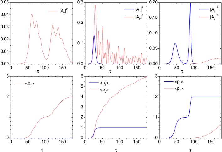
Figure 3: $|A_{1,2}|^{2}$ (upper line) and $\langle p_{1,2}\rangle$ (lower line) vs. dimensionless time $\tau$ for $\Delta=-2.5\omega_{r}$ (left column), $\Delta=-0.025\omega_{r}$ (central column) and $\Delta=2\omega_{r}$ (right column), for $\phi=45^{\circ}$, $\rho=0.4$ and $\kappa_{c}=0.8\omega_{r}$. Blue thick lines are for the mode $1$, red thin lines for the mode $2$.

For $\Delta=-2.5\omega_{r}$ (left column) $G_{1}\ll G_{2}$, so that the mode $1$ does not grow appreciably. The atoms move along the $\hat{\mathbf{e}}_{2}$ direction, up to the momentum state $(0,2)$ after a time $\tau=180$. For $\Delta=-0.025\omega_{r}$ (central column) the gain rates are equal ($G_{1}=G_{2}=0.41\omega_{r}$) and the atoms initially equally populate the momentum states $(1,0)$ and $(0,1)$. However, later on the atoms turn toward the $\hat{\mathbf{e}}_{2}$ direction, populating the states $(1,m)$ with $m=1,\dots,6$ after a time $\tau=180$. This rather peculiar behavior has been observed also in the experiment of ref.BuxPRL2011 . This behavior can be easily understood observing that the recoil shift for the mode $1$ is $s_{1}/s_{2}=5.83$ times larger than for the mode $2$, so that the incident photons are set out of resonance after the atoms have scattered the first laser photon into the mode $1$, whereas the incident photons remain well inside the resonant gain bandwidth when scattered into the mode $2$ (see fig.2). As a consequence, the atoms scatter a single photon into the mode $1$, stopping at the momentum states $(m,n)$ with $m=1$, whereas they are allowed to scatter photons into the mode $2$ (up to $n=6$, as shown in central column of fig.3), populating the momentum states $(1,n)$. Finally, for $\Delta=2\omega_{r}$ (right column of fig.3)) $G_{2}\ll G_{1}$, so initially only the mode $1$ grows and atoms populate sequentially the states $(1,0)$ and $(2,0)$; however, at a longer time the mode $2$ grows and reaches saturation, so that the atoms populate also the state $(2,1)$.

5 Conclusions

I have derived the semiclassical and quantum model of the collective atomic recoil laser (CARL) for a Bose-Einstein condensate set in an arm of an high-finesse ring cavity, with a laser beam incident at an oblique angle with respect to the cavity axis. The atoms scatter photons into two counterpropagating cavity modes, recoiling along two different directions determined by the incidence angle. For perpendicular incidence, atoms scatter symmetrically the pump photons into the two cavity modes, populating sequentially symmetric momentum states $(n,n)$ with $n=1,2,\dots$. Conversely, for oblique incidence it is possible to populate in a controlled way different momentum states by tuning the pump frequency, as experimentally done in ref.BuxPRL2011 . Similarly to the 1D geometry Piovella2003 ; Cola2004 , it is expected that atoms belonging to different momentum states may be entangled between themselves and/or with the photons scattered in the cavity modes. Furthermore, an even reacher scenario can be realized by a bichromatic pump with frequency spacing tuned around the recoil frequency, which is expected to enhance or inhibit the transfer of atoms between different momentum states ColaVolpe2009 ; ColaBigerni2009 .

6 Acknowledgments

This work is dedicated to Federico Casagrande, in memory of our long-standing friendship and of his unforgettable kindness and sympathy. I would like to thank Simone Bux, Philippe W. Courteille and Claus Zimmermann for helpful discussions about the experiment described in ref.BuxPRL2011 . This work has been supported by the Research Executive Agency (program COSCALI No. PIRSES-GA-2010-268717).

References

- (1) Ph.W. Courteille, V.S. Bagnato, V.I Yukalov, Laser Phys. 11, (2001) 659
- (2) S. Inouye, A.M. Chikkatur, D.M. Stamper-Kurn, et al., Science 285, (1999) 571
- (3) L. Fallani, C. Fort, N. Piovella, M. M. Cola, F. S. Cataliotti, M. Inguscio, R. Bonifacio Phys. Rev. A 71, (2005) 033612
- (4) S. Slama, S. Bux, G. Krenz, C. Zimmermann, Ph. W. Courteille, Phys. Rev. Lett. 98, (2007) 053603
- (5) F. Brennecke et al., Nature (London) 450, (2007) 268
- (6) K. Baumann et al., Nature (London) 464, (2010) 1301
- (7) S. Bux, C. Gnahm, R.A.W. Maier, C. Zimmermann, Ph. W. Courteille, Phys. Rev. Lett. 106, (2011) 203601
- (8) R. Bonifacio, L. De Salvo Souza, Nucl. Instrum. Methods Phys. Res. A 341, (1994) 360
- (9) Ch. von Cube, C. Zimmermann, Ph.W. Courteille, Phys. Rev. Lett. 91, (2003) 183601
- (10) S. Slama, G. Krenz, S. Bux, C. Zimmermann, Ph. W. Courteille, Phys. Rev. A 75, (2007) 063620
- (11) J. Madey, J. Appl. Phys. 42, (1971) 1906
- (12) R. Bonifacio, C. Pellegrini, L. Narducci, Opt. Commun. 50, (1984) 373.
- (13) R. Bonifacio, F. Casagrande, G. Cerchioni, L. De Salvo Souza, P. Pierini, N. Piovella, Riv. Nuovo Cimento 13 (9) (1990).
- (14) R. Bonifacio, F. Casagrande, Opt. Commun. 50, (1984) 251
- (15) R. Bonifacio, F. Casagrande, J. Opt. Soc. Am. B 2, (1985) 250.
- (16) N. Piovella, M. Gatelli, R. Bonifacio, Opt. Commun. 194, (2001) 167.
- (17) N. Piovella, M. Gatelli, L. Martinucci, R. Bonifacio, B.W.J. McNeil, G.R.M. Robb, Laser Phys. 12, (2002) 1.
- (18) N. Piovella, M. M. Cola and R. Bonifacio, Phys. Rev. A 67, (2003) 013817.
- (19) M. M. Cola, M. G. A. Paris and N. Piovella, Phys. Rev. A 70, (2004) 043809.
- (20) G.M. Moore, P. Meystre, Phys. Rev. Lett. 83, (1999) 5202.
- (21) O.E. Mustecaplioglu, L. You, Phys. Rev. A 62, (2000) 063615.
- (22) E.D. Trifonov, JETP, 93 (2001) 969
- (23) N. Piovella, M. Gatelli, L. Martinucci, R. Bonifacio, B.W.J. McNeil, G.R.M. Robb, Laser Physics, 12 (2002) 1.
- (24) N. Piovella, Laser Physics, 13 (2003) 611.
- (25) O. Zobay, G.M. Nikolopoulos, Phys. Rev. A 72, (2005) 041604(R).
- (26) O. Zobay, G.M. Nikolopoulos, Phys. Rev. A 73, (2006) 013620.
- (27) A. Hilliard, F. Kaminski, R. le Targat, C. Olausson, E.S. Polzik, J.H. Müller, Phys. Rev. A 78, (2008) 051403(R).
- (28) B. Lu, X. Zhou, T. Vogt, Z. Fang, X. Chen, Phys. Rev. A 83, (2011) 033620.
- (29) N. Bar-Gill, E.E. Rowen, N. Davidson, Phys. Rev. A 76, (2007) 043603.
- (30) F. Yang, X. Zhou, J. Li, Y. Chen, L. Xia, X. Chen, Phys. Rev. A 78, (2008) 043611.
- (31) M.M. Cola, L. Volpe, N. Piovella, Phys. Rev. A 79, (2009) 013613.
- (32) M.M. Cola, D. Bigerni, N. Piovella, Phys. Rev. A 79,(2009) 053622.
- (33) D. Porras, J.I. Cirac, Phys. Rev. A 78,(2008) 053816.
- (34) A. Crubellier, S. Liberman, D. Pavolini, P. Pillet, J. Phys. B: At. Mol. Phys. 18 (1985) 3811.
- (35) A. Crubellier, D. Pavolini, J. Phys. B: At. Mol. Phys. 19 (1986) 2109.