A Technique for Primary Beam Calibration of Drift-Scanning, Wide-Field Antenna Elements

Abstract

We present a new technique for calibrating the primary beam of a wide-field, drift-scanning antenna element. Drift-scan observing is not compatible with standard beam calibration routines, and the situation is further complicated by difficult-to-parametrize beam shapes and, at low frequencies, the sparsity of accurate source spectra to use as calibrators. We overcome these challenges by building up an interrelated network of source “crossing points” — locations where the primary beam is sampled by multiple sources. Using the single assumption that a beam has 180^∘ rotational symmetry, we can achieve significant beam coverage with only a few tens of sources. The resulting network of crossing points allows us to solve for both a beam model and source flux densities referenced to a single calibrator source, circumventing the need for a large sample of well-characterized calibrators. We illustrate the method with actual and simulated observations from the Precision Array for Probing the Epoch of Reionization (PAPER).

1. Introduction

The past decade has seen a renewed interest in low frequency radio astronomy with a strong focus on cosmology with the highly redshifted 21cm line of neutral hydrogen. Numerous facilities and experiments are already online or under construction, including the Giant Metre-Wave Radio Telescope (GMRT; Swarup et al. 1991), the LOw Frequency ARray (LOFAR; Röttgering 2003), the Long Wavelength Array (LWA; Ellingson et al. 2009) and the associated Large Aperture-experiment to Detect the Dark Ages (LEDA) experiment, the Cylindrical Radio Telescope (CRT/BAORadio, formerly HSHS, Peterson et al. 2006; Seo et al. 2010), the Experiment to Detect the Global EoR Step (EDGES; Bowman et al. 2008), the Murchison Widefield Array (MWA; Lonsdale et al. 2009), and the Donald C. Backer Precision Array for Probing the Epoch of Reionization (PAPER; Parsons et al. 2010). 21cm cosmology experiments will need to separate bright galactic and extragalactic foregrounds from the neutral hydrogen signal, which can be fainter by as much as 5 orders of magnitude or more (see, e.g., Furlanetto et al. 2006 and Santos et al. 2005). As such, an unprecedented level of instrumental calibration will be necessary for the detection and characterization of the 21cm signal.

Achieving this level of calibration accuracy is complicated by the design choice of many experiments to employ non-tracking antenna elements (e.g. LWA, MWA, LOFAR and PAPER). Non-tracking elements can provide significant reductions in cost compared to traditional dishes, while also offering increased system stability and smooth beam responses. However, non-tracking elements also present many calibration challenges beyond those of traditional radio telescope dishes. Most prominently, the usual approach towards primary beam calibration — pointing at and dithering across a well-characterized calibrator source — is not possible. Instead, each calibrator can only be used to characterize the small portion of the primary beam it traces out as it passes overhead. Additionally, the wide fields of view of many elements make it non-trivial to extract individual calibrator sources from the data (see, e.g., Parsons & Backer 2009 and Paciga et al. 2011 for approaches to isolate calibrator sources). Finally, many of these arrays use dipole and tile elements, the response of which are not easily described by simple analytic functions.

In this paper, we present a method for calibrating the primary beams of non-tracking, wide-field antenna elements using astronomical sources. We illustrate the technique using both simulated and observed PAPER data from a 12 antenna array at the NRAO site in Green Bank, WV. PAPER is an interferometer operating between 100 and 200 MHz, targeted towards the highly-redshifted 21cm signal from the epoch of reionization. Although the cosmological signal comes from every direction on the sky, an accurate primary beam model will be necessary to separate the faint signal from bright foreground emission. In this work, we use a subset of the brightest extragalactic sources to calibrate the primary beam. Because interferometers like PAPER are insensitive to smooth emission on large scales, these extragalactic sources are easily detectable despite the strongly increasing brightness of Galactic synchrotron emission at low radio frequencies. Only the measured relative flux densities of each source are needed to create a beam model, but to facilitate comparision with other catalogs, we use the absolute spectrum of Cygnus A from Baars et al. (1977) to place our source measurements on an absolute scale.

The structure of this paper is as follows: in §2 we motivate the problem and the need for a new approach to primary beam calibration for wide-field, drift-scanning elements. In §3 we present our technique for primary beam calibration. We show the results of applying the method to simulated and actual observations in §4 and §5, respectively, and we conclude in §6.

2. Motivation

For non-tracking arrays with static pointings such as PAPER, every celestial source traces out a repeated “source track” across the sky, and across the beam, each sidereal day. The basic relationship between the perceived source flux density (which we shall call a measurement, $M$) measured at time $t$ and the intrinsic source flux density ($f$) is:

$$M(t)=b(\hat{s}(t))f,$$ (1)

where $b$ is the response of the primary beam toward the time-dependent source location $\hat{s}$.

If the inherent flux density of each source were well-known, it would be straightforward to divide each $M(t)$ by $f$ to obtain $b$ along the source track $\hat{s}(t)$. To form a complete beam model, one would then need enough well-characterized sources to cover the entire sky. In the 100-200 MHz band, however, catalog accuracy for most sources is lagging behind the need for precise beam calibration (Vollmer et al., 2005; Jacobs et al., 2011), which in turn is necessary for generating improved catalogs. Without accurate source flux densities, both $b$ and $f$ are unknowns, and Equation 1 is underconstrained. The problem becomes tractable if several sources pass through the same location on the sky, and therefore are attenuated by the same primary beam response. However, the density of bright sources at low frequencies is insufficient to relate sources at different declinations. Additional information is necessary to break the degeneracy between primary beam response and the inherent flux densities of sources.

3. Methods

One way to overcome the beam-response/flux-density degeneracy described above is to assume $180^{\circ}$ rotational symmetry in the beam. Under this assumption, each source creates two source tracks across the sky: one corresponding to the actual position of the source, and the other mirrored across the beam center. Under this symmetry assumption, tracks overlap at “crossing points,” as schematically illustrated in Figure 1 for two sources: Cygnus A and Virgo A.

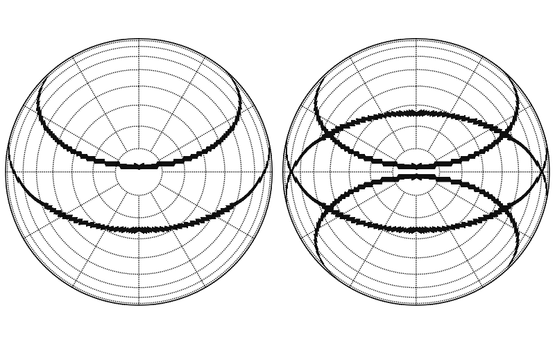
Figure 1.— The building up of source tracks and crossing points. Left: The paths Cygnus A (top) and Virgo A (bottom) take across the beam for the PAPER array in Green Bank. The projection is orthographic with zenith at the center; dotted lines are $10^{\circ}$ and $30^{\circ}$ steps in elevation and azimuth, respectively. Right: The tracks of Cygnus A and Virgo A, and their $180^{\circ}$ rotated images overlaid. There are now 6 crossing points. These are the locations where the beam and source parameters can be solved for independently.

At a crossing point, there are only 3 unknowns, since each source is illuminated by the same primary beam response, $b$. Since two circles on the sky cross twice (if they cross at all), there will be two independent relations that together provide enough information to constrain both the primary beam response at those points and the flux densities of sources passing through them (relative to an absolute flux scale). By using multiple sources, it is possible to build a network of crossing points that covers a large fraction of the primary beam. Furthermore, such a network allows data to be calibrated to one well-measured fiducial calibrator. For observations with the Green Bank deployment of PAPER, source fluxes are related to Cygnus A from Baars et al. (1977).

In the rest of this section, we discuss the algorithmic details of how this approach to primary beam calibration is implemented. These steps are:

1. extracting measurements of perceived source flux densities versus time from observations (§3.1),

2. entering measurements into a gridded sky and finding crossing points (§3.2),

3. solving a least-squares matrix formulation of the problem (§3.3), and, finally,

4. deconvolving the irregularly sampled sky to create a smooth beam (§3.4).

We also discuss prior information that can be included to refine the beam model in §3.5.

3.1. Obtaining Perceived Source Flux Densities

The principal data needed for this approach are measurements of perceived flux density versus time for multiple calibrator sources as they drift through the primary beam. In practice, any method of extracting perceived individual source flux densities (such as image plane analysis) could be used; the beam calibration procedure is agnostic as to the source of these measurements. In this work, we use delay/delay-rate (DDR) filters to extract estimates of individual source flux densities as a function of time and frequency. The frequency information can be used to perform a frequency-dependent beam calibration if the SNR in the observations is high enough. These filters work in delay/delay-rate space (the Fourier dual of frequency/time space) to isolate flux density per baseline from a specific geometric area on the sky; for a full description of the technique, the reader is referred to Parsons & Backer (2009).

The first step of our pipeline to produce perceived flux density estimates is to filter the Sun from each baseline individually in DDR space. This is done to ensure that little to no signal from the Sun, which is a partially-resolved and time-variable source, remains in the data. (In principle, data from different observing runs separated by several months could provide complete sky coverage while avoiding daytime data altogether. We chose to use data from only one 24 hour period to minimize the effect of any long timescale instabilities in the system). A Markov-Chain Monte Carlo (MCMC) method for extracting accurate time- and frequency-dependent source models via self-calibration using DDR-based estimators is then used to model the 4 brightest sources remaining: Cygnus A, Cassiopeia A, Virgo A, and the Crab Nebula (Taurus A). The MCMC aspect of this algorithm iterates on a simultaneous model of all sources being fit for to minimize sidelobe cross-terms between sources. After removing the models of Cygnus A, Cassiopeia A, Virgo A and Taurus A from the data, a second pass of the MCMC DDR self-calibration algorithm extracts models of the remaining 22 sources listed in Table LABEL:srctable.

3.2. Gridding the Measurements

We can increase the signal-to-noise at a crossing point by combining all measurements within a region over which the primary beam response can be assumed to be constant. To define these regions, we grid the sky. In this work, the beam model is constructed on an HEALPix map (Górski et al., 2005) with pixels $\approx 0.9^{\circ}$ on a side. The choice of grid pixel size is somewhat arbitrary. Using a larger pixel size broadens the beam coverage of each source track, creating more crossing points and helping to constrain the overall beam shape. However, when the pixels are too large, each pixel includes data from sources with larger separations on the sky. Since the principal tenet of this approach is that each source within a crossing point sees the same primary beam response, excessively large pixels can violate this assumption, resulting in an inaccurate beam model. For PAPER data, a HEALPix grid with $0.9^{\circ}$ pixels is found to be a good balance between these competing factors, as will be explained in §4.1. For other experiments with narrower, more rapidly evolving primary beams, smaller pixels may be necessary.

To introduce our measurements of perceived flux density into the grid, we first recast Equation 1 into a discrete form:

$$M_{i}=b_{i}f_{k},$$ (2)

where $M_{i}$ and $b_{i}$ are the respective perceived source flux densities and primary beam responses in the pixel $i$, and $k$ is a source index labelling the inherent source flux density, $f$. To generate a single measurement of a source for each pixel $i$, we use a weighted average of all measurements of that source falling with a single pixel. The weights are purely geometric and come from interpolating the measurement between the four nearest pixels.

3.3. Forming a Least-Squares Problem

Once all the data are gridded, we solve Equation 2 for all crossing pixels simultaneously. To do this, we set up a linearized least-squares problem using logarithms:

$$\log(M_{i})=\log(b_{i})+\log(f_{k}).$$ (3)

Because thermal noise in measurements becomes non-Gaussian in Equation 3, the solution to the logarithmic formulation of the least-squares problem is biased. In §4.1, we investigate the effect of this bias using simulations and find that the accuracy of our results is not limited by this bias, but instead by sidelobes of other sources. Therefore, while Equation 1 can in principle be solved without resorting to logarithms using an iterative least-squares approach, we find that this is not necessary given our other systematics.

Once the logarithms are taken, we can construct a solvable matrix equation, which can be expressed generally as:

$$\mathbf{WM=WAX},$$ (4)

where $\mathbf{W}$ is a column-matrix of weights, $\mathbf{M}$ is a column-matrix of measurements, $\mathbf{A}$ is the matrix-of-condition, describing which measurements are being used to constrain which parameters, and $\mathbf{X}$ is a column matrix containing all the parameters we wish to measure: the beam responses $b$ and the source flux densities $f$. To illustrate the form of this equation, we present the matrix representation of the Cygnus A/Virgo A system shown in Figure 1:

$${\left(\begin{array}[]{c}W_{1}\\ W_{2}\\ W_{3}\\ W_{4}\\ W_{5}\\ W_{6}\\ W_{7}\\ W_{8}\\ W_{9}\\ W_{10}\\ W_{11}\\ W_{12}\end{array}\right)}{\left(\begin{array}[]{c}\log M_{1}\\ \log M_{2}\\ \log M_{3}\\ \log M_{4}\\ \log M_{5}\\ \log M_{6}\\ \log M_{7}\\ \log M_{8}\\ \log M_{9}\\ \log M_{10}\\ \log M_{11}\\ \log M_{12}\end{array}\right)}={\left(\begin{array}[]{c}W_{1}\\ W_{2}\\ W_{3}\\ W_{4}\\ W_{5}\\ W_{6}\\ W_{7}\\ W_{8}\\ W_{9}\\ W_{10}\\ W_{11}\\ W_{12}\end{array}\right)}{\left(\begin{array}[]{cccccc|cc}1&0&0&0&0&0&1&0\\ 1&0&0&0&0&0&0&1\\ 0&1&0&0&0&0&1&0\\ 0&1&0&0&0&0&0&1\\ \hline\cr\ 0&0&1&0&0&0&1&0\\ 0&0&1&0&0&0&0&1\\ 0&0&0&1&0&0&1&0\\ 0&0&0&1&0&0&0&1\\ \hline\cr\ 0&0&0&0&1&0&0&1\\ 0&0&0&0&1&0&0&1\\ 0&0&0&0&0&1&0&1\\ 0&0&0&0&0&1&0&1\end{array}\right)}{\left(\begin{array}[]{c}\log b_{1}\\ \log b_{2}\\ \log b_{3}\\ \log b_{4}\\ \log b_{5}\\ \log b_{6}\\ \log f_{cyg}\\ \log f_{vir}\end{array}\right)}$$ (61)

On the left-hand side of the equation are the two column matrices $\mathbf{W}$ and $\mathbf{M}$. The weights, $W_{i}$, are defined in §3.3.1. $\mathbf{M}$ contains logarithms of the perceived source flux density measurements in each pixel, $M_{i}$. Recall that each $M_{i}$ corresponds to one source.

On the right-hand side, the weighting column matrix $\mathbf{W}$ appears again, followed by the matrix-of-condition $\mathbf{A}$, and then $\mathbf{X}$, a column matrix containing the parameters we wish to solve for: the primary beam response at the 6 crossing points and the flux densities of Virgo and Cygnus. The matrix-of-condition, $\mathbf{A}$, identifies which sources and crossing points are relevant for each equation. We have schematically divided it: to the left of the vertical line are the indices used for selecting a particular crossing point; to the right are those for the sources. The first 4 lines represent the two northern Cygnus/Virgo crossing points, and the next four represent the two southern ones (which are identical copies of the northern ones). Finally, the last 4 lines represent the 2 points where Virgo crosses itself; notice that the Cygnus source column is blank for these 4 rows.

It should be noted that Equations 4 and 61 contains no absolute flux density reference. The simplest way to set this scale is to treat all the recovered flux densities as relative values compared to the flux calibrator (Cygnus A in the case presented here). One can then place all the flux densities onto this absolute scale. An equally valid approach is to append an extra equation with a very high weight, which sets the flux calibrator to its catalog flux value.

3.3.1 Weighting of Measurements in the Least-Squares Formalism

In a least-squares approach, optimal weights are inversely proportional to the variance of each measurement. To calculate the variance of each measurement, we must propagate the uncertainty in the initial perceived flux density measurements through the averaging and logarithm steps. The noise level in each interferometric visibility is roughly constant, and the DDR filters average over a fixed number of visibilities for each perceived flux density estimate, leading to equal variance at each time sample. To produce optimal weights accounting for the many time samples averaged into each beam pixel and the propagation of noise through the logarithm, each logarithmic measurement in Equation 4 should be weighted by:

$$W_{i}=\sqrt{M_{i}^{2}\sum\limits_{j}w_{j}},$$ (62)

where $j$ indexes the time step (which is generally fast enough to produce many measurements inside a pixel), $w_{j}$ is the geometric sub-pixel interpolation weighting of each measurement, and $M_{i}$ is the weighted average of all measurements of a source’s flux density in pixel $i$. Without the square root, these weights would be proportional to the inverse of the variance in each logarithmic measurement; the sum over the geometric weights is the standard reduction of variance for a weighted average, and the factor of $M_{i}^{2}$ comes from propagating variances through the logarithm. The square root appears because a least-squares solver using matrix inversion will add in an additional factor of the weight, leading to the desired inverse-variance weighting. Other solvers using different methods may require different weights.

3.3.2 Solving the Least-Squares Equation for a First-Order Beam Model

The solution of Equation 4, the matrix $\mathbf{A}$, contains two distinct sets of parameters: the beam responses at crossing points and the flux densities of each source (modulo an absolute scale). There is additional information that may be included to improve the beam model beyond that generated by solving for the responses at crossing points. Given the flux-density solutions for each source, each source track now provides constraints on beam pixels that are not crossing points. By dividing each perceived flux density source track by the estimated inherent flux density from the least-squares inversion, we produce a track of primary beam responses, with greater coverage than that provided by crossing points alone. We illustrate the difference in coverage in Figure 2.

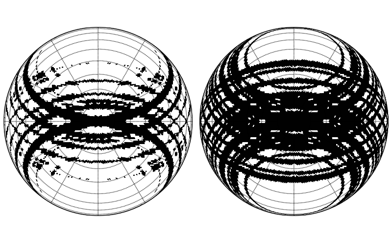
Figure 2.— The sky coverage of crossing points and source tracks. Left: The location of crossing points for the 25 sources listed in Table LABEL:srctable used to calibrate the PAPER primary beam. The projection is orthographic with zenith at the center; dotted lines are $10^{\circ}$ and $30^{\circ}$ steps in elevation and azimuth, respectively. Right: The sky coverage of all 25 source tracks. Although the least-squares inversion solves only for the beam response at crossing points, we can include all source track data using the recovered flux density of each source to create a primary beam estimate along the entire track.

The left hand panel shows the locations of crossing points for the 25 sources used to calibrate the PAPER beam, listed in Table LABEL:srctable. The right hand panel shows the increased beam coverage that comes from including non-crossing point source-track data. To create an initial beam model, we average within each pixel the estimated beam responses from each source, weighting by the estimated flux of that source. Given equal variance in each initial perceived flux density measurement, this choice of weights is weighting by signal to noise.

3.4. Using Deconvolution to Fill in Gaps in the Beam Model

To produce a model of the beam response in any direction, we must fill in the gaps left by limited sky sampling. We use a CLEAN-like (Högbom, 1974) deconvolution algorithm in Fourier space to fill in the holes in the beam. We iteratively fit and remove a fraction of the brightest Fourier component of our beam until the residuals between the model and the data are below a specified threshold. In addition to measured beam responses derived from source tracks, we add the constraint that the beam must go to zero beyond the horizon. In the deconvolution, each pixel is weighted by the estimate of the beam response in that pixel, reflecting that SNR will be highest where the beam response is largest. This beam-response weighting was unnecessary in previous steps, since the least-squares approach solved for each pixel independently. This weighting scheme again represents signal-to-noise weighting, given the equal variance in our initial perceived flux density estimates. The result of the deconvolution is an interpolated primary beam model with complete coverage across the sky.

3.5. Introduction of Prior Knowledge

Up to this point, we have made only two fairly weak assumptions about our beam: that it possesses $180^{\circ}$ rotational symmetry, and that the response is zero below the horizon. However, if we have additional prior knowledge about our beam, we can better constrain the final model. In particular, we can use beam smoothness constraints to identify unphysically small scale features introduced by sidelobes in the source extraction or by incomplete sampling in the deconvolution. We choose to incorporate additional smoothness information by filtering our model in Fourier space to favor large-scale modes.

PAPER dipoles were designed with emphasis on spatial and spectral smoothness in primary beam shape. To smooth the PAPER beam model, we choose a cutoff in Fourier space that corresponds to the scale at which $>99.9\%$ of the power is accounted for in a computed electromagnetic model of the beam. While such a filter is not necessarily generalizable to other antenna elements, we find it necessary to suppress the substantial sidelobes associated with observations from a 12-antenna PAPER array that are discussed below.

4. Application to Simulated Data

To test the robustness of this approach, we apply it to several simulated data sets. The results of these simulations, with and without Gaussian noise, are described below in §4.1. We also simulate raw visibility data to test the effectiveness of source extraction; these simulations are discussed in §4.2. The major difference between these two methods of simulation is that the simulation using raw visibility data allows for imperfect source isolation, leading to contamination of the source tracks by sidelobes of other sources. These sidelobes have a significant effect on the final beam model that is derived.

4.1. Simulations of Perceived Flux Density Tracks

We simulate perceived flux density tracks using several model beams of different shapes, including ones with substantial ellipticity and an $\sim 15^{\circ}$ rotation around zenith. We also input several source catalogs, including a case with $10,000$ Jy sources spaced every degree in declination, and a case using the catalog values and sources listed in Table LABEL:srctable that approximately match the sources extracted from observations. In all combinations of beam models and source catalogs, we recover the input beam and source values with $<5\%$ error. The average error in source flux density is 2.5%. We see no evidence for residual bias, as the distribution of error is consistent with zero mean to within one standard deviation.

We also test the effect of adding various levels of Gaussian noise to a simulation involving a fiducial beam model and the 25 sources listed in Table LABEL:srctable. Only when the noise level exceeds an RMS of 10 Jy in each perceived flux density measurement does the mean error in the solutions exceed 10%. As the noise increases beyond this level, there is a general trend to bias recovered flux densities upward; as mentioned earlier, this bias is introduced by the logarithms in Equation 3. However, the expected corresponding noise level of DDR-extracted perceived flux density measurements from our 12-element PAPER array is $<1$ Jy per sample. At a simulated rms noise level of 1 Jy, the solutions are recovered with a mean error of $<3\%$. This result validates our previous statement that the bias introduced by the logarithms in Equation 3 is not a dominant source of error.

It is also worth noting that these simulations were used to identify $0.9^{\circ}$ as the best HEALPix pixel side for our grid; with too large a pixel size ($1.8^{\circ}$) the model becomes significantly compromised. This results from combining measurements of sources that are subject to significantly different primary beam responses. We choose not to use a smaller pixel size, since it will reduce the fractional sky coverage of our crossing points and increase the computational demand of the algorithm.

4.2. Simulations of Visibilities

We also apply this technique to simulated visibilities in order to test the complete analysis pipeline, including the DDR-based estimation of perceived source flux densities. The visibility simulations are implemented in the AIPY software toolkit. The simulated observations correspond to actual observations made with the 12-element PAPER deployment in Green Bank described in §5. We match the observations in time, antenna position, and bandwidth. We also include the expected level of thermal noise in the simulated visibilities. We simulate “perceived” visibilities by attenuating the flux density of each source by a model primary beam. The DDR filters return estimates of perceived source flux density for the input primary beam.

In these simulations, we only include bright point sources and a uniform-disk model of the Sun. As a result, source extraction is expected to be more accurate in simulation than in real data, since the sources we extract account for $100\%$ of the simulated signal. However, these simulations do provide a useful test of DDR-filter-based source extraction and of the level of contamination from sidelobes.

As might be expected, the estimates of perceived source flux density versus time from simulated visibilities contain structure that is not attributable to the beam. These features are almost all due to sidelobes of other sources; they persist in real data and are reproducible over many days. Figure 3 shows the difference in the source tracks produced for Cassiopeia A by each simulation method (cases 1 and 2 in the figure), as well as the track extracted from the observed data described §5 (case 3).

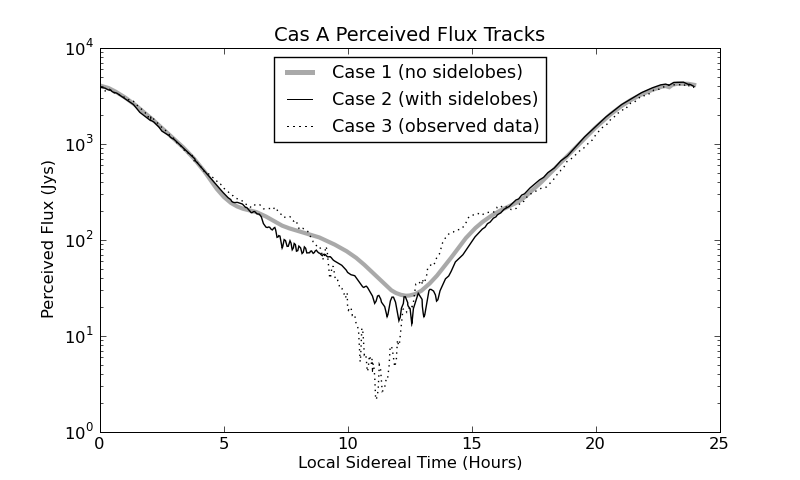
Figure 3.— Three different perceived flux tracks for Cassiopeia A. Case 1 is simply a cut through a model beam multiplied by a catalog flux density value; this is the simplest case and contains no sidelobe contamination. Case 2 uses DDR filters to extract the source track from simulated visibilities; case 3 does the same, but applied to observed data. The simulated visibilities in case 2 demonstrate the features that arise from sidelobes of other sources during the DDR source extraction. However, the simulation employs a simplistic point-source sky and cannot reproduce all sidelobe features seen in the real data.

We find that the DDR filter only extracts a fraction of the flux density from the Crab Nebula. This bias is unique to Crab, and is most likely a result of the proximity of the Sun to Crab in these observations, coupled with the limited number of independent baselines in the 12-antenna array. For this reason, we choose to exclude the Crab from our final analysis.

Performing the least-squares inversion described in §3.3 on the simulated source tracks, we find that the sidelobes introduce errors into estimates of source flux densities. The average error in flux density is 10%, with the largest errors exceeding 20%. The distribution of errors is consistent with zero mean, indicating no strong biasing of the flux densities.

We also find that the resultant primary beam model matches the input beam to within 15% percent. However, the model contains small scale variations, as seen in Figure 4.

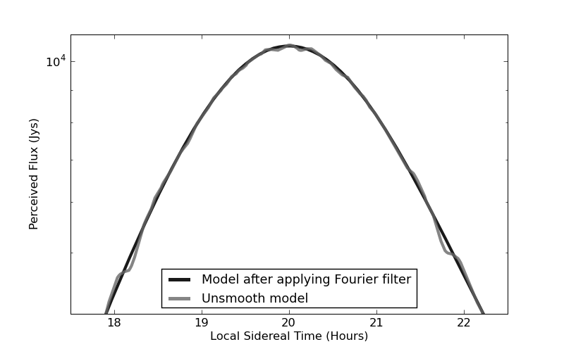
Figure 4.— The effect of the Fourier domain filter. The deconvolution of §3.4 fills in gaps in sky coverage, but leaves small scale structure that is not associated with the primary beam (gray curve). By filtering the solution in the Fourier domain to incorporate prior knowledge of beam smoothness, one can achieve an improved beam model (black curve).

Using prior knowledge of beam smoothness, we can reject these features as unphysical and apply a Fourier-domain filter, as described in §3.5. This filter reduces the effect of sidelobes in the source tracks, as they appear on Fourier scales that are not allowed by smoothness constraints. Even with a relatively weak prior on smoothness (i.e., retaining more Fourier modes than are present in our input model), we substantially reduce the small scale variations in our beam. The effect of the filter on small scale variations is illustrated in Figure 4. The filter also reduces large scale errors in the model, bringing the overall agreement to with 10% of the input beam.

In summary, we find that although interfering sidelobes from other sources compromise our source flux density measurements, our approach recovers the input primary beam model at the 15% level. With the introduction of a Fourier space filter motivated by prior knowledge of the beam smoothness, the output model improves to within 10% of the input. It is also worth noting that the effectiveness of the beam calibration technique presented here will substantially improve with larger arrays, where sidelobe interference will be reduced and source tracks will more closely resemble the ideal case discussed in §4.1.

5. Observed Data

In this section, we describe the application of this technique to 24 continuous hours of data taken with the PAPER array deployed at the NRAO site near Green Bank from July 2 to July 3, 2009. At this time, the array consisted of 12 crossed-dipole elements. Only the north/south linear polarization from each dipole was correlated. The data used in this analysis were observed between 123 to 170 MHz (avoiding RFI) and were split in 420 channels. The array was configured in a ring of 300m radius. The longest baselines are 300m, while the shortest baseline is 10m; the configuration is shown in Figure 5. This configuration gives an effective image plane resolution of $0.4^{\circ}$.

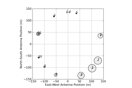
Figure 5.— The 12 element PAPER array in Green Bank. Shaded circles represent vertical height relative to antenna 0; the radius of the circle is 10 times the height in meters. Light gray is up, dark gray is down.

5.1. Data Reduction

In addition to the DDR-filter algorithm described in §3.1, several other pre-processing steps are necessary. Per-antenna phase and amplitude calibration are performed by fringe fitting to Cygnus A and other bright calibrator sources. We also use a bandpass calibration based on the spectrum of Cygnus A. This calibration is assumed to be stable over the full 24 hours. Two further steps in the reduction pipeline were first described in Parsons et al. (2010): gain linearization to mitigate data quantization effects in the correlator, and RFI excision.

New to this work is the use of the cable and balun temperatures to remove time-dependent gains caused by temperature fluctuations. A thirteenth dipole was operated as the “gain-o-meter” described in Parsons et al. (2010). In brief, the “gain-o-meter” is an antenna where the balun is terminated on a matched load, rather than a dipole. The measured noise power from this load tracks gain fluctuations in the system. We record the temperature of several components of our “gain-o-meter” using the system described in Parashare & Bradley (2009). We find a strong correlation between the absolute gain of our system and the temperature of these components; this effect is illustrated in Figure 6.

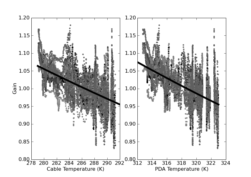
Figure 6.— The effect of ambient temperature on the system gain, derived from observations of Cygnus A near zenith, where beam effects are unimportant. The left-hand side shows the effect of the cable temperature; the right shows pseudo-differential amplifier (PDA)/balun temperature. The solid black line is the best fit to the data. Different shades of gray represent data from different antennas.

We correct for these gain changes by applying a linear correction derived from the measured temperature values. This step is crucial for the success of the beam calibration; without correcting for them, these gain drifts are indistinguishable from an east/west asymmetry in the primary beam. After these steps, we process the data with the DDR-filtering algorithm to produce estimates of perceived flux density versus time for the 25 sources listed in Table LABEL:srctable.

5.2. Results

5.2.1 PAPER Primary Beam Model

The first estimate of the PAPER primary beam derived with this approach is shown in Figure 7.

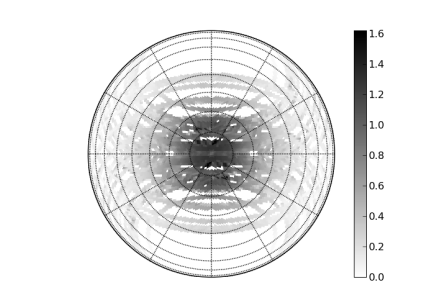
Figure 7.— The initial solution for the PAPER primary beam response along source tracks. Each perceived flux density track is divided by the estimate of that source’s inherent flux density produced by the least-squares inversion. This yields estimates of the primary beam response along each track. With this initial solution, a large fraction of the sky is already covered by the data, although there is a fair bit of variation from point to point. The color scale is linear and normalized to 1.0 at zenith; as in Figure 1, dotted lines are $10^{\circ}$ and $30^{\circ}$ steps in elevation and azimuth, respectively.

This figure is produced by dividing each source track by an estimate of its inherent flux density produced by the least squares inversion. This transforms each track into an estimate of the primary beam response, which are the added together into a HEALPix map. There are significant fluctuations from pixel to pixel that are clearly unphysical, and relate to source sidelobes. There are also significant gaps in beam coverage, even with 25 source tracks.

Figure 8 show the results after deconvolving the sampling pattern from Figure 7.

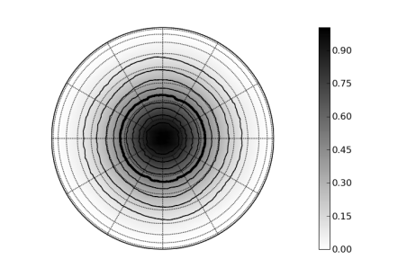
Figure 8.— The deconvolved PAPER beam model. The grayscale colors are linear and show the primary beam response, normalized to 1.0 at zenith. Solid black lines are contours of constant beam response in 10% increments; the thick black line is the half-power point. As in Figure 1, dotted lines are $10^{\circ}$ and $30^{\circ}$ steps in elevation and azimuth, respectively. This model was produced by deconvolving the sampling pattern from Figure 7, interpolating over the gaps in declination where there are no strong calibrator sources.

The beam is now complete across the entire sky, although there is still substantial small-scale structure unrelated to the inherent beam response. We suppress these features in our final model by retaining only the large scale Fourier components, as described in §3.4. This final model is shown in Figure 9.

Figure 9.— The smooth PAPER beam model. As in Figure 8, the grayscale colors are linear and show the primary beam response, normalized to 1.0 at zenith. Solid black lines are contours of constant beam response in 10% increments; the thick black line is the half-power point. Dotted lines are $10^{\circ}$ and $30^{\circ}$ steps in elevation and azimuth, respectively. This smooth model was produced by retaining only the large scale Fourier components from Figure 8. The cutoff in Fourier space was derived from a computed electromagnetic PAPER beam simulation. This Fourier mode selection substantially smooths out variations in the initial solution that are unphysical based on the smoothness of beam response in the simulation.

It is clear that with our deconvolution and choice of Fourier modes, we recover a very smooth, slowly evolving beam pattern, as expected from previous models of the PAPER primary beam.

5.2.2 Source Catalog

The measured flux densities of the calibrator sources, produced by the least-squares inversion, are presented in Table LABEL:srctable. The overall flux scale is normalized to the value of Cygnus A reported in Baars et al. (1977). Error-bars are estimated by measuring the change in flux necessary to increase $\Delta\chi^{2}$ between the model and the measured perceived source flux density tracks by 1.0. As noted in §4.2, these flux densities can be compromised by sidelobes of other sources. However, the results are generally accurate to within $\pm 10\%$.

5.3. Tests of Validity

We perform several tests to investigate the validity of our results. The comparison of our recovered fluxes to their catalog values shows generally good agreement. As argued in Vollmer et al. (2005) and Jacobs et al. (2011), there is considerable difficulty in accurately comparing catalogs, particularly at these frequencies. Differences in interferometer resolution and synthesized beam patterns can lead to non-trivial disagreement in measured source flux densities. Given this fact, and the complicated sidelobes associated with a 12-element array present in our method, we do not find the lack of better agreement with catalog fluxes troubling.

To test the stability of our pipeline, we test a separate observation spanning the following day. The beam model produced by this data matches our first model to within 2.5%, and source flux densities remain consistent to 5%. This test confirms our suspicion that our errors are not dominated by random noise.

6. Conclusions

We have presented a new technique for calibrating the primary beam of a wide-field, drift-scanning antenna element. The key inputs to the method are measurements of perceived flux density of individual sources versus time as they drift through the beam. In this paper, we use delay/delay-rate filters (Parsons & Backer, 2009) as estimators in a self-calibration loop to extract such measurements from raw interferometric data. However, the remainder of our method is agnostic to how these tracks are derived. The only assumption necessary to make this an over-constrained and solveable problem is $180^{\circ}$ rotational symmetry in the beam. With this assumption, we create “crossing points” where there is enough information for a least-squares inversion to solve for both the inherent flux density of each source and the response of primary beam at the crossing points.

We test this approach using simulated tracks of perceived source flux density across the sky and simulated visibilities. Using the source tracks, the least-squares inversion reliably recovers the primary beam values and source flux densities in the presence of noise 10 times that present in a 12-element PAPER array. The simulated visibilities demonstrate that sidelobes of other bright sources are the source of the dominant errors in source extraction when only 12 antennas are used. The presence of these features in the perceived source flux densities limits the accuracy of estimates of inherent source flux densities. However, in simulation, we are able to recover a primary beam model accurate to within 15% percent and source flux densities with an average error of 10%. Using prior information regarding beam smoothness, we improve our model to better than 10% accuracy.

While these caveats about the effectiveness of the least-squares technique in the presence of sidelobes may seem worrisome, it bears repeating that these are issues with data quality and not with the technique itself. For example, data from a 32-element PAPER array has shown that DDR filters can extract the sources used in this analysis with little systematic biases. (We do not use this data here do the lack of a temperature record for gain stabilization and the presence of a particularly active Sun when the array was operating.) Therefore, it seems that this technique has significant potential for precise beam calibration on larger arrays.

Another future goal for this technique is to calibrate the frequency-dependence of the beam. Here, we have used our entire bandwidth to improve signal-to-noise in source extractions. For a larger array with higher SNR and lower sidelobes, our perceived source flux density measurements can be cut into sub-bands to look at the beam as a function of frequency.

Finally, it is possible to forgo the assumption of $180^{\circ}$ rotational symmetry altogether and allow for possible north/south variation in the beam. An experiment in which the dipoles are physically rotated on a daily basis can be used to create the same kind of crossing points, since one has changed the section of the beam each source crosses through. Work is progressing on such an experiment using the PAPER array.

7. Acknowledgements

The PAPER project is supported through the NSF-AST program (award #0804508), and by significant efforts by staff at NRAO’s Green Bank and Charlottesville sites. PAPER acknowledges the significant correlator development efforts of Jason R. Manley. We also thank our reviewer for their helpful comments. ARP acknowledges support from the NSF Astronomy and Astrophysics Postdoctoral Fellowship under award AST-0901961.

[caption=Measured flux densities for all the sources used in this work. Catalog values come from the 3C catalog (Edge et al., 1959) at 159 MHz unless otherwise noted. Errors are estimated by measuring the change in flux required to increase $\Delta\chi^{2}$ between the model and measured perceived flux density source tracks by 1.0., width=label=srctable]c—c——c—c—c[a]3CRR (Laing et al., 1983) at 178 MHz. [b]Culgoora (Slee, 1995) at 160 MHz. [c]PSA32 (Jacobs et al., 2011). Measurements made by PAPER. [d]Extended (35x27 arcmin) supernova remnant (W44). [e]Flux density calibrator, using values from Baars et al. (1977). [f]Extrapolated using the formula in Baars et al. (1977). This is probably a substantial underestimate of the flux density, as suggested by Helmboldt & Kassim (2009). RA & Dec Measured Flux Density (Jy) Catalog Flux Density (Jy) Name
1:08:54.37 +13:19:28.8 $78.1^{+14.7}_{-24.4}$ 58, 49[a] 3C 33
1:36:19.69 +20:58:54.8 $47.3^{+12.3}_{-37.3}$ 27 3C 47
1:37:22.97 +33:09:10.4 $60.0^{+10.2}_{-13.7}$ 50 3C 48
1:57:25.31 +28:53:10.6 $36.2^{+9.8}_{-23.6}$ 7.5, 16[b], 23[c] 3C 55
3:19:41.25 +41:30:38.7 $81.7^{+12.0}_{-16.5}$ 50 3C 84
4:18:02.81 +38:00:58.6 $75.9^{12.2}_{-14.0}$ 60 3C 111
4:37:01.87 +29:44:30.8 $205.3^{+26.9}_{-32.1}$ 204 3C 123
5:04:48.28 +38:06:39.8 $100.3^{+17.0}_{-20.2}$ 85 3C 134
5:42:50.23 +49:53:49.1 $56.5^{+9.7}_{-11.5}$ 63 3C 147
8:13:17.32 +48:14:20.5 $66.3^{+9.5}_{-9.9}$ 66 3C 196
9:21:18.65 +45:41:07.2 $48.5^{+7.5}_{-9.0}$ 42 3C 219
10:01:31.41 +28:48:04.0 $40.3^{+8.7}_{-15.6}$ 30 3C 234
11:14:38.91 +40:37:12.7 $34.5^{+7.0}_{-19.9}$ 21.5 3C 254
12:30:49.40 +12:23:28.0 $1108.9^{+29.6}_{-28.1}$ 1100 Vir A
14:11:21.08 +52:07:34.8 $64.4^{+6.4}_{-6.7}$ 74 3C 295
15:04:55.31 +26:01:38.9 $73.5^{+7.4}_{-9.0}$ 72 3C 310
16:28:35.62 +39:32:51.3 $60.5^{+7.2}_{-12.4}$ 49 3C 338
16:51:05.63 +5:00:17.4 $461.7^{+78.6}_{-112.7}$ 325[a], 378[b], 373[c] Her A
17:20:37.50 -0:58:11.6 $228.8^{+61.7}_{-147.5}$ 180, 236[a], 276[b], 215[c] 3C 353
18:56:36.10 +1:20:34.8 $251.3^{+60.0}_{-135.8}$ 680 3C 392[d]
19:59:28.30 +40:44:02.0 $10622.9^{+126.0}_{-128.9}$ 10623 Cyg A[e]
20:19:55.31 +29:44:30.8 $62.2^{+16.4}_{-28.0}$ 36 3C 410
21:55:53.91 +37:55:17.9 $51.9^{+11.5}_{-16.2}$ 43 3C 438
22:45:49.22 +39:38:39.8 $71.3^{+12.4}_{-19.3}$ 50 3C 452
23:23:27.94 +58:48:42.4 $9198.1^{+203.4}_{-186.9}$ 6230[f] Cas A

References

- Baars et al. (1977) Baars, J. W. M., Genzel, R., Pauliny-Toth, I. I. K., & Witzel, A. 1977, A&A, 61, 99
- Bowman et al. (2008) Bowman, J. D., Rogers, A. E. E., & Hewitt, J. N. 2008, ApJ, 676, 1
- Edge et al. (1959) Edge, D. O., Shakeshaft, J. R., McAdam, W. B., Baldwin, J. E., & Archer, S. 1959, MmRAS, 68, 37
- Ellingson et al. (2009) Ellingson, S. W., Clarke, T. E., Cohen, A., Craig, J., Kassim, N. E., Pihlstrom, Y., Rickard, L. J., & Taylor, G. B. 2009, IEEE Proceedings, 97, 1421
- Furlanetto et al. (2006) Furlanetto, S. R., Oh, S. P., & Briggs, F. H. 2006, Phys. Rep., 433, 181
- Górski et al. (2005) Górski, K. M., Hivon, E., Banday, A. J., Wandelt, B. D., Hansen, F. K., Reinecke, M., & Bartelmann, M. 2005, ApJ, 622, 759
- Helmboldt & Kassim (2009) Helmboldt, J. F., & Kassim, N. E. 2009, AJ, 138, 838
- Högbom (1974) Högbom, J. A. 1974, A&AS, 15, 417
- Jacobs et al. (2011) Jacobs, D. C., et al. 2011, ApJ, 734, L34+
- Laing et al. (1983) Laing, R. A., Riley, J. M., & Longair, M. S. 1983, MNRAS, 204, 151
- Lonsdale et al. (2009) Lonsdale, C. J., et al. 2009, IEEE Proceedings, 97, 1497
- Paciga et al. (2011) Paciga, G., et al. 2011, MNRAS, 413, 1174
- Parashare & Bradley (2009) Parashare, C. R., & Bradley, R. F. 2009, in 2009 USNC/URSI Annual Meeting
- Parsons & Backer (2009) Parsons, A. R., & Backer, D. C. 2009, AJ, 138, 219
- Parsons et al. (2010) Parsons, A. R., et al. 2010, AJ, 139, 1468
- Peterson et al. (2006) Peterson, J. B., Bandura, K., & Pen, U. L. 2006, ArXiv Astrophysics e-prints
- Röttgering (2003) Röttgering, H. 2003, New Astronomy Reviews, 47, 405
- Santos et al. (2005) Santos, M. G., Cooray, A., & Knox, L. 2005, ApJ, 625, 575
- Seo et al. (2010) Seo, H.-J., Dodelson, S., Marriner, J., Mcginnis, D., Stebbins, A., Stoughton, C., & Vallinotto, A. 2010, ApJ, 721, 164
- Slee (1995) Slee, O. B. 1995, Australian Journal of Physics, 48, 143
- Swarup et al. (1991) Swarup, G., Ananthakrishnan, S., Kapahi, V. K., Rao, A. P., Subrahmanya, C. R., & Kulkarni, V. K. 1991, CURRENT SCIENCE V.60, NO.2/JAN25, P. 95, 1991, 60, 95
- Vollmer et al. (2005) Vollmer, B., Davoust, E., Dubois, P., Genova, F., Ochsenbein, F., & van Driel, W. 2005, A&A, 436, 757