Semileptonic decays of the Higgs boson at the Tevatron
Abstract
We examine the prospects for extending the Tevatron reach for a Standard Model Higgs boson by including the semileptonic Higgs boson decays for , and for , where is a hadronic jet. We employ a realistic simulation of the signal and backgrounds using the SHERPA Monte Carlo event generator. We find kinematic selections that enhance the signal over the dominant +jets background. The resulting sensitivity could be an important addition to ongoing searches, especially in the mass range . The techniques described can be extended to Higgs boson searches at the Large Hadron Collider.
FERMILAB-PUB-11-499-T
CERN-PH-TH-2011-237
1 Introduction
The Standard Model (SM) predicts a neutral Higgs boson particle whose couplings to other particles are proportional to the particle masses, and that couples to photons and gluons via one-loop-generated effective couplings. While the Higgs boson mass is not predicted, the relation between the Higgs boson mass and its width is fixed from the predicted couplings. Virtual Higgs boson contributions to electroweak precision observables have been computed, and precision data favor at 95% confidence level [1]. Searches at the CERN Large Hadron Collider have produced 95% confidence level exclusion of a SM Higgs boson for a broad mass range above 145 GeV [2, 3].
Because of small signal cross sections and large backgrounds, the search for the Higgs boson in experiments at the Fermilab Tevatron is very challenging, even with the large final datasets approaching per experiment. Nevertheless both the CDF and DØ experiments have achieved steady improvements in their sensitivities in multiple channels to a SM Higgs boson, and their individual results already exclude a SM Higgs boson in the mass range – and –, respectively, at 95% confidence level [4, 5, 6]. This exclusion relies mainly on sensitivity to the dilepton final-state decay chain analyzed in Refs. [7, 8, 9] : where or .
Here we examine the prospects for extending the Tevatron reach by including a search for the semileptonic Higgs boson decays for , and for , where is a hadronic jet. This process was first considered as a potential Higgs boson discovery channel for the SSC [10, 11, 12, 13], emphasizing the case of a very heavy Higgs boson, where the “golden mode” becomes limited by its small branching fraction and the broad Higgs boson width. Similar to the golden mode, the semileptonic modes are (almost) fully reconstructible: assuming that the leptonic is close to on-shell, the mass constraint gives an estimate of the unmeasured longitudinal momentum of the neutrino, up to a two-fold ambiguity [13]. For the overall decay rate is 6 times larger than any other SM Higgs boson decay mode with a triggerable lepton. Including these semileptonic channels thus offers the distinct possibility of significantly extending the Tevatron reach over a rather broad mass range.
This channel suffers from large backgrounds from SM processes with a leptonically decaying boson. These include diboson production, top quark production, and direct inclusive +2-jet production. There is also a purely QCD background that is difficult to estimate absent a dedicated analysis with data. The dominant background is inclusive +2-jets; from this background alone we have estimated a signal to background ratio () of , after nominal preselections. Though worrisome, this is not smaller than the analogous for the and modes after preselection in the successful Tevatron analyses of [14, 15, 16, 17, 18, 19].
A drastic reduction in both the +2-jet and diboson backgrounds to semileptonic Higgs boson decay can be achieved by forward jet tagging, i.e. by restricting to Higgs boson production from vector boson fusion (VBF) [10, 20]; it is estimated that the additional requirement of forward jet tagging then gives a factor of 100 reduction in these backgrounds. However the reduction in the Higgs signal, versus inclusive Higgs boson production, is also severe: a factor of 10 at the Tevatron [21]. Looking at the similar trade-off for the dilepton channel, a Tevatron study [22] concluded that the overall sensitivity does not improve by restricting to VBF Higgs boson versus inclusive Higgs boson production. We do not know of any comparable analysis for the semileptonic channel.
For inclusive Higgs boson production at the Tevatron, the semileptonic channels were first studied by Han and Zhang [7, 8]. In a parton-level study with some jet smearing they found that, after basic acceptance cuts together with a veto on extra energetic jets designed to suppress the background, the remaining background is completely dominated by +2-jets. Han and Zhang then made additional kinematic selections that enhance the signal to background ratio . For they thus obtained a significance estimate of for of integrated Tevatron luminosity. The fully differential Higgs boson decay width for this process was exhibited by Dobrescu and Lykken [23], who analyzed the basic kinematics and angular distributions that characterize the Higgs signal.
We improve on these studies by including realistic parton showering (since parton-level jet smearing is inadequate), an NLO-rate improved treatment of the Higgs boson decays (including off-shell effects), and a resummed NNLO estimate of the production cross section. The first two improvements are incorporated by the use of SHERPA [24, 25], a general purpose showering Monte Carlo program, for simulation of both the signal and the inclusive +2-jets background. The NNLO signal cross section is modeled by a -factor.
Our purpose is to study these semileptonic Higgs boson decay channels in a systematic way, but not to mimic a fully-optimized experimental analysis. The DØ experiment has already reported on a semileptonic Higgs boson search using of Tevatron data [26, 27]; this analysis uses multivariate decision trees to enhance the significance of the result. Here we will limit ourselves to simple cuts, in order to make the features of the analysis and the underlying physics more explicit. We study the Higgs signal in the mass range – to reasonably cover the below, near and above threshold regions for Higgs boson decay to two on-shell bosons.
In Section 2 we outline the strategy and define several useful observables. In Section 3 we discuss inclusive Higgs boson production from the dominant gluon–gluon fusion mechanism, and implement a -factor correction to the SHERPA result. In Section 4 we introduce basic preselections and develop cuts implemented in SHERPA to enhance ; this section also contains our main results. We conclude in Section 5 with caveats about the limitations of our analysis and suggestions for further improvements. Cross-checks and additional material are presented in the appendices.
2 Strategy and key observables
We are interested in the Higgs boson decay
| (1) |
and the similar decay with a muon in the final state. In general we take both bosons off shell. We will write as where is the jet with higher transverse momentum (), and noting that physical observables will be symmetric under . We use a baseline selection adopted from the DØ analysis to define reconstructed jets and leptons and impose realistic acceptance cuts. We will assume that events with more than one reconstructed lepton are vetoed, but we want to allow the possibility of extra jets in order to increase signal efficiency. When more than two jets are present there is a combinatorial problem; we will define a Higgs boson candidate selection algorithm that assigns which two jets to use in the Higgs boson reconstruction; these jets may or may not correspond to the two leading jets in the event. It is important to note that this algorithm is chosen so as to optimize the signal sensitivity after the full selection, which is not equivalent to maximizing the number of correctly reconstructed signal events.
When the leptonically decaying boson is (close to) on-shell, these decays are fully reconstructible up to a two-fold ambiguity in the neutrino momentum without making any assumption about the Higgs boson mass. Here we are assuming that the transverse momentum of the neutrino is well estimated given a measurement of the missing transverse energy (MET), as has been demonstrated by both Tevatron experiments in the determination of the boson mass.
The semileptonic channel’s advantage of being, in principle, completely reconstructible offers a great way to separate signal from backgrounds. However, when the leptonically decaying boson is far off shell, a straightforward full reconstruction is not possible. There are then three generic possibilities for how to proceed:
- •
Use only transverse observables.
- •
Perform an approximate event-by-event reconstruction using an estimate of the off-shell boson mass.
- •
Perform an approximate event-by-event reconstruction using a (hypothesized) Higgs boson mass constraint.
Since it is not clear a priori which of these approaches maximizes the Higgs boson sensitivity, we will pursue all three and compare the results.
Given an event-by-event approximate combinatorial full reconstruction of the putative decaying Higgs boson, one can approximately reproduce the kinematics in the Higgs boson rest frame. The true Higgs boson rest frame is given by a longitudinal boost from the lab frame together with a transverse boost defined by the transverse momentum of the Higgs boson. An explicit representation for the four-momenta in the Higgs boson rest frame is given by:
| (2) |
where we have chosen the dijet plane to coincide to the – plane, and have chosen the positive -axis to be the direction of the leptonically decaying boson. The boost factors of the two bosons relative to the Higgs boson rest frame are given by
| (3) |
and we note the identities
| (4) |
Note that is the angle between jet and the direction of the hadronic boson, as seen in the rest frame, while is the angle between the charged lepton and the direction of the leptonic boson as seen in the rest frame. The azimuthal angle is the angle between the dilepton and dijet planes. Defining
| (5) |
we can calculate the angle between the two jets as seen in the Higgs boson rest frame:
| (6) |
Signal events have a minimum opening angle between the jets as seen in the Higgs boson rest frame:
| (7) |
In the approximate reconstructions that we will employ in our analysis, the Higgs boson mass is approximated by a 4-object invariant mass . The transverse momentum of the Higgs boson is approximated by the 4-object transverse momentum . The dijet boost defined in the Higgs boson rest frame is approximated by , which is the dijet boost defined in the 4-object rest frame, in which we can compute this boost factor via . This is equivalent to using Eqs. (2) where one inserts for each invariant mass its reconstructed counterpart.
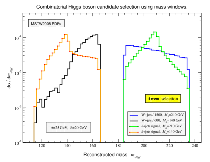
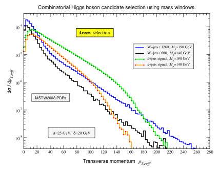
All three of these observables discriminate between Higgs signal and backgrounds. As seen in Figure 1 (top left), for signal events peaks strongly near the true Higgs boson mass, with a width determined primarily by parton shower effects. Thus a simple mass window selection significantly enhances the signal, and since we are interested in Higgs boson exclusion there is no “look-elsewhere” effect associated with imposing mass windows [28]. Note that the backgrounds are not necessarily flat in the mass windows: as seen in Figure 1 the dominant +jets background is rather flat in the high mass window, but is steeply rising in the lower mass window because of the underlying kinematics. In Figure 1 (top right) one sees that the 4-object transverse momentum has a harder spectrum for Higgs signal events than for the +jets backgrounds, independent of the Higgs boson mass.
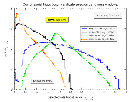
The reconstructed dijet boost has qualitatively different behaviour depending on the underlying Higgs boson mass. When the Higgs boson mass is close to , the distribution of the dijet boost for signal events is strongly peaked near one compared to the distribution for +jets, as seen in Figure 1 (lower left). For larger Higgs boson masses the signal distribution of the dijet boost is instead rather strongly peaked around the value , as expected from Eq. (2).
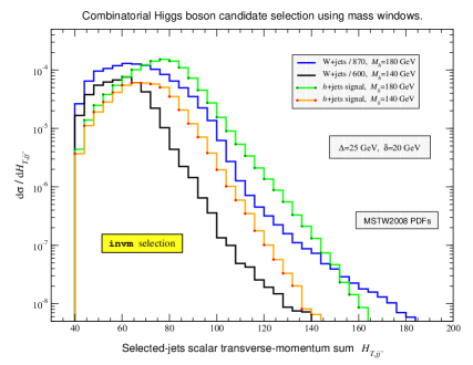
Other physical observables of interest for signal versus background discrimination are defined directly in the lab frame. This includes the 4-object pseudo-rapidity , the pseudo-rapidity difference of the two jets, , and the scalar sum of the two selected jet transverse momenta . As seen in Figure 1 (lower right), the distribution of for signal events is harder than for the +jets background, independent of the Higgs boson mass. From the distributions shown in Figure 12 one sees that the dijet pseudo-rapidity difference has a maximum at zero for signal events (which tend to be confined to the central region), but peaks at a larger value for the +jets background. Similarly from Figure 13 one notes that the 4-object pseudo-rapidity distribution is more central for signal than for the +jets background.
We will also employ various transverse masses, both as signal discriminators and as inputs to the algorithms for the approximate reconstruction of the Higgs boson candidates. One class of observables is solely constructed out of transverse degrees of freedom, ; we define these observables as
| (8) |
where, for the purposes of this study, the labels refer to two, three, or four final-state physics objects (charged lepton, MET, and the two selected jets). We also investigate how our results change when we adopt a slightly different definition that includes the full information from the invariant mass of the visible subset:
| (9) |
where . Here, we have separated the event into a “visible” () and “invisible” () part. The transverse masses are all approximately bounded from above by a kinematic edge; this gives us another handle when fully reconstructing the event. Schematically, we have
| (10) |
where just indicates that in the presence of multiple invisible objects the subsystem enters as a whole when computing Eq. (8). In the 2-particle case, the two transverse-mass definitions coincide provided the single objects are massless.
Given the above arsenal of kinematic discriminators and approximate reconstruction techniques, our basic strategy will be to find the most promising combinations of selections as a function of the Higgs boson mass. Since we are only performing a cut and count analysis, and are lacking a realistic detector description, there is no point in attempting a complete optimization. Instead we will concentrate on providing a comprehensive look at the physics that distinguishes signal from background.
3 Inclusive cross sections and event generation
We use the multi-purpose Monte Carlo event generator SHERPA [24, 25] to pursue our analysis of semileptonic Higgs boson decays in Higgs boson production via gluon fusion. This way we can easily include all (hard and soft) initial-state radiation and final-state radiation (ISR and FSR) effects and arrive at a fairly realistic description of final states as used for detector simulations. Furthermore, sophisticated cuts can be implemented in a straightforward manner owing to the convenient analysis features that come with the SHERPA package. We also want to make use of SHERPA’s capabilities in providing an enhanced modeling of multi-jet final states with respect to a treatment by parton showers only. Apart from a handful of key processes, the SHERPA Monte Carlo program evaluates cross sections at leading order/tree level utilizing its integrated automated matrix-element generators AMEGIC++ [29] and/or COMIX [30]. However, in a number of studies, SHERPA has been shown to generate predictions that are in sufficient, often good agreement with the shapes of kinematic distributions obtained from measurements as well as higher-order calculations; we will give more details in the respective subsections that follow up. Hence, we wish to identify appropriate constant -factors between the most accurate theory results and the leading-order predictions. We in turn want to apply these -factors to correct SHERPA’s predictions for the inclusion of exact higher-order rate effects. Therefore, we study signal and background fixed-order and resummed cross sections at Tevatron Run II energies for the processes
| (11) |
leading to final states consisting of an isolated lepton, missing transverse energy and at least two jets. The label denotes electrons, , and muons, ; the parton label contains light/massless-quark flavours and gluons. Note that final-state gluons may only occur in background hard processes or through the inclusion of I/FSR effects. For the respective -factors, it is not clear a priori at which level of cuts they are defined most accurately. The most convenient definition should be given in terms of the total inclusive cross sections, while one may define more exclusive -factors, if the higher-order tools allow for the specification of the desired cuts. We do not expect a strong dependence on the exact -factor definition provided the shapes are comparable. These issues are examined in more detail below with the goal of determining reasonable signal and background -factors that can be used to rescale the respective leading-order cross sections of the SHERPA predictions, which we take to pursue our signal versus background studies.
3.1 Standard Model Higgs boson production and decay
The signal processes for the final states of interest are summarized by
| (12) |
where the Higgs particles are produced through gluon–gluon fusion and decay into boson pairs that split further into the desired semileptonic final states. There are other Higgs boson production mechanisms that can contribute. In particular, the associated production with the additional vector boson decaying hadronically and the production via vector-boson fusion (VBF) ought to be mentioned in this context. For all production channels, up-to-date theory predictions for the total inclusive cross sections of these events are needed to arrive at reliable acceptance estimates for various Higgs boson masses. Refs. [4, 31, 32] give the most recent overview of the theory calculations and results that are used as input for the ongoing Tevatron (and LHC) SM Higgs boson searches. For the Higgs boson masses we are interested in, it is appropriate to separate the Higgs boson production from its subsequent decays and multiply the production rates by the respective branching fractions, which we obtain from Hdecay [33, 34, 35, 36] for and the Particle Data Group (PDG) listings [37] for the subsequent decays of the bosons.
For our main production channel, the Standard Model Higgs boson production via gluon fusion, we want to use the most precise theoretical predictions that have become available over the last few years, for a great review, we refer to Ref. [32]. Using an effective theory approach, this production channel is known at NNLO including electroweak and mixed QCD–electroweak contributions [38, 39, 40, 41]. For a wide range of Higgs boson masses, these NNLO cross sections have been shown to reproduce the latest results obtained from soft-gluon resummation up to NNLL accuracy, cf. Refs. [42, 43, 44]. To mimic the resummation effects, the optimal scale choice at NNLO is found to be , while for the NNLL calculation one employs common scales of . Both higher-order calculations take the most recent parametrization of PDFs at next-to-next-to-leading order into account where the corresponding PDF sets have been provided by the MSTW group in 2008 [45]. The Tevatron Higgs boson searches use these higher-order cross section predictions to report their combined CDF and DØ upper limits on Standard Model Higgs boson production in the decay mode [14, 15, 16, 4, 46, 17, 18, 19]. Hence, it makes sense to input the same theory cross sections in our studies to guarantee a reasonable level of compatibility between our work and the experimental searches. However, one should keep in mind that different viewpoints exist concerning the determination of the best cross section numbers. For example, in Ref. [47] the authors argue that the 10–15% enhancement seen in the inclusive rates is unlikely to survive the cuts applied in the Tevatron analyses and, therefore, should not be included in the calculation of the limits [48, 49]. On the contrary, the renormalization-group improved resummed NNLO cross sections discussed by Ahrens, Becher, Neubert and Yang in Refs. [50, 51, 52] would yield a further 5–6% increase of the NNLL rates. This is because in their approach Ahrens et al. do not only resum threshold logarithms from soft-gluon emission but also -enhanced terms, which arise in the analytic continuation of the gluon form factor to timelike momentum transfer.
| 2.88 | 3.79 | ||||||||||
| 2.88 | 3.71 | ||||||||||
| 2.87 | 3.69 | ||||||||||
| 2.87 | 3.68 | ||||||||||
| 2.88 | 3.69 | ||||||||||
| 2.82 | 3.60 | ||||||||||
| 2.75 | 3.51 | ||||||||||
| 2.72 | 3.46 | ||||||||||
| 2.67 | 3.39 | ||||||||||
| 2.63 | 3.33 | ||||||||||
| 2.60 | 3.28 | ||||||||||
| 2.58 | 3.25 |
For various Higgs boson masses, Table 1 summarizes the signal cross sections that are of relevance for our studies. Separated from the other entries, the left and right parts of the table show parameters, which we use as input to our analysis. We have used the NNLO inclusive cross sections, , given in the 5th column and multiplied them with the branching ratios listed in the column to the right of it, which we have computed with Hdecay version 3.51.111To obtain the values in Table 1, the NNLO MSTW fit result for the strong coupling, , has been employed, the running of quark masses at NNLO has been enabled and the top and bottom quark masses have been set to and , respectively. The Higgs boson widths shown in the 2nd column are also taken from the Hdecay calculation; they slightly differ from the older values given in [21]. To arrive at the higher-order prediction of our signal cross sections depicted in the 8th column, , we furthermore have accounted for the decays described by the branching ratios for one light lepton species, , and for jets, , and a combinatorial factor of 2 reflecting that either of the bosons may decay leptonically. The NNLO cross sections used here [55] are updated values with respect to the ones published in [38]. The difference can be traced back to the addition of the electroweak real-radiation corrections as encoded in Ref. [39] and the change to top masses of . In the 3rd and 4th columns we respectively also give the cross sections and branching fractions as used by the Tevatron experimentalists in their ongoing searches [4]. These values are in good agreement with the respective numbers used in our study. The other signal cross sections listed in the rightmost part of Table 1 are the LO rates obtained from SHERPA, where the one labelled refers to the use of CTEQ6.6 PDFs [56]. We will discuss these LO results and the corresponding -factors in Section 3.3.1. In the 7th column we show an upper estimate for the signal cross sections if one were to include the contributions from the , and VBF production channels. Over the considered Higgs boson mass range the extra processes would enhance the signal rates resulting from gluon–gluon fusion by about 22–23%. We have determined these estimates by adding to the rates the theory predictions for , and as presented in the July 2010 CDF and DØ Higgs boson searches combination paper [46] (for updated values, cf. [4]) including all necessary branching fractions to arrive at the final states.222For all production channels, we consider the Higgs boson decay as specified in (12), since our selection and reconstruction procedures are tailored to this decay mode, see Section 4. In our analysis we deal with , MET and multiple jets (from the decays as well as I/FSR), thus, the presence of additional jets stemming from other hard decays or VBF does not alter our analysis procedures considerably, in other words the Higgs boson reconstruction and selection procedures are designed in a robust way with respect to additional jet activity. The dominant Higgs strahlung contributions to the semileptonic final states arise from the hadronic decays of the associated vector bosons, where we have used the PDG values and . All other combinations are suppressed by about an order of magnitude. Also, we do not consider more than one lepton, i.e. we implicitly assume an exclusive one-lepton cut. We also neglect the cases where the boson decays invisibly and the associated boson splits up leptonically while . These modes will fail our boson reconstruction. The additional 20% increase resulting from these considerations should be born in mind when acceptances and significances are evaluated in a signal versus background study. For the purpose of the analysis we are pursuing here, we however want to be on the conservative side and solely concentrate on the gluon–gluon fusion events.
3.2 Relevant background processes
Processes that give rise to major background contributions are +jets and multi-jet production, where the latter comes into play because of jets faking isolated leptons and/or MET. The muon channel suffers less from jet fakes reducing the multi-jet background by a factor of 5 with respect to the electron channel. The +jets background can also contribute in cases where one lepton goes missing or a jet mimics a lepton while the decays invisibly. Minor contributions stem from and production. A first DØ search in the semileptonic Higgs boson decay channel shows how these backgrounds compare to each other after basic selection cuts, see Ref. [26]. The largest fraction of 83% occurs from +jets, followed by multi-jets, and contributing with 12%, 3% and 2% to the overall background. The +jets contribution is totally dominated by +jets production; the +jets background, where one of the leptons is missed, is small and makes up less than 1% of the total background.
To gain a better understanding of the backgrounds, we will have a closer look at the major contributor +jets. The multi-jet background cannot be simulated straightforwardly, since it requires detailed knowledge of the experiments and measured fake rates etc. Regarding the minor background contributors, we will study the as well as the – or, more exactly, electroweak – background. Even though they enter at a rather low level after the basic selection compared to +jets, it is necessary to cross-check what number of events remain after more selective cuts have been applied, as will be discussed in Section 4.
Another background contribution that has been discussed is gluon-initiated vector boson pair production [57, 58, 59]. This (quark-loop-induced) process occurs at , the same order as the signal. This background formally arises at NNLO, but under realistic experimental cuts this production channel has been shown to significantly increase e.g. the background at the LHC. At the Tevatron the gluon densities are small, so the impact of is expected to be negligible. This expectation was confirmed in Ref. [60] (a 4‰ effect with respect to the NLO cross section for this decay channel). A more important effect also recently pointed out by Campbell et al. in Ref. [60] is the interference between and , which can result in corrections to the Higgs boson signal cross section. However, interference effects are considerably reduced by requiring the transverse mass of the leptons plus MET system to be smaller than . This type of transverse cut is frequently used in our analyses, so we can safely neglect interference effects in our study.
3.2.1 boson plus jets background
For our first study of +jets production, we explore the dependence of inclusive +jet cross sections on the number of jets and the variation of the common scale used to specify the factorization and renormalization scales, and , respectively. This information will help us identify an optimal definition of the +jets -factor, which we take to improve the rates of the SHERPA predictions. We calculate inclusive +-jet cross sections with MCFM version 5.8 to obtain results that are accurate at NLO in the strong-coupling constant [61, 62, 63]. We also run MCFM at LO to determine explicit NLO-to-LO theoretical -factors.333We only consider bosons decaying into pairs; the charge conjugated process will just double the cross section owing to the initial states at the Tevatron. We employ the LO and NLO MSTW2008 PDFs [45] with and , respectively, and impose cuts according to the parameters given in Section 4.1. Note that we do not account for the so-called triangle cut relating the transverse mass of the boson and the missing energy. Other parameters, such as the electroweak input values of the Standard Model, have been taken according to the MCFM default settings.
| Inclusive +-jet cross sections in pb. | ||||||||||
| % | % | |||||||||
| LO | ||||||||||
| NLO | ||||||||||
| 1.37 | 1.33 | 1.31 | 1.34 | 1.30 | 1.29 | |||||
| LO | ||||||||||
| NLO | ||||||||||
| 1.21 | 1.34 | 1.47 | 1.19 | 1.33 | 1.46 | |||||
| LO | ||||||||||
| NLO | ||||||||||
| 0.89 | 1.16 | 1.41 | 1.10 | 1.28 | 1.52 | |||||
We display our MCFM results in Table 2 for different inclusive jet bins and scale choices . As expected, for each -jet multiplicity, the NLO cross sections are more stable under scale variations with the largest deviations occurring for the more complex +2-jet processes. This is also reflected by the various NLO-to-LO -factors, which vary from about 0.9 to 1.5 for while they are rather constant for ranging from about 1.3 to 1.4 only. For illustrative purposes, we also list the LO and NLO inclusive jet-rate ratios starting with . The +-jet cross sections do not deviate substantially for the two nominal scales chosen, where and , which are determined dynamically for each event. Note that is the scalar sum of the transverse momenta of all particles (partons) in the event, i.e. no jet clustering has taken place. The scales lead to slightly larger rates when compared to those obtained for . This can be traced back to the occurrence of -values that are on average larger in the latter case, since for . For the same reason, the cross section differences become more manifest for . The presence of the second jet gives an extra contribution to per event whereas is less affected. This further enhances the deviation of the and averages.
Given the numbers of Table 2 we can conclude that our knowledge of the +2-jet background is accurate on the level of 20%. A -factor of about should be viewed as the upper limit for correcting LO results; in Section 3.3.2 we will however compare the SHERPA background rates more closely with the results of Table 2 and determine a -factor accordingly.
3.3 Monte Carlo simulation of signal and backgrounds using SHERPA
For reasons outlined at the beginning of Section 3, we use SHERPA version 1.1.3 [24, 25] to generate the +jets signal and background events that are needed to understand the potential of a Standard Model Higgs boson analysis in the lepton + MET + jets channel.444Version 1.1.3 was the last of the previous SHERPA generation; for all our purposes, it models the necessary physics equally well compared to the upgraded versions of the current (1.3.x) generation. Cross-comparisons have confirmed this result. We will employ the results of the previous two subsections to settle the inclusive -factors needed to re-scale SHERPA’s LO predictions and include higher-order rate effects.
The signal and background simulations share a number of common parameters and options that have been set as follows: we simulate all events at the parton-shower level, i.e. we include initial- and final-state QCD radiation, but do not account for hadronization effects and corrections owing to the underlying event, since their impact is considerably smaller with respect to additional QCD radiation arising from the hard processes. The intrinsic transverse motion of quarks and gluons inside the colliding hadrons is however modeled by an intrinsic Gaussian -smearing of and . The electroweak parameters are explicitly given: , , , ; the Higgs boson masses and widths are mutable, taken according to Table 1; the couplings are specified by , and the Higgs field vacuum expectation value and its quartic coupling are given as and , respectively. The CKM matrix is simply parametrized by the identity matrix. The bottom and top quark masses are set to and , respectively, and all other quark masses are zero. To avoid any bias owing to the utilization of different PDFs and in order to develop a consistent picture, signal and background events are generated using the same parton distributions. Our first choice of PDFs is the LO MSTW set MSTW2008lo90cl [45], because its NNLO version has been the preferred PDF set used for the recent calculations of the gluon–gluon fusion Higgs boson production cross sections. The strong coupling is determined by one-loop running with , which is the advertised fit value of the LO MSTW2008 set.
To gain some understanding of PDF effects, we compare our MSTW2008 results against predictions generated with a different PDF set. To fully establish the comparison on the same level as for the MSTW2008 PDFs, signal and background rates have to be predicted from theory using the alternative PDF libraries. We cannot follow this approach here, instead we start out from the same normalization that has been used for the SHERPA predictions calculated with MSTW2008 PDFs. After the application of our cuts we then focus on the differences induced by the alternative PDF set. As our second choice we employ the CTEQ6.6 PDF libraries [56] where the strong coupling is set by and the running of the coupling is again computed at one loop. Notice that SHERPA invokes a 6-flavour running for all strong-coupling evaluations.
3.3.1 Generation of signal events
We simulate signal events with electrons or positrons in the final state according to
| (13) |
The hard process composed as is calculated at LO. The incoming gluons and the quarks arising from the decay undergo further parton showering, which automatically is taken care of by the SHERPA simulation. One ends up with the final states generated at shower level. The hard-process tree-level matrix elements and subsequent parton showers needed for the simulation are provided by the SHERPA modules AMEGIC++ and APACIC++, respectively. For our purpose, it is sufficient to treat the muon final states in exactly the same manner as the electron final states, i.e. the muon decay channel is included by multiplication with the lepton factor at the appropriate places.
The Higgs boson production occurs through gluon–gluon fusion via intermediate heavy-quark loops. In SHERPA this is modeled at LO by an effective coupling where the top quarks have been integrated out. The EHC (Effective Higgs Couplings) implementation of SHERPA includes all interactions up to 5-point vertices that result from the effective-theory Lagrangian. These effective vertices can simply be added to the Standard Model. We do not work in the infinite top-mass limit, because we also want to consider Higgs bosons heavier than the top quark, the approximation however is well applicable only as long as . The Higgs boson decays are described by processes, i.e. we directly consider . We thereby make use of SHERPA’s feature to decompose processes on the amplitude level into the production and decays of unstable intermediate particles while the colour and spin correlations are fully preserved between the production and decay amplitudes [25]. This way one can focus on certain resonant contributions instead of calculating the full set of diagrams contributing to a given final state, which in our case would lead to the inclusion of contributions from the backgrounds. The intermediate propagators are allowed to be off-shell, such that finite-width effects are naturally incorporated into the simulation. This comes in handy especially for Higgs boson masses below the mass threshold as the decays moreover guarantee the inclusion of off-shell -boson effects. A consistent LO treatment would require the use of total Higgs boson widths as computed at LO. We instead put in the values from the Hdecay calculations [34, 35] as listed in Table 1. This modifies the Higgs boson propagators and one arrives at a more accurate description of the finite-width effects of the Higgs boson decays. The effect on the total rate,
| (14) |
is nullified, since we eventually correct for the NNLO rates worked out in Section 3.1.
In Ref. [35] a comparative study has been presented for Higgs boson production via gluon fusion at the LHC. Amongst a variety of predictions including those given by HNNLO [64, 65], the SHERPA versions 1.1.3 and 1.2.1 have been validated to produce very reasonable results for the shapes of distributions like the rapidity and transverse momentum of the Higgs boson, pseudo-rapidities and transverse momenta of associated jets and jet–jet separations. We hence rely on a well validated approach that works not only for pure parton showering in addition to the Higgs boson production and decays, but also beyond in the context of merging higher-order tree-level matrix elements with parton showers. Nevertheless, we have carried out a number of cross-checks to convince ourselves of the correctness of the SHERPA calculations; for the details, we refer the reader to Appendix A.1.
Finally we turn to the discussion of the -factors. Recalling our findings of Section 3.1, we want to re-scale SHERPA’s leading-order signal cross sections to the fixed-order NNLO predictions given by Fehip for Higgs boson production in fusion via intermediate heavy-quark loops [53, 54, 38, 55]. To be consistent, the renormalization and factorization scales of the LO hard-process evaluations are chosen as for the higher-order calculations, which employ . The resulting cross sections ultimately define our signal -factors:
| (15) |
We have determined two sets of -factors for our two choices of PDFs where the -factors and LO cross sections labelled by “” refer to the case of utilizing the CTEQ6.6 libraries when calculating the LO cross sections. Our results have already been summarized in Section 3.1, they are presented in the right part of Table 1. The -factors are remarkably stable varying slowly from 2.8 to 2.6 over the entire Higgs boson mass range when relying on MSTW2008 PDFs. In the CTEQ6.6 case, where we have employed , they are larger due to the smaller LO rates but their magnitude still remains 3.6.555The LO rates calculated with the CTEQ PDF libraries are diminished for two reasons mainly, the value of at is considerably lower and the altered scale choice entails a further reduction of the cross sections.
In addition to the default scale choice of that we used for the MSTW runs, we have explored other options by essentially varying this default setting for by factors of 2. We obtained results for , and with the effect that the LO rates were varied by +20% to -15% but – as expected – no shape changes were induced.
3.3.2 Generation of background events for boson plus jets production
We restrict ourselves to the Monte Carlo simulation of the channels. Their final states are generated through
| (16) |
using an inclusive +2-jets sample obtained from the Catani–Krauss–Kuhn–Webber (CKKW) merging of the corresponding tree-level matrix elements with the parton showers (ME+PS) [66, 67]. In these +2-jets calculations the electroweak order is tied to . Unlike the NLO calculation we do include matrix elements where the extra partons may occur as quarks; effectively, they are however treated as massless quarks in the evaluation of the matrix elements and generation of the radiation pattern. The events are corrected for the -quark mass after the parton showering. This approach generates slightly harder spectra but as part of being more conservative in estimating this background it is totally reasonable. Similarly, we simply assume no effect of a -jet veto in removing +jets events.
The parameters of the matrix-element parton-shower merging are the jet separation scale and the -parameter, which is used to fix the minimal separation of the parton jets. These parameters are respectively set to and in correspondence to the jet threshold and cone definitions of our analysis, see Section 4.1. denotes the scale at which – according to the internal -jet measure incorporating the -parameter – the multi-jet phase space is divided into the two domains of where the jets are produced through exact tree-level matrix elements and where the parton-shower intra-jet evolution takes place. We generate predictions from samples that merge matrix elements with up to partons. Although we could increase this maximum number, at this point we do not want to include matrix elements with more than two partons in order to be consistent with our signal event generation where the jets beyond those arising from the -boson decays are produced by parton showers only. If one wishes to further improve on the description of additional hard jets, both background and signal simulations should be extended on the same footing.
| LO | 0.92 | 0.94 | 0.95 | 0.91 | 0.93 | 0.94 | ||||
|---|---|---|---|---|---|---|---|---|---|---|
| 1.45 | 1.02 | 0.75 | 1.10 | 0.80 | 0.59 | |||||
| NLO | 1.26 | 1.25 | 1.24 | 1.22 | 1.21 | 1.21 | ||||
| 1.29 | 1.18 | 1.05 | 1.21 | 1.02 | 0.90 |
The +jets predictions of SHERPA have been extensively studied and validated over the last few years. Studies exist for comparisons against other Monte Carlo tools [68, 69, 70, 71, 72], NLO calculations [68, 69, 73] and Tevatron Run I and II data [68, 74, 75, 25, 76, 77, 78, 79]. They have helped improve SHERPA gradually and provided evidence that SHERPA gives a good description of the shapes of the +jet final-state distributions missing a global scaling factor only, which can be extracted from the data [25] or higher-order calculations [73].In Appendix A.2 we briefly highlight to what extent the CKKW ME+PS merging includes important features of NLO computations.
We use the results of Table 2 to identify a reasonable -factor for our simulated +jets backgrounds. Relying on MSTW2008 PDFs, the SHERPA numbers for the inclusive and +2-jet cross sections are 496 pb and 9.90 pb, respectively. The 0-jet SHERPA rate thereby is about 7% larger than the corresponding LO rates given by MCFM. The differences occur because on the one hand MCFM by default invokes a non-diagonal CKM matrix and a somewhat larger -boson width 666Switching to an unity CKM matrix and using SHERPA’s input parameters, one finds 486 pb at ., on the other hand SHERPA’s merged-sample generation relies on a very different scale-setting procedure compared to the leading fixed-order calculations. These differences have no effect on the kinematic distributions – and are fully absorbed by the -factor, i.e. CKM effects may eventually enter through the correction of SHERPA’s rate. Table 3 summarizes the ratios between the MCFM predictions of Table 2 and SHERPA’s CKKW cross sections mentioned above. This overview neatly points to the two options that give the most stable ratios; they are found at NLO for and where the latter scale choice has been reported to be well suitable for even higher jet multiplicities [80, 73, 81]. Based on these observations, we can hence conclude that it is fair to apply a -factor of
| (17) |
to the +jets backgrounds employed in our study. The number found here compares well to global -factors as reported throughout the literature.
As outlined at the beginning of Section 3.3, we want to normalize the backgrounds obtained with CTEQ6.6 to those computed with MSTW2008 PDFs. In the CTEQ case the SHERPA CKKW cross sections amount to 544 pb and 8.13 pb for the inclusive and +2-jet final states, respectively. Since the latter selection of +2-jet events is more exclusive, we re-scale the CTEQ backgrounds according to and arrive at
| (18) |
3.3.3 Generation of background events for electroweak and top-pair production
The background enters at of the electroweak coupling constant , i.e. it is suppressed by more than two orders of magnitude with respect to the +2-jets contribution occurring at . Still, without running the simulation we cannot say for sure whether the continuum production remains an 1% effect after application of the analysis cuts and – if necessary – what handles exist to distinguish it from the signal. Because of the large resemblance between the topologies of the Higgs boson decay and the dominant production channels, we anticipate some of the cuts to be equally efficient for both signal and minor background. This makes it hard to estimate a priori the extent to which the Higgs boson signal will be diluted by the electroweak production type of processes. For the same reasons, the production final states can be expected to enhance the signal dilution on a similar level. Certainly, whether we end up with an 1% or 10% effect, this time it is sufficient to apply -factors taken from the literature.
For the simulation of the diboson production background, we take the complete set of electroweak diagrams occurring at into account including interference effects. This way we comprise physics effects beyond the plain production with subsequent decays of the gauge bosons.777Relying on the full set of electroweak processes is more conservative: the rate increases by about 20%; the effect on the shapes is rather small in general, although we observe slightly harder tails in distributions. As before we only generate the processes regarding the first lepton family:
| (19) |
where additional jets are produced by the parton shower. Similar setups have been validated for SHERPA in [82] and more recently in [83, 84]. Here, we employ a dynamic choice, , to calculate the scales of the LO processes. Parton-level jets are generated as in Section 3.3.2 using the same jet-finder algorithm and the same parameters ( and ). Processes with bottom quarks are included; just as in the +2-jets case, they are treated as massless.
The background events are generated according to
| (20) |
again utilizing the parton shower to describe any additional jet activity beyond that generated by the top quark decays. We only consider the semileptonic channel. The fully hadronic channel has to be considered together with the QCD background, and the fully leptonic channel will suffer from smaller branching fractions, the single isolated-lepton requirement and any dijet mass window that we impose around the mass. The LO processes are calculated at the scale , the mass of the quarks is fully taken into account and the partonic phase-space generation is subject to the same jet-finding constraints as used for the compilation of the electroweak background. In addition we place mild generation cuts on the quarks: and .
We also examined the impact of +jets production on our analyses, and found that this contribution makes up less than 1% of the total background. Since +jets has kinematics similar to +jets, we will not study it further.
In SHERPA the minor backgrounds are computed at LO. As in all other cases, we correct the total inclusive cross section for NLO effects by multiplying with global -factors, which for both electroweak and production are larger than 1. Tevatron diboson searches like [85, 86] measure cross sections in good agreement with the prediction given by Campbell and Ellis ( for +). From their work [87] (Table III) we infer an NLO-to-LO -factor ranging from to . For our analysis, we will then use the conservative estimate 888NLO corrections to production can become large, for a recent example, see [88] where -factors as large as have been reported; taken this value, we would certainly overestimate the electroweak contribution, since the CDF-type cuts employed in [88] are more exclusive. As for the shapes, we found them reliably described in a cross-check against an electroweak +1-jet merged sample, including matrix-element contributions at .
| (21) |
For the inclusive production, we can safely estimate a conservative -factor of by comparing the cross section results given for the Tevatron in Ref. [89]. Adopting a -tagging efficiency of the order of 50% would give us a 75% chance of vetoing events with at least one -quark jet, i.e. we were able to remove about 3/4 of the background; again, we will be more conservative here and assume that about 40% of the events will pass; hence, for our purpose, we finally assign
| (22) |
4 Signal versus background studies based on Monte Carlo simulations using SHERPA
We report the successive improvements of the significances when applying a series of cuts that preserve most of the signal and reduce the inclusive +2-jets background significantly.
4.1 Baseline selection
We follow the event-selection procedure as used by the DØ collaboration [26]: hadronic jets are identified by a seeded midpoint cone algorithm using the -scheme for recombining the momenta [90]. The cone size is taken as and selection cuts of and are imposed. Additionally, we require a lepton–jet isolation of . For the leptonic sector, we apply transverse-momentum and pseudo-rapidity cuts of and , respectively, supplemented by a missing-energy cut via . In addition, we also account for , which is known as triangle cut.999The cut is applied to the leptonic boson where , cf. Eq. (8). For Higgs boson masses above the threshold, the rate reduction and shape changes induced by this cut are marginal.
4.2 Higgs boson reconstruction based on invariant masses
After the application of the basic cuts, we identify the best-fit set from all possible candidates allowed by combinatorics. The algorithm we use to identify the best-fit object is referred to as the Higgs boson candidate selection. Several different selection algorithms are possible, however for now, we will use an invariant mass (or invm) selection: the four particles (reconstructed in a more or less ideal way) whose combined mass is closest to a “test” Higgs boson mass are chosen. Of course, in the context of the analysis, the Higgs boson mass enters as a hypothesis and, thus, is treated as a parameter. Regardless of the selection algorithm, we refer to and as the two selected jets, which are not necessarily the hardest jets in the event.
After selection, we impose a requirement on the absolute difference between and the hypothesized Higgs boson mass; events are kept only if they reconstruct a mass that lies within the window . This completes our combinatorial Higgs boson reconstruction, which we label as “comb. -reco” in our tables. On top of this selection, we may include an additional dijet mass constraint of (marked by in the tables). The selection procedure will certainly shape – to some extent – the remaining background to look like the signal, however the primary effect we are interested in concerns the reduction of the background rate while we want to preserve as many signal events as possible.
One may ask whether the reconstruction of the Higgs particle candidate can be achieved more easily by selecting the set containing the respective hardest particles, in particular, by choosing the two hardest jets, and , to reconstruct the hadronically decaying boson. We will refer to this approach as the naive Higgs boson reconstruction, denoted as “naive -reco” later on (as before we use in the tables to indicate that a dijet mass constraint has been imposed in addition). There are no combinatorial issues in the naive scheme. However, as we show in our tables, it yields poorer significances than the selection based on combinatorics.
We calculate the number of signal and background events for different Higgs boson masses assuming a total integrated luminosity of . This seems to be a good estimate for what each of the two Tevatron experiments, CDF and DØ, were able to collect before the eventual Run II shutdown in September 2011. We compute the numbers according to
| (23) |
where and respectively denote the total cut efficiencies and the -factors, which we have worked out in Section 3.1, cf. Table 1, and Section 3.3, cf. Eqs. (17), (18), (21) and (22). The total efficiencies are a product of single-step efficiencies, i.e. . The factor accounts for including the decay channels that involve muons and their associate neutrinos. Notice that the Higgs boson mass enters in our simulation in two, potentially different ways. In practice, the Higgs boson mass that we used to generate the signal need not be the same as the Higgs boson mass we use to formulate the analysis. We refer to the former as the injected mass in the text, while we have already introduced the terminology of the latter as the “test” or “hypothesis” Higgs boson mass . However, for simplicity we take the generation level Higgs boson mass and the analysis level Higgs boson mass to be equal, . A discussion on how different generation versus analysis masses would change our results can be found in the Appendix B.1.
| cuts & | ||||||||||
|---|---|---|---|---|---|---|---|---|---|---|
| selections | ||||||||||
| 20 | 18 | 14 | ||||||||
| 1.0 | 1.0 | 0.21 | 1.0 | 1.0 | 0.19 | 1.0 | 1.0 | 0.15 | ||
| lepton & | 24 | 22 | 18 | |||||||
| MET cuts | 0.551 | 0.45 | 0.17 | 0.555 | 0.45 | 0.15 | 0.560 | 0.45 | 0.12 | |
| as above & | 0.0010 | 92 | 74 | |||||||
| jets | 0.443 | 0.0087 | 0.99 | 0.448 | 0.0087 | 0.90 | 0.456 | 0.0087 | 0.72 | |
| as above & | 0.0017 | 0.0015 | 0.0011 | |||||||
| 0.269 | 0.0032 | 0.99 | 0.266 | 0.0032 | 0.88 | 0.260 | 0.0032 | 0.68 | ||
| naive -reco | 0.0019 | 0.0017 | 0.0013 | |||||||
| 0.280 | 0.0030 | 1.07 | 0.280 | 0.0030 | 0.96 | 0.276 | 0.0031 | 0.73 | ||
| naive -reco | 0.0022 | 0.0021 | 0.0016 | |||||||
| 0.204 | 0.0019 | 0.98 | 0.219 | 0.0019 | 0.95 | 0.214 | 0.0019 | 0.72 | ||
| naive -reco | 0.0035 | 0.0029 | 0.0020 | |||||||
| 0.241 | 0.0013 | 1.36 | 0.237 | 0.0015 | 1.16 | 0.228 | 0.0016 | 0.84 | ||
| naive -reco | 0.0051 | 0.0042 | 0.0029 | |||||||
| 0.159 | 62 | 1.33 | 0.162 | 69 | 1.15 | 0.156 | 76 | 0.83 | ||
| comb. -reco | 0.0024 | 0.0020 | 0.0015 | |||||||
| 0.367 | 0.0031 | 1.37 | 0.369 | 0.0032 | 1.21 | 0.369 | 0.0034 | 0.94 | ||
| comb. -reco | 0.0035 | 0.0032 | 0.0024 | |||||||
| 0.249 | 0.0014 | 1.38 | 0.258 | 0.0015 | 1.26 | 0.258 | 0.0015 | 0.99 | ||
| comb. -reco | 0.0043 | 0.0035 | 0.0025 | |||||||
| 0.328 | 0.0015 | 1.75 | 0.331 | 0.0017 | 1.51 | 0.330 | 0.0019 | 1.12 | ||
| comb. -reco | 0.0057 | 0.0046 | 0.0032 | |||||||
| 0.289 | 0.0010 | 1.89 | 0.290 | 0.0011 | 1.61 | 0.288 | 0.0013 | 1.20 | ||
| comb. -reco | 0.0068 | 0.0054 | 0.0038 | |||||||
| 0.239 | 69 | 1.89 | 0.241 | 79 | 1.60 | 0.240 | 88 | 1.19 | ||
| comb. -reco | 0.0074 | 0.0060 | 0.0042 | |||||||
| 0.211 | 56 | 1.85 | 0.213 | 63 | 1.58 | 0.213 | 72 | 1.17 | ||
| comb. -reco | 0.0087 | 0.0064 | 0.0046 | |||||||
| 0.156 | 36 | 1.72 | 0.148 | 41 | 1.36 | 0.148 | 46 | 1.02 | ||
We can now go ahead and calculate the ratios and significances. For various Higgs boson mass hypotheses, Table 4 and Tables 7–10 of Appendix B.1 list signal and +jet-background cross sections, acceptances, ratios and significances at different levels of cuts for the selection procedures discussed in this subsection. The SHERPA simulation runs obtained with the MSTW2008 LO PDFs have been used to extract the results of all tables except those of Table 9 presented in Appendix B.1 which are based on a set of runs taken with the CTEQ6.6 PDFs. In Appendix B.1 we will then also briefly discuss the differences that can be seen between the predictions for the two PDF sets.
We now turn to the discussion of the tables. Their setup is as follows: the rows represent different stages in the cut-flow, Higgs boson reconstruction strategies, and mass window cuts, while the third through fifth columns contain the outcomes for different Higgs boson masses. The second column indicates the mass window cut (in , referred to as in the text), which has been applied to all reconstructed Higgs boson candidates. Similarly, the number in square brackets next to each Higgs boson mass is the dijet mass window cut (referred to as , also in ). At every analysis level, six numbers are displayed for each Higgs boson mass. The top row displays the LO signal cross section (in ), the LO +jets cross section (in ) and at of integrated luminosity, calculated including -factors and factors of 2 following Eqs. (4.2). The bottom three numbers in each table entry are the signal and background efficiencies and . Of these entries, is displayed in bold. For the first set of tables, Table 4 and 7 (see Appendix B.1), we concentrate on Higgs boson masses greater than – above the threshold. Higgs boson masses below the threshold have additional challenges, which we explore in a later subsection.
The rows are divided into three groups. In the first group, rows 1–4, the baseline selection cuts, as described in Section 4.1, are applied.101010Note that the “lepton & MET cuts” level also includes a lepton–jet separation of in the presence of jets. In the second group, rows 5–8, events are selected using the “naive” criteria, then retained if their reconstructed sum falls within various Higgs boson and dijet mass windows. Finally, in the last set of rows, 9–15, we select events with the “comb. -reco” algorithm, then apply several different mass windows. The effect of the mass window cuts, with either the “naive” or “comb. -reco" selection scheme, are fairly intuitive; mass windows always help because they emphasize the peaks in the signal in comparison to a featureless +jets background. Tighter mass windows are usually, but not always, better. Clearly, among the three groups the combinatorial selections give the best significances, followed by the naive ones, which already improve over the baseline selection cuts.
Comparing rows with identical cuts but different selections (“naive” versus “comb. -reco”), such as rows 5 and 9, or 7 and 11, the combinatorial Higgs boson reconstruction is better across all Higgs boson masses by roughly 30%. The difference can be traced to events where one of the hardest jets comes from I/FSR rather than from one of the jets of the decay. Had we truncated our treatment of the background at the matrix-element level (or even at matrix-element level plus some Gaussian smearing, as in Ref. [7], additional jet activity arising from I/FSR would be absent and the “comb. -reco” scheme would give the same result as the “naive -reco” scheme. Incorporating these relevant I/FSR jets using a complete, matrix-element plus parton-shower treatment of the background, we notice that the “naive” scheme is no longer the best option. The ME+PS merging thereby allows us a fully inclusive description of +2-jet events on almost equal footing with the related NLO calculation, however with the advantage of accounting for multiple parton emissions at leading-logarithmic accuracy. These effects are pivotal to obtain reliable results for the combinatorial selections.
Showering effects are not just limited to the background. In particular, the width of the Higgs boson candidates reconstructed from showered events is much broader than the reconstructed width derived from parton level. In fact, after showering, the reconstructed Higgs boson peak is typically so broad that the tightest mass windows used in the tables () cut out some of the signal and yield worse significances than broader windows. For example, the combinatorial selections supplemented by a dijet mass window yield FWHM of about at the shower level, while the FWHM at the parton level are reduced down to – that basically is the width of one bin. If we relied on the matrix-element level results, we would obtain far too promising . Focusing on the test point and the “comb. -reco” with a dijet mass window, we would find the significances increasing from for , for to for . These numbers should be contrasted with those in Table 4, namely , and , respectively.
To conclude this discussion, it is illustrative to show a plot of the significances versus Higgs boson masses for various selections as presented in the tables (Table 4 and Tables 7–10 in Appendix B.1), all of which is summarized in Figure 2. The significance, at least after this level of analysis, reaches a maximum of . The highest significance occurs, as expected, near the threshold. For heavier Higgs bosons, as the decay mode becomes subdominant to the mode, the significance drops slowly, reaching at . By gradually enhancing the selections the gain in significance remains approximately equal over the whole region of large ; this is indicated by the parallel shifts of the respective significance curves. Hence, the differences seen in the significances per test point are mainly driven by the behaviour of the total inclusive cross section for the signal. Looking back at Tables 4 and 7, we in fact realize that the acceptances and are rather similar at any selection step (for each row), only mildly varying across the different Higgs boson test mass points. For Higgs boson masses below threshold (Table 8 in Appendix B.1), as we will discuss in the next sections, the drop-off is more severe. Not only does the branching fraction to fall rapidly, but the signal becomes more background-like once the two bosons from the Higgs boson decay cannot both be produced on-shell. The significances shown in Figure 2 reflect our best estimates, however, we have also performed several checks on the stability of these significances under slight variations in the analysis. These checks not only include – as mentioned earlier – varying parton distribution functions, but also varying jet definitions, etc. and are summarized in Appendix B.1.
4.2.1 Reconstruction below the on-shell diboson mass threshold
In the above-threshold case there is good hope that the idealized approach of considering the neutrino as a fully measurable particle will not lead to results, which are sizably different from those obtained by a realistic treatment of neutrinos. This is based on the fact that in most cases the leptonic will be on its mass shell. The approximation can in principle be used to determine the neutrino’s longitudinal momentum – up to a twofold ambiguity – by employing the lepton and missing transverse energy measurements. Below the mass threshold one of the bosons will be off-shell, so that the simple ansatz in calculating will be rather inaccurate. Hence, it a priori is not clear whether an event selection based on invariant-mass windows will give an overall picture that can be maintained in more realistic scenarios. Nevertheless here we briefly establish what kind of significances may be achievable assuming we had knowledge about the off-shellness (the actual mass) of the leptonic boson. This will give us a benchmark, which we may use to assess more realistic reconstruction approaches.
When we apply the same analysis as above the threshold, we find significances as summarized in Table 8 of Appendix B.1. They are visualized in Figure 2. The numbers demonstrate that we quickly lose sensitivity below the threshold, in particular for test points . This happens for three reasons (which apply to the signal only): one factor is the decline of the total inclusive signal cross section towards lower , which actually is comparable to that seen for large . As shown in Table 1, this effect is not as drastic as one would assume from the drop in the branching ratios; it is partly compensated by the rising gluon–gluon fusion rate for low . In contrast to the above-threshold case, there are yet two more factors coming into the equation. Firstly, the basic selection cuts affect the signal more severely;111111For , only about 7% of the events survive, while 45–49% of the signal is kept above threshold (cf. the respective 1st rows in Table 8 and 3rd rows in Tables 4 and 7). secondly, the low signals that pass the baseline selection are often penalized because of substantial off-shell effects. In particular, the Higgs boson propagator can be pushed far off-shell and the Higgs boson reconstruction will fall outside the mass window, such that the event will be discarded. The tendency for lighter Higgs bosons to go off-shell increases, since the basic cuts make it extremely unlikely for the leptonic and hadronic masses to drop below .
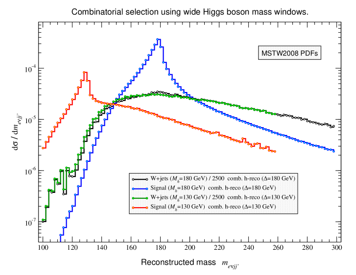
Figure 3 shows the spectra including shower effects for signals and backgrounds at and after the combinatorial Higgs boson reconstruction has been applied using wide Higgs boson mass windows (). The parton showering washes out the peaks, therefore reduces and broadens them. Both signal distributions develop a softer tail above as a result of the jet combinatorics. For , the tail plateaus due to the off-shell effects mentioned earlier. Figure 3 also illustrates why the value of the significance jumps up significantly (as shown in Figure 2) when we tighten the Higgs boson mass window from to for . This effect arises because we place our window cuts in a steeply rising +jets background.
When we studied which choice of mass window gives us the best results in terms of separating signal from background, it came as somewhat of a surprise that we did not have to alter the additional dijet mass constraint of , . Our studies indicate that it is helpful to have the hadronically decaying boson to be close to its on-shell mass . The boson decaying leptonically is then forced to go off-shell (), a kinematic configuration at odds with most +jets events.Cutting on therefore helps suppress the dominant background and, moreover, should also be convenient to demote the production of multi-jets efficiently.
For the tighter Higgs boson mass windows, our results show that a simple one-sided lower cut on , i.e. is slightly more efficient than using any type of dijet mass window. The one-sided cut improves the significances as given in Table 8 by 1–2%. The removal of the upper bound on has however negligible effects on selections using broad Higgs boson mass windows. As a consequence of keeping an constraint the leptonically decaying will almost always be off-shell, such that the reconstruction of the longitudinal component of the neutrino’s four-momentum cannot succeed without a good guess of the mass of the pair. We will address this issue in Section 4.3.
4.2.2 Effect of the subdominant backgrounds
In this section, we examine to what extent the significances of the ideal Higgs boson reconstruction will be diluted by contributions from the electroweak and top-pair production of the +jets final states. To this end we apply the analysis as established so far, without any modification.
The first thing to notice is the total inclusive LO cross sections for these minor backgrounds are – substantially smaller than the production contribution. After the application of the basic cuts, the inclusive +2-jet cross sections drop to about , a factor of 40 below the major background. Including all the various -factors, see Table 1 and Eqs. (17), (21), (22), we find that the total significance,
| (24) |
at the basic selection level is only 2% smaller compared to the significance using only +jets.121212The cross sections stated are LO-like cross sections as obtained with SHERPA: before (after) the basic cuts, we find and ( and ) for the electroweak and backgrounds, respectively; the resulting single-background significances turn out to be almost 6 and 10 times larger than the +jets .
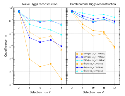
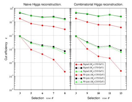
Switching from the baseline selection to a combinatorial selection and finite dijet mass window, the single minor-background significances improve by up to 50% above (100% below) the threshold. So, for beyond-baseline reconstructions, the significance corrections owing to the inclusion of the minor backgrounds will be of the same order as before. This is documented in both Figures 4 and 5. In the former we compare the cut efficiencies between all backgrounds and the signal (shown together with the +jets background in the plots to the right in Figure 4) for various naive and combinatorial Higgs boson candidate selections. Firstly, no background cut efficiency ever exceeds any of the . In all cases the background curves decrease more strongly when tightening the selection. Secondly, the pattern we observe for the minor-background cut efficiency curves resembles by and large those of the major background.131313In particular, the minor-background cut efficiencies show more pronounced drops, if one enhances the baseline to a Higgs boson candidate selection, introduces the dijet mass window or tightens the Higgs boson mass range. Notice that the naive Higgs boson reconstruction very efficiently beats down the background. This is because the two leading jets turn out harder compared to all other cases. The presence of a sufficient number of subleading jets however makes the selection based on jet combinatorics pick a pair of soft jets, and, on the contrary almost too effective for Higgs boson masses above the threshold. For these reasons, the single-background significances plotted versus follow the trend found for the +jets contribution, but remain well above the +jets significances.141414Both the electroweak and production significances show the same strong enhancement around as a result of the effect discussed around Figure 3 which is due to the use of a tight Higgs boson mass window. As for +jets, the minor backgrounds fall rapidly for decreasing . All of which is exemplified in Figure 5 using three Higgs boson candidate selections, which impose a dijet mass window (corresponding to the rows 8, 11 and 13 in Tables 4, 7 and 10), namely the naive method with (left panel) and the combinatorial method with the same and broader window of (middle panel). The total significances resulting from combining the three single backgrounds are also shown. In fact, they only decrease by 1–5% as demonstrated by the ratio plots in the lower part of Figure 5. The high region is found to receive the larger, corrections once the electroweak and contributions are included in the overall background. As noted early in Section 3.2, experimenters have estimated this fraction of events with 5% implying a 2.5% drop in significance. It is reassuring to be able to confirm this expectation with our results. Slightly contrary to the expectation, we identify the electroweak as the leading minor background in all selections.
Based on these results it is easy to conclude; at this stage of our analysis we do not have to worry about contributions from minor backgrounds. Although additional handles exist to further reduce these backgrounds or supplement the (here conservatively chosen) -jet veto, it is of far more importance to find ways to diminish the +jets background. We postpone this discussion until Section 4.4.
4.3 More realistic Higgs boson reconstruction methods
Up to this point we have ignored one big problem, namely the neutrino problem. In our selection based on the reconstruction of invariant masses – which we dubbed invm approach – we currently treat neutrinos as if we were able to measure them like leptons. This is, of course, unrealistic and before we can talk about further significance improvements, we have to investigate in which way our analysis may fall short when switching to more experimentally motivated Higgs boson candidate selections. Under experimental conditions, missing energy is taken from the imbalance in the event. However, in our analysis we then make a small simplification and identify the missing energy with the neutrino’s transverse momentum as given by the Monte Carlo simulation.
There are multiple choices for how to proceed.Recall that whatever method we pick acts as a selection criterion; we decide which two jets to keep in the event based on these variables, therefore we want to design variables, which are best at correctly picking out the jets from a Higgs boson decay. One way to proceed is to give up complete reconstruction and to work solely with transverse quantities; this is clean and unambiguous, but we throw out information. The second approach is to attempt to guess the longitudinal neutrino momentum by requiring that some or all of the final-state objects reconstruct an object we expect, such as a or Higgs boson. Full reconstruction then gives access to a larger set of observables, therefore keeps more handles and information, but it is also more ambiguous.
| pzmw | pzmh | mt | mtp | |||||
|---|---|---|---|---|---|---|---|---|
To remove some of the combinatorial headache, we use and (transverse) mass windows as before; moreover, we can impose criteria on subsets of the event. For example, if the (3-particle) mass of the visible system is greater than the test Higgs boson mass, that particular choice of jets is unphysical and we can move on to the next choice. A second constraint we often impose is that the 4-particle transverse mass does not exceed the upper bound on the Higgs boson mass window: . As to the definition of , we generally use the definitions stated in Section 2, see Eqs. (8) and (9). For our selections, we found that the distinction of the two definitions in fact only matters when we calculate the 4-particle transverse masses. Accordingly, each selection comes in two versions either using or . In Table 5 we summarize for each type which version is more appropriate to use and in what context. Whenever we refer to a specific selection in due course, we understand it according to the findings listed in Table 5.
With these criteria in hand, the different selection methods are specified as follows:
-
•
mt: we want to test a method where the final state of the Higgs boson decay will be identified purely with the help of transverse masses rather than invariant masses. To this end we calculate according to Eqs. (8) or (9) and prefer the final state giving us the 4-particle transverse mass closest to . Owing to the test mass window is placed on the lower side only, , with double the size as compared to the other selections. The advantage, but also disadvantage of the method is there is no reconstruction. Avoiding reconstruction eliminates uncertainties owing to constraining masses plus resolving ambiguities, but means we have no access to longitudinal and invariant-mass observables involving the neutrino.
For the next two selections, we aim to approximately determine the longitudinal momentum of the neutrino, , using knowledge about which value for should likely be reconstructed by the combined system,.151515Provided the MET cut was passed, we assume here that all MET in the event has been produced by a single neutrino. When we write
| (25) | |||||
using the “(in)visible” subsystem notation, we note that such problems can be solved up to a twofold ambiguity. The difference among the two selections lies in how particles are grouped in Eq. (25) and how the twofold ambiguity is resolved.161616If the solutions are complex-valued, we only assign the real part to describe with no ambiguity left to resolve.
-
•
pzmw: in this selection we use the mass constraint to solve for the neutrino momentum: . The ambiguity is then resolved by picking the neutrino solution, which brings the reconstructed mass more closely to the Higgs boson test mass . For true signal events, it then is more likely to find the reconstructed matching the Higgs boson mass.
The tricky part is to pick the best choice for the constraint – meaning is always optimal given that the boson may be off-shell? For pzmw, we do the following: first, we inspect the transverse mass, , of the subsystem in each event. If we choose , otherwise we pick as long as or . That is, above and around the threshold, we take towards . If below threshold and , the mass estimate is chosen taking various subsystem invariant and transverse masses into account but enforcing to lie between and . For example, if we set while otherwise unless where we say .
-
•
pzmh: we again infer the neutrino’s longitudinal momentum from mass constraints. Although technically similar to pzmw – with the “visible” subsystem entering Eq. (25) now being – we here turn the idea around and already require in order to solve for . That is to say we enforce the combined system, , to mimic a Higgs boson signal mass while leaving us with reasonable leptonic masses at the same time. When reconstructing the signal these observables are likely correlated, while for the background they are uncorrelated apart from kinematic constraints.
The details of the method are: we specify the target mass via unless we find , i.e. the 4-particle transverse mass turns out too large already so that is the more appropriate choice. We approximate the leptonic boson mass by freezing it at if this difference exceeds . We however require . Taking this estimate, we can form the absolute difference using the reconstructed mass for each possible neutrino solution. In the presence of two solutions we define, as a measure of the longitudinal activity, with and pick the solution that generates the smaller , i.e. the subsystem less likely going forward. We do so unless the other solution’s drops below and is satisfied; this is when we pick conversely ( if otherwise ). Finally, we ensure that the set minimizing will be preferred by the overall selection among all sets reconstructing the same 4-particle mass. Note that we do not reject the selected ensemble if the deviation becomes too large; we leave this potential to be exploited by supplemental cuts, which we discuss in Section 4.4.
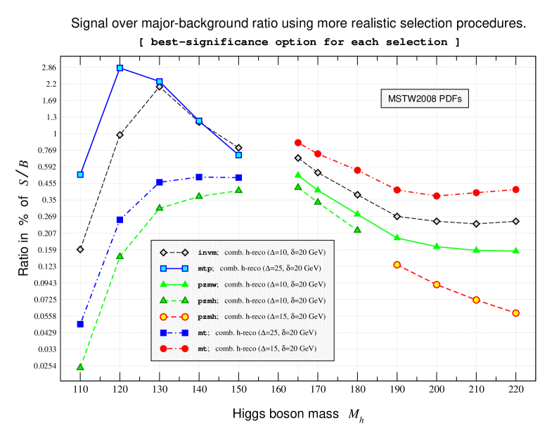
We explored in detail how each of these selection criteria compare to the ideal case. Figure 6 shows the significances per test point that we can achieve running the different combinatorial selections for various, reasonable window parameters. In the upper panels we display them directly on top of the (quasi optimal) ideal case, i.e. the invm combinatorial candidate selection. The plots on the right and in the center respectively exhibit the results of the mt and pzmh methods for the whole test range. The pzmw method yields similar, yet slightly worse results below the mass threshold compared to pzmh. Therefore, we split the leftmost pane into two subplots: on the right, one finds the pzmw results for masses above threshold; on the left we then already reveal the outcome of the mtp selection, whose discussion we postpone until the next subsection.
The bottom-row plots of Figure 6 depict the respective survival fractions: the significance ratios for each selection and different window parameters always taken with respect to the quasi optimal case (cf. the thick lines with symbols). To indicate the net effect of the more realistic approaches, we also show in each case the significance loss relative to the invm selection using exactly the same mass windows as the realistic one (cf. the thin lines with no symbols). We observe serious losses, larger than 50%, if one uses selections with tighter window parameters and/or runs for points further away from . The reconstruction methods (pzwm, pzmh) do not work better than 90% of the quasi optimal case. This only is improved by the mt approach making use of broad Higgs boson mass windows where one can reach up to about 100%. However, lowering here quickly results in losing sensitivity. Related to the quasi optimal invm selection, the various results point us to work with medium-sized Higgs boson mass windows always imposing the dijet mass cuts. Tighter constraints may help improve the outcome of the reconstruction types, but are of disadvantage in the measurement.
In all selections the below-threshold region is especially problematic. One might settle for 65–80% of the ideal significances, but if we want to get a better handle on the low boson masses, in particular include the mass point, we have to push further – which we do so in Section 4.3.1.
Focusing on the above-threshold region, we see that pzmw slightly outperforms pzmh over the whole range; only for the near-threshold region up to this is topped by the mt selection for medium-sized windows. This is somewhat surprising, but seems plausible, if one considers that signal events are central in rapidity and manifest themselves in larger transverse activity on average. This has to be opposed to the +2-jets background whose events tend to populate phase space more along the beam direction, which generates distributions peaking about half an unit away from zero rapidity. Nevertheless the differences between the 3 methods are not conclusive per se; to some extent the selections will shape distributions differently and it is easy to imagine the picture changing if additional cuts are imposed. But, one has to bear in mind, there is a second, very important criterion, the ratio , which one wants to maximize. For their optimal window parameters, we show in Figure 7 the curves of the more realistic and ideal selections as functions of . Even more surprisingly than before, the mt outperforms the neutrino reconstruction methods and, moreover, the ideal are also beaten unless . Based on this observation one may prefer the methods where the selection utilizes transverse masses, with the only drawback of having no estimate available.
4.3.1 More realistic reconstruction below the on-shell diboson mass threshold
We have just seen that the significances achievable in more realistic scenarios drop off considerably below the mass threshold, amplifying the loss already present in the ideal case. Therefore, it is of great importance to learn how the reconstruction methods described above can be applied more efficiently in the below-threshold region.
We noticed that the mt selection picks up background events, which often fall outside (mostly above) the Higgs boson mass window. As a result, a somewhat different class of background events survives the mt selection procedure compared to utilizing the invm, ideal, approach. This is no surprise since we have already argued that the Higgs boson decays yield an enhanced transverse production with regard to the +2-jet background. Using , Figure 8 exemplifies this by means of the and ratio distributions. We clearly see the large impact on the +jets results being a consequence of enforcing a transverse- rather than invariant-mass window. Imposing the constraint on the background is fairly equivalent to choosing events with larger longitudinal components. This drives the associated invariant masses to higher values whereas the ratios are shifted to lower ones.
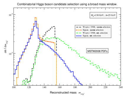
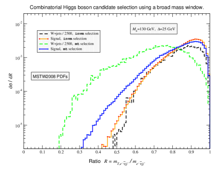
To give a more quantitative example, we consider the case for broad (tight) Higgs boson mass windows and . If we select events using mt, then discard all those events with an invariant mass outside , we find a quite impressive gain of 82% (360%). Similarly, if we use the invm selection and apply further cuts removing events with values greater than or less than , we observe that improves by 12% (drops by 20%). As the invm selection has a better starting than mt, the final significances are similar in all cases, however the essential point is we can improve the significance by combining the transverse- and invariant-mass selections.
To exploit this potential in a more realistic scenario, we use (in a first phase) the mt selection to pick out the 4-particle system, then (in a second phase) reconstruct the neutrino momentum following the pzmw procedure. Compared to the ideal case, this reconstruction works rather inefficiently in identifying background events that yield invariant masses . As it is optimized to the features of the Higgs boson decay signal, pzmw generates estimates by assuming ratios close to 1. For +jets, these choices often turn out to be sufficiently smaller than the actual masses of the leptonically decaying boson. The +jets background usually contains an on-shell , a lower is not ideal and tends to bring down the deconstructed, associated 4-particle masses . As a result a good fraction of background events possessing true invariant masses exceeding the upper bound on (see left plot of Figure 8) are shuffled back into the Higgs boson mass window.
Hence, we make adjustments to the pzmw reconstruction used in this symbiosis of selections so that it performs better below threshold. The basic idea is to maximally exploit the differences of signal and background in the leptonic and hadronic mass distributions. If, after initial mt selection, we constrain the transverse masses of the and dijet subsystems by placing cuts that favor and , we enforce off-shell decays while keeping those of on-shell. This is beneficial to the signal and suppresses, at the same time, the +jets background. Here, we only add requirements on the hadronic subsystem by imposing a minimum value for . We leave the potential to be exploited by the -dependent cut optimization (which we discuss in Section 4.4), since demanding an upper bound on would not only enhance mt but all realistic selections.
With this major adjustment, we can now design a promising mt+pzmw selection, which we call mtp:
-
•
mtp: the very first part of computing is identical to the mt selection. Subsequently, we require to be greater than , which we have parametrized in terms of for convenience. This concludes the phase of testing the transverse criteria. Accepted candidates are subject to the neutrino reconstruction, whose implementation deviates from pzmw to some extent: we choose freezing it below ; here we employ but keep it constant above (). As in all other reconstruction methods we then solve for the longitudinal momentum of the neutrino, cf. Eq. (25), and reject the particular choice if the solutions are degenerate or generate a mean mass deviating from by more than .171717Here, we do not adopt tight choices owing to the uncertainties intrinsic to the reconstruction of the component. In all other cases, we pick the solution giving the smaller and accept it if the reconstructed mass falls inside the window around .
The mtp results we can reach in terms of significance and sensitivity are known already from Figures 6 and 7. The increase in (leftmost plot in Figure 6) and (Figure 7) is highly visible for all of the test masses below threshold. For the mtp analyses with broadest windows, the significance effect is huge compared to the respective ideal selections using the same parameter. Likewise the signal over background ratio turns out similarly or even better than in the quasi optimal case.
Not only does mtp profit from the better selection performance, but we end up with a fully reconstructed neutrino vector, giving us access to a larger set of observables. However, because of the hard cut on , we notice that the mtp-selected backgrounds are strongly sculpted, washing out a number of shape differences. The effect of the cut moreover deteriorates as soon as . We obtain significances similar to the other methods and since they sculpt the background less, there is no real advantage to applying mtp above threshold, hence, we restrict its use to the low-mass region. On that note, it remains to be studied whether the , improvements came at the expense of further handles for the -dependent optimization. As a possible consequence the mtp selection actually might be superseded by an – at this level – inferior selection once enhanced by appropriately designed cuts.
4.4 Optimized selection – analyses refinements and (further) significance improvements
Having established the more realistic overall picture, we here discuss steps to achieve better signal over background discrimination. After baseline and combinatorial selections, we are interested in cuts that help further increase the significances obtained so far, i.e. . Our aim is to identify observables for each test point that are sufficiently uncorrelated such that simultaneous selections yield a total significance gain in the range:
| (26) |
Above relation is written out for the example of two extra handles, but easily extensible to multi-cut scenarios. As we have shown, the subdominant backgrounds have negligible effects at this level; we therefore concentrate on reducing the +jets background, although the other backgrounds are still included in computing the total significance. In order to be conservative about mass resolutions for hadronic final states at the Tevatron, we will fix the mass window parameters as .
As we have done in earlier sections, we divide the optimized selection into three broad Higgs boson mass ranges: below threshold, near threshold, and above threshold. As we vary the Higgs boson mass, we probe different kinematic configurations for the background. For the lowest Higgs boson mass, many background distributions (, , etc.) are steeply rising in the region of interest, cut off from below by baseline kinematics. For intermediate Higgs boson masses, the backgrounds tend to be flatter or peaked, while the higher Higgs boson mass region overlaps with backgrounds that are sharply falling. This basic shape behind (many) background distributions drives which cuts are optimal for a given Higgs boson mass. We present a number of distributions in Appendix B.2 to back up the many findings presented in this subsection.
The optimized analysis employs only observables constructed out of the momenta of the selected 4-particle system . More inclusive observables may be useful: for example, the scalar sum of the two selected-jet versus the two hardest-jet , . However such observables may also be subject to larger uncertainties from, e.g. the modeling of hard initial state radiation. To reduce these uncertainties one could extend the ME+PS program here, e.g. to inclusive +3-jets, however this is beyond the scope of this study.
In the optimized analysis the longitudinal observables, or , offer only moderate gains in significance (typically, we obtain gains on the order of 3–10% with larger gains occurring for heavy ), but they are insensitive to the exact value of the Higgs boson mass and are therefore more broadly applicable. The total 4-particle pseudo-rapidity can only be used in the pzmw, pzmh or mtp selections, since reconstruction of the neutrino is necessary. By the same logic, because the pseudo-rapidity difference between the selected jets is independent of the neutrino, cuts on can be used with all selections (though they are not efficient for mtp). We find that the requirements and work well for the entire range of Higgs boson masses we are interested in, so we include these cuts into our optimized (pzmh/w and mt) selection. In Appendix B.2 we present examples of distributions (Figure 12) and spectra (Figure 13) after un-optimized combinatorial selections, documenting the usefulness of these cuts.
The other useful observables we have found are all transverse, or in some cases based on invariant masses. Unlike the longitudinal variables, the optimal transverse variables and cut values depend strongly on the Higgs boson mass. We also find that transverse and longitudinal observables are largely uncorrelated in this study, so any gains in significance from selections in the transverse observables will add to the gains from and . We refer to Figures 14 and 15 of Appendix B.2 conveniently illustrating this decorrelation for the case versus .
| comb. -reco | leading = major cut | gain | subleading cut | gain | minor cut | gain | ||
| selection | ||||||||
| mtp | 17 | 9 | 4 | |||||
| mt | 70 | 52 | 6 | |||||
| pzmw | 73 | 38 | 10 | |||||
| pzmh | 63 | 59 | 48 | |||||
| mtp | 6 | 4 | 4 | |||||
| mt | 38 | 31 | 4 | |||||
| pzmw | 53 | 42 | 11 | |||||
| pzmh | 48 | 46 | 25 | |||||
| mtp | 8 | 3 | 3 | |||||
| mt | 24 | 15 | 6 | |||||
| pzmw | 30 | 30 | 6 | |||||
| pzmh | 29 | 28 | 14 | |||||
| mtp | 14 | 3 | * | |||||
| mt | 18 | 10 | * | |||||
| pzmw | 20 | 18 | 9 | |||||
| pzmh | 19 | 19 | 9 | |||||
| mt | 18 | 12 | 3 | |||||
| pzmw | 18 | 17 | 20 | |||||
| pzmh | 18 | 13 | 15 | |||||
| mt | 20 | 16 | * | |||||
| pzmw | 20 | 13 | 11 | |||||
| pzmh | 20 | 9 | 9 | |||||
| mt | 24 | 22 | * | |||||
| pzmw | 23 | 11 | 5 | |||||
| pzmh | 24 | 10 | 5 | |||||
| mt | 28 | 27 | * | |||||
| pzmw | 24 | 15 | 5 | |||||
| pzmh | 29 | 17 | 3 | |||||
| mt | 31 | 28 | 9 | |||||
| pzmw | 25 | 20 | 6 | |||||
| pzmh | 32 | 25 | 4 | |||||
| mt | 36 | 27 | 8 | |||||
| pzmw | 24 | 23 | 14 | |||||
| pzmh | 36 | 36 | 7 | |||||
| mt | 39 | 26 | 8 | |||||
| pzmw | 29 | 22 | 15 | |||||
| pzmh | 49 | 43 | 8 |
Below-threshold region:
For pzmw and pzmh, the reconstruction selections, the transverse mass of the 4-particle system, , and (for pzmw at low ) the transverse mass of the leptonic system, , are the best observables. This result is really just a reiteration of the fact that simple reconstruction selections work poorly for below-threshold Higgs bosons. In our effort to make pzmh/w more flexible and apply them to below-threshold scenarios, we have allowed the possibility for background configurations that are inconsistent with a single parent resonance – such as 4-particle systems with . Removing this inconsistent region results in gains of .
For mt, the transverse mass of the dijet system or the scalar sum formed with the selected jets, , are the most optimal, with improvements of . The former cut takes advantage of the fact that the signal jets originate in a (real or virtual) boson, while the background jets come primarily from ISR – information that is not exploited in the initial mt selection. Somewhat smaller gains come from cutting on the total selected system’s transverse momentum, .
For mtp, there is little optimization to be done. Much of the physics that is behind the optimal cuts in the pzmh/w or mt cases has already been incorporated into the selection process. Some improvement is possible by cutting out the region with very low 4-particle transverse momentum, .
Near-threshold region:
For Higgs boson masses close to the threshold, the 4-particle is the most powerful additional handle. In Higgs boson production, as in other colour-singlet resonance production, the distribution is cut off at low values by soft-gluon resummation, and falls off at high values because of parton kinematics. The result is a peaked distribution. The hard scale of the process, dictated by the Higgs boson mass, sets the initial ISR scale, thereby influencing where peaks. Since the Higgs boson is heavier than the boson, always peaks at higher values for the signal compared to production. Even though the dominant background for our study is +2-jets, rather than +0-jets, the argument still holds. The peak in for +2-jets is still governed by and continues to peak at lower values than the Higgs boson signal. Selection criteria change the tails of the background distribution, but do not affect the location of the peak. Cutting out the low- region, improvements on the order of 20% are possible. Distributions such as , the scalar sum of the two selected jets, or , the of the 4-particle system, also have potential discriminating power. Signal versus background distributions in the relevant variables after baseline combinatorial selections are shown in Figure 17, see Appendix B.2.
Above-threshold region:
For higher Higgs boson masses, the total amount of (transverse) energy in the + system becomes the most powerful discriminator between the signal and the background. Specifically, once , the of the selected 4-particle system peaks at significantly higher values than the background, regardless of the selection technique. By cutting away the low- region, we find gains of order 25% are possible. The 4-object remains a very useful observable, as does the 4-particle transverse mass. Examples of signal versus background distributions are shown in Figure 18, see Appendix B.2.
Results:
The optimal or “leading” or “major” cuts for the different Higgs boson mass categories and selection methods are summarized in Table 6. To give some idea how useful the single best discriminator is compared to other observables, we also show the percent increase in significance for the second best or “subleading” single discriminator. Separately we have also determined which combinations of the leading discriminator (supplemented by the respective pseudo-rapidity cuts discussed above) with a second observable give the largest (additional) increase in significance. The second “minor” cuts of these optimal two-variable selections are summarized in the last two columns of Table 6. Note that in most cases these minor cuts do not involve the same observables as the subleading cut; this is because the subleading discriminator is typically strongly correlated with the leading discriminator, and thus does not add much to the combined significance. Some ideas beyond the application of minor cuts exist; we comment in Appendix B.3 on a few possible routes one can take to enhance the optimized analyses presented here.
When looking for minor cuts, we found in addition to variables we have already discussed, such as (in Section 2), and the 4-object , a few other observables, namely , and to be beneficial. The first two, and are common, so we do not repeat their definitions here. The last minor cut observable, is defined through exhibiting yet another way of defining a transverse mass. The additional gains from the minor cuts are typically small, except close to the threshold and for the largest Higgs boson masses considered here. In particular for , the boost of the system in the reconstructed 4-object rest frame stands out as a helpful discriminator of secondary order; for more details, we refer again to Appendix B.2 and the discussion around Figure 19. Also, the dijet-system based handles, and yield fairly substantial extra gains, but only at low if we rely on the pzmh method. Once jets are picked stemming from the backgrounds, the strict mass reconstruction of the selected 4-object, as encoded in pzmh and amplified by the major cut given through , gives rise to the selection of less energetic , jets with preferred pair masses of . The observables and exploit this fact conveniently, hence facilitate such secondary improvements, as shown in Figure 19 for the example of .
\psfrag{Significance}[c][c][0.92]{ {Significance}\quad$S/\sqrt{B}$}\psfrag{Higgs boson mass}[c][c][0.92]{ {Higgs boson mass}\quad$M_{h}$}\includegraphics[clip,width=320.88116pt,angle={-90}]{illustrations/opt.sgfc.mh.2.ps}
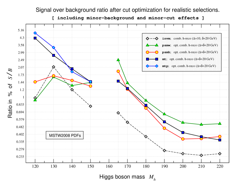
Finally, the baseline combinatorial and optimized combinatorial significances are displayed as a function of the Higgs boson mass in Figure 9. The ratio plots associated with each selection in the lower part of the figure visualize the significance increase achieved by the optimization. Independent of the selection, they also indicate a drop of significances caused by the subdominant backgrounds. Focusing on the ratios taken with respect to the ideal case (orange lines with circles), these ratio plots emphasize that the optimized mt(p) (transverse) and pzmw selections work best below and above the mass threshold, respectively. The related ratios presented in Figure 10 confirm these findings. They turn out to be rather small, as a consequence of maximizing the significance and trying to preserve most of the signal; both of which does not allow for imposing too restrictive cuts. Advantageously, the actual number of signal events, , present in this channel is not small. Except for the Higgs signal at (with expected events), the optimized analyses usually leave us with hundreds of signal events (50–300), if we assume an integrated luminosity of . Even the 25 signal events for are sufficient, particularly as increases to .
Clearly, as seen from Figure 9, the optimized significances for the four different Higgs boson reconstruction methods are very similar. The best significance is for Higgs boson masses close to the threshold, suggesting that it would be possible to achieve 95% confidence level exclusion in a stand-alone analysis. For a Higgs boson mass in the range , the optimized significance is between and . Given the additional improvements expected from a full multivariate analysis, this indicates that the semileptonic Higgs boson decay channel can make a significant contribution to Higgs boson exclusion in this mass range.
5 Conclusions, caveats, and prospects
We have presented a systematic study of the prospects for extending the Tevatron exclusion reach for a Standard Model Higgs boson by including the final states arising from semileptonic Higgs boson decays. We have used a realistic simulation of the Higgs signal and the relevant Standard Model background processes to exhibit the kinematic differences between the signal and background. We have used three qualitatively different approaches to extracting the event kinematics, one based on transverse observables and the others based on approximate even-by-event full reconstruction. We have shown that all three approaches give similar results when one optimizes selections based on several discriminating observables. The details of the optimization depend on the Higgs boson mass, and in particular on whether it is below, near, or above the threshold for decay to two on-shell bosons.
The optimized significances that we have achieved are not sufficient for stand-alone Higgs boson exclusion except in the most favorable case where the Higgs boson mass is close to threshold. However the sensitivities shown here are certainly promising as ingredients to a combined multi-channel analysis.
One important caveat is that the signal to background ratios for this type of analysis are fairly small, on the order of a percent, as illustrated in Figure 10. This means that Higgs boson exclusion is sensitive to relatively small systematic errors in the modeling of the backgrounds, notably the dominant background from +jets. However we have shown here that an experimental analysis has multiple over-constrained handles on the kinematic features of the data, providing extra cross-checks. In addition, the Higgs boson candidate selection employed here to identify the two jets from the Higgs boson decay is by design rather stable against effects from extra hard radiation; this reduces the uncertainty in the background modeling.
The techniques described here are applicable to Higgs boson searches at the CERN Large Hadron Collider. At 7 TeV center-of-mass collision energy, the Higgs boson production cross section increases by a factor of 30, while the +jets background increases by a factor of 20. With no hard upper limit of the amount of data available, one can use more restrictive selections and improve both the signal to background ratio and the overall significance. A recent analysis by the ATLAS collaboration [91] employed a 4-object invariant mass reconstruction and a dijet mass window similar to the baseline naive analysis used here, but applied to the heavy Higgs boson mass region . A CMS study [92] looked at the enhanced signal to background ratio provided by focusing on VBF production (and thus requiring two extra forward jets). Because of the large branching fraction, the semileptonic mode might prove to be observable at the LHC over a larger mass range than the dilepton mode; thus it could play a critical role in establishing the nature of electroweak symmetry breaking, in the event that the Higgs boson mass is 120 GeV.
Acknowledgments
We would like to thank Bogdan Dobrescu for many lively and stimulating discussions. We would also like to thank Thomas Becher, Li Lin Yang, Tanju Gleisberg, Frank Petriello, John Campbell and Ciaran Williams for their help in accomplishing necessary cross-checks. We are grateful to Frank Krauss and Frank Siegert, as well as all other members of the SHERPA collaboration for their continuous support. We gratefully acknowledge useful discussions with Bob Hirosky and Lidija Zivkovic, as well as Lance Dixon, Gavin Salam, Walter Giele, Rakhi Mahbubani, Patrick Fox and Agostino Patella.
Fermilab is operated by Fermi Research Alliance, LLC, under contract DE-AC02-07CH11359 with the United States Department of Energy.
Appendix A Appendix: Monte Carlo event generation
A.1 Leading-order cross sections
Here we briefly report on the tests we have done to convince ourselves of the correctness of the SHERPA leading-order cross section calculations. We found satisfactory or better agreement in all our cross-checks, which we briefly summarize here:
-
•
For the case of decays, we have compared SHERPA’s branching ratios with those obtained by multiplying the Hdecay results for given in Table 1 times the PDG literature numbers for . Using AMEGIC++’s mode of calculating partial widths of processes, we determined for the various Higgs boson masses and respective widths of Table 1. The differences seen are at most on the few-percent level.
-
•
With the explicit knowledge of the SHERPA branching fractions we were able to extract Higgs boson production rates at LO from the SHERPA signal cross section calculations according to
(27) The numbers that we obtained from this procedure compare well to numbers of other LO calculations, for example the LO rates as evaluated in MCFM or provided by Becher and Yang for verification purposes [93].
-
•
SHERPA LO rates were computed for both finite top masses and in the infinite top-mass limit. The ratio of the former over the latter cross section given as
(28) singles out the dependence on the top mass versus Higgs boson mass ratio, which is encoded by the function
(29) Note that attains unity as , while it vanishes for . Comparing the numerical cross section ratios with the analytical values for , we found excellent agreement over the entire Higgs boson mass range considered in this study.
A.2 NLO calculations versus CKKW ME+PS merging
When compared to NLO calculations, it is evident that SHERPA’s CKKW merging approach does not account for the virtual corrections to +jets in their entirety.181818For a brief summary of the basics of the CKKW merging, see Ref. [70]. For the current generation of SHERPA Monte Carlo programs, the ME+PS facilities have been extended to allow for truncated showering, which is a major refinement over the CKKW approach, see Refs. [76, 94, 95]. The only contributions enter through Sudakov form-factor terms at leading-logarithmic accuracy used in the parton shower and to reweight the tree-level matrix elements. The real-emission corrections however are included on a fairly comparable level with respect to full NLO calculations.191919More recent versions of SHERPA, from version 1.2.3 on, have been enhanced by the means to generate, for a number of important processes, events at the hadron level with a rate correct at next-to-leading order in [83, 84, 96]. To make this work, SHERPA relies on interfacing external one-loop amplitude generators like MCFM [61, 97], BlackHat [98, 99] or, more generally, via the Binoth Les Houches Accord [100]. Because of the complexity of the procedure, such improvements are not yet available for arbitrary processes, in particular the multi-jet final states we are interested in. Unless one decides for a fixed-scale choice at NLO, both approaches determine the strong-coupling scales dynamically, i.e. on an event-by-event basis, taking the kinematic configuration of the event into account. For all these reasons, it then occurs that the CKKW shapes of distributions emerge in many cases quite similarly to those evaluated at NLO, making an application of global -factors feasible.202020For example, in [25] a global -factor of magnitude with respect to the total inclusive cross section as measured by CDF [101] was applied to achieve a good agreement between the data and the SHERPA predictions for inclusive jet multiplicity and transverse momentum distributions. The treatment to fix the strong couplings is different when multiple scales are present. While at NLO the scales are set uniformly such that all factors obtain the same value, in the CKKW method they are set locally by the procedure itself, cf. [68, 102, 70] for example. This is known as reweighting, constituting the second component of the matrix-element reweighting of the CKKW method. The assignment of the scales proceeds hierarchically based on the splitting history, which is identified by the -jet cluster algorithm when applied to the initial matrix-element configuration considering physical parton combinations only. The nodal values found by the clustering can be interpreted as the relative transverse momenta of the identified splittings. They are then used as the scales for the strong-coupling constants replacing the predefined choice of the initial matrix-element generation. It would be interesting to see if a hierarchical scale setting can further stabilize NLO results, but no such reweighting has been completely worked out yet for NLO calculations.
Appendix B Appendix: Analysis side studies and additional material
| cuts & | ||||||||||
|---|---|---|---|---|---|---|---|---|---|---|
| selections | ||||||||||
| 96 | 75 | 61 | ||||||||
| 1.0 | 1.0 | 0.10 | 1.0 | 1.0 | 0.08 | 1.0 | 1.0 | 0.06 | ||
| lepton & | 12 | 95 | 78 | |||||||
| MET cuts | 0.564 | 0.45 | 0.08 | 0.566 | 0.45 | 0.07 | 0.570 | 0.45 | 0.05 | |
| as above & | 51 | 41 | 34 | |||||||
| jets | 0.465 | 0.0087 | 0.50 | 0.474 | 0.0087 | 0.40 | 0.483 | 0.0087 | 0.33 | |
| as above & | 77 | 60 | 50 | |||||||
| 0.257 | 0.0032 | 0.46 | 0.256 | 0.0032 | 0.36 | 0.258 | 0.0032 | 0.29 | ||
| naive -reco | 87 | 72 | 64 | |||||||
| 0.274 | 0.0030 | 0.50 | 0.274 | 0.0029 | 0.40 | 0.276 | 0.0027 | 0.34 | ||
| naive -reco | 0.0011 | 91 | 81 | |||||||
| 0.211 | 0.0018 | 0.49 | 0.211 | 0.0017 | 0.40 | 0.212 | 0.0016 | 0.34 | ||
| naive -reco | 0.0013 | 0.0011 | 0.0011 | |||||||
| 0.221 | 0.0016 | 0.56 | 0.217 | 0.0014 | 0.45 | 0.216 | 0.0012 | 0.40 | ||
| naive -reco | 0.0020 | 0.0019 | 0.0018 | |||||||
| 0.151 | 71 | 0.57 | 0.148 | 60 | 0.48 | 0.147 | 49 | 0.43 | ||
| comb. -reco | 0.0011 | 89 | 79 | |||||||
| 0.372 | 0.0033 | 0.65 | 0.375 | 0.0032 | 0.52 | 0.381 | 0.0029 | 0.45 | ||
| comb. -reco | 0.0017 | 0.0014 | 0.0013 | |||||||
| 0.258 | 0.0014 | 0.69 | 0.260 | 0.0013 | 0.56 | 0.262 | 0.0013 | 0.48 | ||
| comb. -reco | 0.0017 | 0.0014 | 0.0014 | |||||||
| 0.329 | 0.0019 | 0.77 | 0.329 | 0.0017 | 0.62 | 0.330 | 0.0015 | 0.55 | ||
| comb. -reco | 0.0023 | 0.0020 | 0.0020 | |||||||
| 0.284 | 0.0012 | 0.82 | 0.282 | 0.0011 | 0.68 | 0.282 | 88 | 0.61 | ||
| comb. -reco | 0.0027 | 0.0025 | 0.0024 | |||||||
| 0.237 | 83 | 0.82 | 0.234 | 71 | 0.69 | 0.233 | 59 | 0.62 | ||
| comb. -reco | 0.0030 | 0.0027 | 0.0027 | |||||||
| 0.209 | 67 | 0.81 | 0.207 | 57 | 0.68 | 0.206 | 47 | 0.61 | ||
| comb. -reco | 0.0033 | 0.0030 | 0.0030 | |||||||
| 0.146 | 42 | 0.71 | 0.143 | 35 | 0.60 | 0.142 | 29 | 0.54 | ||
| cuts & | ||||||||||
|---|---|---|---|---|---|---|---|---|---|---|
| selections | ||||||||||
| lepton & MET | 27 | 97 | 27 | |||||||
| cuts & jets | 0.0673 | 0.0087 | 0.027 | 0.104 | 0.0087 | 0.095 | 0.173 | 0.0087 | 0.27 | |
| naive -reco | 20 | 51 | 0.0011 | |||||||
| 0.00813 | 15 | 0.025 | 0.0276 | 44 | 0.11 | 0.0733 | 89 | 0.35 | ||
| naive -reco | 59 | 0.0029 | 0.0037 | |||||||
| 0.00261 | 16 | 0.024 | 0.0150 | 41 | 0.20 | 0.0444 | 17 | 0.49 | ||
| comb. -reco | 25 | 61 | 0.0013 | |||||||
| 0.0126 | 18 | 0.035 | 0.0389 | 51 | 0.15 | 0.0959 | 0.0010 | 0.43 | ||
| comb. -reco | 69 | 0.0028 | 0.0038 | |||||||
| 0.00374 | 19 | 0.032 | 0.0196 | 56 | 0.22 | 0.0587 | 21 | 0.58 | ||
| comb. -reco | 0.0016 | 0.0098 | 0.021 | |||||||
| 0.00181 | 40 | 0.033 | 0.0132 | 11 | 0.34 | 0.0382 | 24 | 1.11 | ||
| lepton & MET | 52 | 77 | ||||||||
| cuts & jets | 0.250 | 0.0087 | 0.51 | 0.328 | 0.0087 | 0.75 | ||||
| naive -reco | 0.0016 | 0.0018 | ||||||||
| 0.128 | 0.0015 | 0.63 | 0.188 | 0.0021 | 0.88 | |||||
| naive -reco | 0.0034 | 0.0035 | ||||||||
| 0.0795 | 42 | 0.73 | 0.130 | 76 | 1.00 | |||||
| comb. -reco | 0.0018 | 0.0022 | ||||||||
| 0.168 | 0.0017 | 0.78 | 0.247 | 0.0023 | 1.09 | |||||
| comb. -reco | 0.0038 | 0.0041 | ||||||||
| 0.109 | 51 | 0.91 | 0.180 | 89 | 1.28 | |||||
| comb. -reco | 0.012 | 0.0080 | ||||||||
| 0.0701 | 11 | 1.29 | 0.127 | 32 | 1.51 | |||||
B.1 Ideal Higgs boson reconstruction analyses
We first complete the presentation of our Section 4.2 main results by showing Tables 7 and 8 where we display the numbers associated with the high and low Higgs boson mass region, respectively. As in Table 4 we list the signal and +jet background cross sections, selection efficiencies, ratios and significances at different analysis levels. All cuts, the selection procedures, the layout of the tables and the interpretation of the results given in the tables have been discussed in detail in Section 4.2. Note that the rightmost column of Table 10 carries the outcomes for the test mass point .
One remark shall be added regarding the magnitude of off-shell effects. The loss one faces due to off-shell Higgs bosons can be read off Table 8 by comparing the acceptances after baseline (1st rows) and combinatorial Higgs boson selection (4th rows). While above the mass threshold the loss on the signal (background) is mild (significant) ranging from – (–), it steadily increases for decreasing , approaching and at and , respectively. The background loss factors turn huge (up to 48) because of the steeply falling spectrum (cf. Figure 3), but this cannot overcome the smallness of due to the signal reduction.
We now present the results of our side studies, which we decided to put in an appendix in order to not distract the flow of the main body.
| cuts & | ||||||||||
|---|---|---|---|---|---|---|---|---|---|---|
| selections | ||||||||||
| naive -reco | 0.0020 | 0.0018 | 0.0013 | |||||||
| 0.297 | 0.0022 | 1.14 | 0.296 | 0.0022 | 1.02 | 0.290 | 0.0023 | 0.77 | ||
| naive -reco | 0.0040 | 0.0032 | 0.0022 | |||||||
| 0.262 | 0.0010 | 1.50 | 0.258 | 0.0011 | 1.27 | 0.248 | 0.0012 | 0.92 | ||
| comb. -reco | 0.0024 | 0.0021 | 0.0016 | |||||||
| 0.370 | 0.0023 | 1.39 | 0.370 | 0.0024 | 1.22 | 0.368 | 0.0025 | 0.94 | ||
| comb. -reco | 0.0046 | 0.0037 | 0.0026 | |||||||
| 0.336 | 0.0011 | 1.83 | 0.337 | 0.0012 | 1.56 | 0.334 | 0.0014 | 1.16 | ||
| comb. -reco | 0.0076 | 0.0061 | 0.0043 | |||||||
| 0.257 | 51 | 2.07 | 0.258 | 57 | 1.76 | 0.255 | 64 | 1.30 | ||
| naive -reco | 92 | 76 | 67 | |||||||
| 0.287 | 0.0023 | 0.53 | 0.287 | 0.0022 | 0.42 | 0.288 | 0.0020 | 0.36 | ||
| naive -reco | 0.0015 | 0.0013 | 0.0012 | |||||||
| 0.240 | 0.0012 | 0.61 | 0.237 | 0.0011 | 0.49 | 0.234 | 91 | 0.44 | ||
| comb. -reco | 0.0011 | 90 | 80 | |||||||
| 0.368 | 0.0025 | 0.65 | 0.372 | 0.0024 | 0.53 | 0.375 | 0.0022 | 0.45 | ||
| comb. -reco | 0.0018 | 0.0015 | 0.0014 | |||||||
| 0.331 | 0.0014 | 0.79 | 0.331 | 0.0013 | 0.64 | 0.332 | 0.0011 | 0.57 | ||
| comb. -reco | 0.0030 | 0.0027 | 0.0027 | |||||||
| 0.251 | 61 | 0.89 | 0.248 | 53 | 0.74 | 0.247 | 44 | 0.66 | ||
The Higgs boson masses used in the analyses are, of course, hypothetical. However, we only considered the obvious scenario where the test mass has been set equal to the Higgs boson mass injected while generating the signal predictions. It is clear that one scans over a range of masses when pursuing an analysis, and here we do it in steps of 10 GeV; still the actual Higgs boson mass could deviate as much as 5 GeV from the assumed mass. Hence, we want to briefly study how strongly the invm Higgs boson candidate selections and their related significances depend on the match between the test and injected Higgs boson mass. To this end we generated other than default signal predictions for Higgs boson masses of and input them into the analyses using . Figure 11 shows the outcome of this side study where, for both types of analyses, we collected results for several mass window settings. We learn two things from plotting the significance as a function of the Higgs boson generation mass. First, the significances that we attain if we keep the selection parameters (, , ) constant are fairly robust over a broader range of generation masses. Yet the maximum occur for . Secondly we learn, asymmetric window placements such that are beneficial to achieve significance gains. By focusing on a single generation mass, e.g. , we see that the response in significance can easily get as large as 40%. The strong sensitivity can be understood by comparing the signal and background shapes as visualized in Figure 3 or the upper left plot of Figure 1.
| cuts & | ||||||||||
|---|---|---|---|---|---|---|---|---|---|---|
| selections | ||||||||||
| 14 | 14 | 51 | ||||||||
| 1.0 | 1.0 | 0.15 | 1.0 | 1.0 | 0.15 | 1.0 | 1.0 | 0.05 | ||
| lepton & | 18 | 18 | 65 | |||||||
| MET cuts | 0.560 | 0.45 | 0.12 | 0.573 | 0.45 | 0.13 | 0.572 | 0.45 | 0.05 | |
| as above & | 74 | 0.0013 | 29 | |||||||
| jets | 0.456 | 0.0087 | 0.72 | 0.275 | 0.0031 | 0.73 | 0.491 | 0.0087 | 0.28 | |
| as above & | 0.0013 | 0.0019 | 42 | |||||||
| 0.223 | 0.0024 | 0.67 | 0.136 | 0.0010 | 0.63 | 0.261 | 0.0032 | 0.25 | ||
| naive -reco | 0.0013 | 0.0030 | 58 | |||||||
| 0.276 | 0.0031 | 0.73 | 0.137 | 65 | 0.79 | 0.279 | 0.0024 | 0.30 | ||
| naive -reco | 0.0016 | 0.0037 | 75 | |||||||
| 0.214 | 0.0019 | 0.72 | 0.109 | 41 | 0.79 | 0.214 | 0.0015 | 0.30 | ||
| naive -reco | 0.0022 | 0.0038 | 0.0011 | |||||||
| 0.201 | 0.0013 | 0.83 | 0.115 | 42 | 0.82 | 0.216 | 99 | 0.37 | ||
| naive -reco | 0.0034 | 0.0056 | 0.0019 | |||||||
| 0.149 | 61 | 0.89 | 0.0825 | 21 | 0.84 | 0.147 | 40 | 0.39 | ||
| comb. -reco | 0.0015 | 0.0035 | 73 | |||||||
| 0.369 | 0.0034 | 0.94 | 0.175 | 70 | 0.98 | 0.385 | 0.0027 | 0.40 | ||
| comb. -reco | 0.0024 | 0.0056 | 0.0012 | |||||||
| 0.258 | 0.0015 | 0.99 | 0.121 | 31 | 1.02 | 0.266 | 0.0011 | 0.42 | ||
| comb. -reco | 0.0029 | 0.0046 | 0.0014 | |||||||
| 0.299 | 0.0015 | 1.15 | 0.154 | 47 | 1.05 | 0.332 | 0.0012 | 0.51 | ||
| comb. -reco | 0.0038 | 0.0060 | 0.0020 | |||||||
| 0.271 | 0.0010 | 1.26 | 0.135 | 32 | 1.11 | 0.282 | 72 | 0.56 | ||
| comb. -reco | 0.0045 | 0.0071 | 0.0025 | |||||||
| 0.230 | 71 | 1.27 | 0.114 | 22 | 1.12 | 0.233 | 48 | 0.57 | ||
| comb. -reco | 0.0049 | 0.0079 | 0.0027 | |||||||
| 0.204 | 58 | 1.25 | 0.102 | 18 | 1.11 | 0.206 | 38 | 0.56 | ||
| comb. -reco | 0.0054 | 0.0087 | 0.0030 | |||||||
| 0.142 | 37 | 1.09 | 0.0731 | 12 | 0.99 | 0.142 | 24 | 0.49 | ||
In the remainder of this appendix, we outline the impact of PDF variations and parameter variations other than , and on our analyses.
The SHERPA calculations resulting from using the CTEQ6.6 PDF libraries give a similar pattern with significances that are about 1–10% larger. This can be read off Table 9 and seen in Figure 2. By normalizing the Monte Carlo predictions for both PDF choices, MSTW2008 and CTEQ6.6, to the same respective theory cross sections, it is altogether reassuring to see that the cut and event selection procedures only induce deviations of the order of 10% or below. For the combinatorial Higgs boson candidate selection, one finds almost the same ratios, provided a wide Higgs boson mass window is used. The significances of the CTEQ6.6 calculations outperform those obtained with MSTW2008, once the mass windows for the Higgs bosons () and dijets () are tightened. We find the differences being more pronounced for Higgs boson masses just above the threshold.
Speaking of shape differences triggered by the use of different PDFs, we note that the MSTW2008 PDF set accounts for a larger transverse activity, i.e. rapidity distributions turn out steeper while the spectra develop 10–25% harder tails compared to the CTEQ6.6 predictions. Also, for MSTW2008, mass peaks are more washed out, again resulting in differences of the order of 25%.
Lastly, apart from the rightmost column, Table 10 gives more details for the choice including the cases where either the dijet mass window has been tightened from to or the threshold of the jet transverse momenta has been enhanced to .
B.2 More realistic Higgs boson reconstruction analyses
We collect here in this appendix additional material to substantiate our findings presented in Section 4.4. Figures 12–18 display a number of distributions resulting from the baseline plus combinatorial analyses. In each plot we show four curves, two predictions each for the signal and the +jets background as obtained after the ideal (invm) and one of the more realistic combinatorial selections. While we vary the Higgs boson masses and the choice of the realistic reconstruction method, we keep the window parameters of the combinatorial selections fixed at and over the whole set of spectra shown in these figures.
In Figure 19 we look at distribution taken at the intermediate optimization level, including the effects of the major cuts but before the application of the respective minor cuts as listed in Table 6. In these plots we compare the Monte Carlo predictions for the Higgs boson signals of different with all, dominant and subdominant background predictions. All these predictions follow from using realistic selection procedures where Higgs boson and dijet mass windows of have been employed.
Each one-dimensional distribution is supplemented by an one-minus-ratio subplot. The first prediction in the respective legend is always taken as the reference, which we have arranged to be a +jets prediction for all plots shown here. The ratio subplots nicely visualize why we place the cuts as given in Table 6. Note that in all plots we only compare the shapes, i.e. all distributions are normalized to unit area.
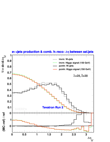
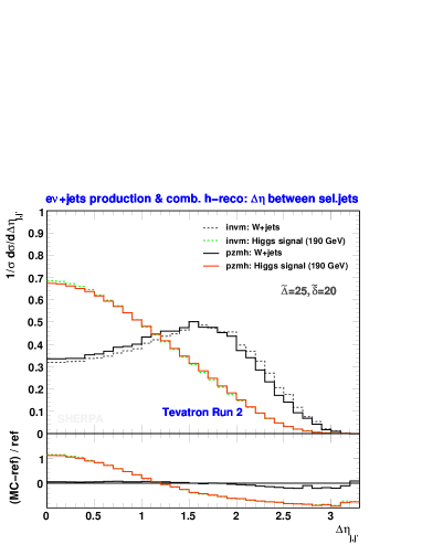
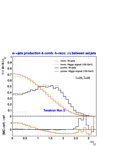
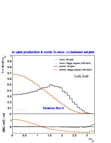
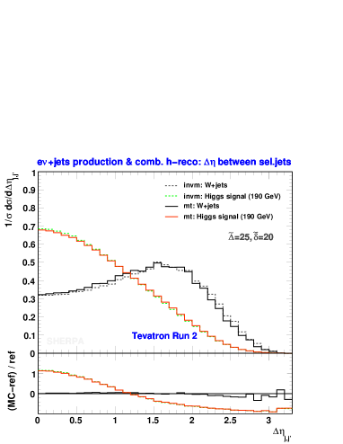
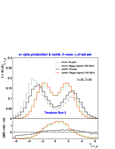
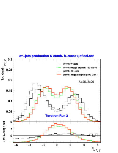
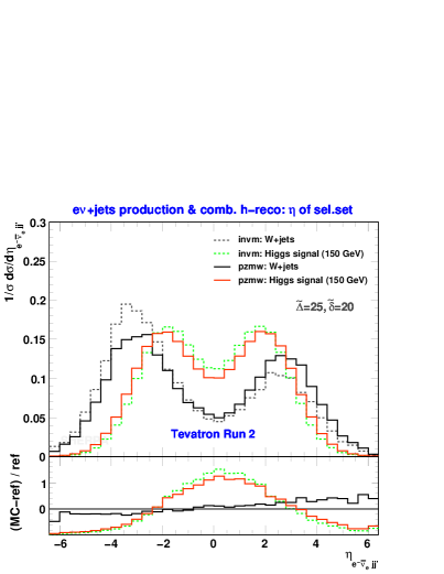
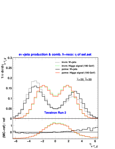
We start by showing the distributions in Figure 12. The differences in the results of the ideal and more realistic selections are immaterial; there are essentially no differences in the above-threshold cases. Furthermore, the shapes are very stable under variations. We see that placing a cut around keeps most of the signal, while it removes a large fraction of the +jets events. We note it is only the +jets background featuring a peak location away from zero, all other backgrounds (not shown here) behave similarly to the signal.
When working with the reconstruction methods, pzmh/w, we have access to another longitudinal variable: we can include a cut on the candidate’s pseudo-rapidity to supplement the constraints from the major and cuts. Figure 13 displays various distributions. Again, all predicted shapes are rather independent of the choice of the test mass . The +jets background (as well as the electroweak background which is not shown here) tends to preferably populate the forward rapidities while the signal (and the contribution also not shown here) shows up more central. This leads us to require as pointed out in Section 4.4 to achieve additional significance gains. Deviations between the ideal and more realistic reconstructions become visible; they now are , this is clearly because one needs information about the neutrino to form this observable. We observe that the +jets background receives the larger corrections compared to the signal.
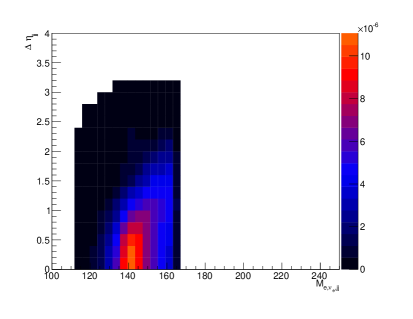
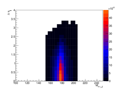
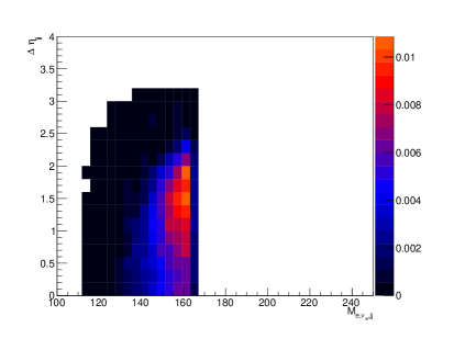
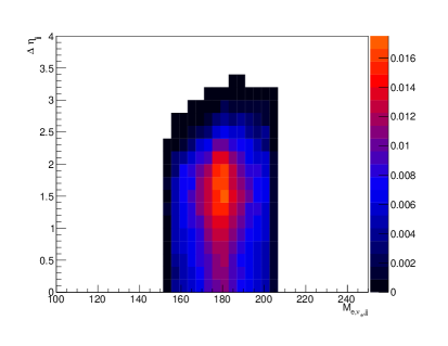
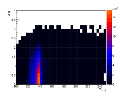
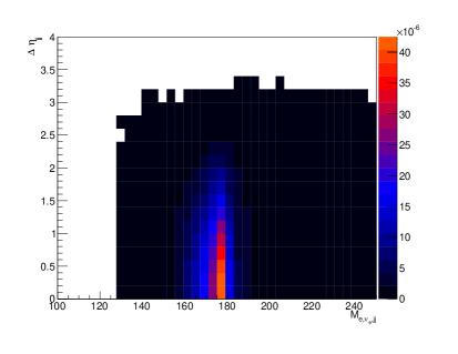
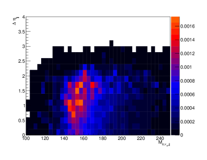
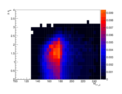
We add one more comment regarding longitudinal quantities. In this study, as stated in Section 4.4, the pseudo-rapidity variables, which we discussed above, occur largely uncorrelated with the transverse observables as well as invariant masses. Schematically, we illustrate this on the basis of two-dimensional versus distributions for both the Higgs boson signal and the +jets background. In Figure 14 we show these distributions as resulting from the combinatorial pzmw reconstruction for two different Higgs boson masses, below () and above () the diboson mass threshold. Similarly, Figure 15 exhibits the results obtained with the mt selection where the quantities were reconstructed as in the ideal case. When confronted with the respective +jets backgrounds, we notice that the predictions originating from the production of Higgs bosons cover rather different parameter regions in the – plane. This happens independent of the value of and the chosen combinatorial selection. Based on these observations, we expect the total increase to almost completely factorize into a product of single improvement factors.
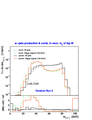
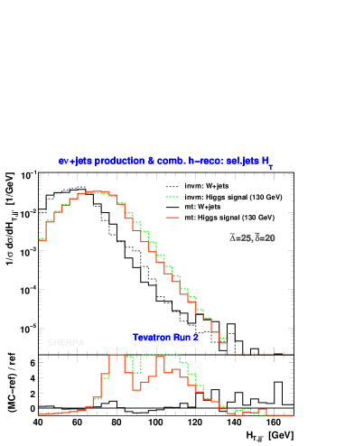
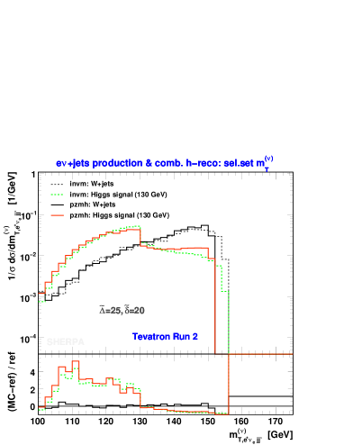
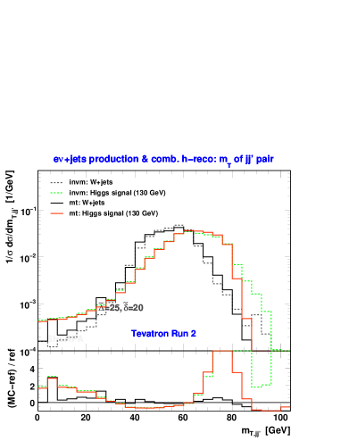
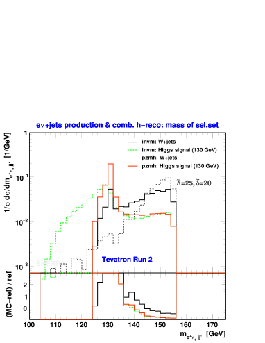
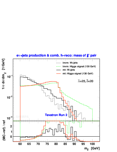
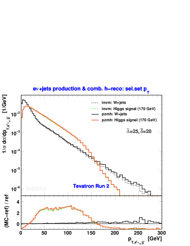
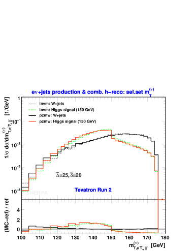
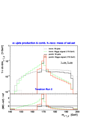
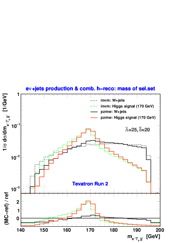
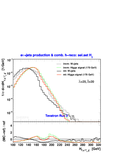
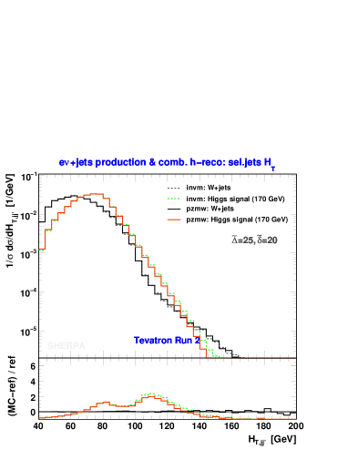
In Figure 16 we depict examples of potential discriminators below the diboson mass threshold. From the upper left to the lower right we present, for the choice of , the transverse mass of the leptonically decaying , the scalar sum of the selected jets, the transverse masses of the selected 4-particle set, , and of the selected jets, , as well as their corresponding invariant masses, and . The first three plots in that order are the leading cut variables for pzmw, mt and pzmh followed by the subleading cut variables for mt and pzmh, cf. Table 6. In the lower left plot we display the subsubleading cut variable for the mt method, , which would yield a significance gain of 19% if we were to demand . Unlike the transverse observables depicted in the upper and center panes of Figure 16, the invariant-mass distributions are affected by the modifications of the ideal selection owing to a realistic neutrino treatment. The selected 4-object invariant mass (lower left) exemplifies to what degree shapes can get distorted by the pzmh approach. The shoulder above emerges because complex solutions cannot be completely avoided in the reconstruction of the neutrino momenta; the lower tail arises from the constraints on the target mass , see Section 4.3.
The 2-particle transverse masses shown in the upper left and center right of Figure 16 together with the spectra document why we exploit the signal’s preference for on-shell hadronic and off-shell leptonic decays of the bosons. All backgrounds considered in this study disfavor this correlation. The 4-particle transverse mass (center left) exhibits – as expected – a nice kinematic edge for the signal at , while all backgrounds are continuous in this variable reaching their broad maxima above the applied mass window. The features of the handle (upper right) have been already described in Section 2. For this variable, the electroweak background turns out signal-like whereas the background generates (by far) the hardest tails.
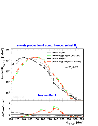
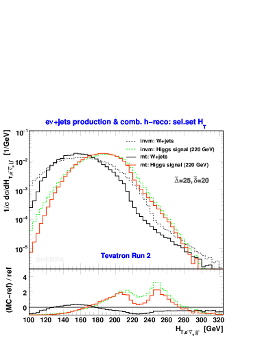
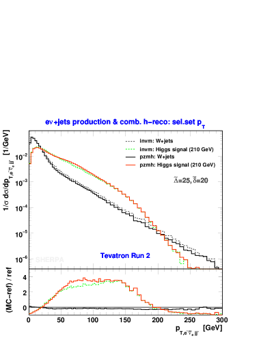
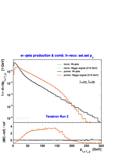
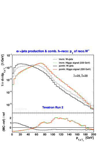
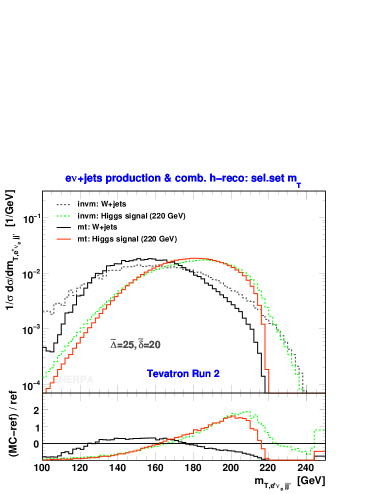
We now discuss some of the near-threshold discriminators where most of the examples are given for the test point . Figure 17 shows in its top row the two leading cut variables that we found for this mass region. In the upper right we have the transverse mass of the selected objects as resulting after the pzmw reconstruction with . We discover properties very similar to those discussed for the case of low Higgs boson masses, cf. Figure 16. In the upper left we have depicted the first-rank discriminator for medium Higgs boson masses – the selected 4-object transverse momentum distribution. It was introduced early on in Section 2. Here, we present the distribution as obtained after the combinatorial pzmh selection. We remark that the curves of the other two realistic approaches, pzmw and mt, (both not shown here) deviate even less from the respective curves of the ideal selection. Also not shown in Figure 17 but worthwhile to mention, the electroweak background would yield spectra similar to those of the +jets background whereas the top-pair production would turn up significantly harder than the signal’s spectra.
The other example plots of Figure 17 are chosen from the set of second-leading cut variables. The center panes display the invariant mass distributions resulting from the pzmh/w selections. As opposed to the – by construction – sculpted shapes of the pzmh method, we observe that the pzmw selection reproduces the invariant mass shapes of the invm ideal reconstruction to a large extent. The lower panes demonstrate the potential possessed by scalar transverse momentum sums that we exemplify by means of the selected-set observable as given by the mt selection (lower left) and the selected-jet observable resulting from the pzmw reconstruction (lower right). Remarkably, based on the 4-object , we can achieve an even clearer separation between the signal and the +jets background once we select candidates according to the mt method.
Figure 18 summarizes the types of discriminating observables as identified in Table 6 for the region of large Higgs boson masses; we use and in the example plots. The upper panels represent distributions obtained after pzmh (left) and mt combinatorial selections. Between these two cases we detect only marginal differences, and similarly between the predictions of the ideal and pzmw reconstructions (not shown here). At large Higgs boson masses, the signal develops the peak at considerably larger values compared to the +jets background. This characterizes the selected-set as the strongest handle we have above the threshold. Moreover, the pzmh and mt realistic selections further enhance the separation between the two peak regions. For the subdominant backgrounds (not shown here), we noticed a strong similarity between the spectra arising from the electroweak production and the +jets background. The background however yields the hardest spectra both in terms of the peak position as well as the tail of the distributions.
The center panes of Figure 18 show two examples of selected candidate distributions. These variables do not constitute the best discriminators anymore, but still quite often rank second best in separating signal from +jets production in the domain of large . As the pzmw reconstruction works extremely well for heavy Higgs boson decays into on-shell bosons, it gives shapes almost identical with the ideal selection.
For the point, we present two different subleading cut variables in the lower pane of Figure 18. To the left, one finds the distribution of the reconstructed resulting after selecting Higgs boson candidates according to pzmh. The purely transverse mass of the mt-selected 4-object set, cf. Eq. (8), is depicted on the lower right. For these variables, we recognize similar features as for the spectra concerning the minor backgrounds and the comparison with the invm Higgs boson candidate reconstruction.
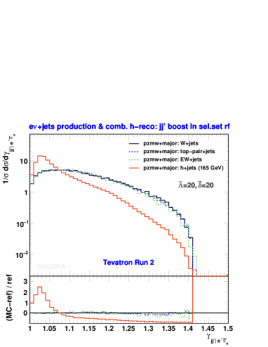
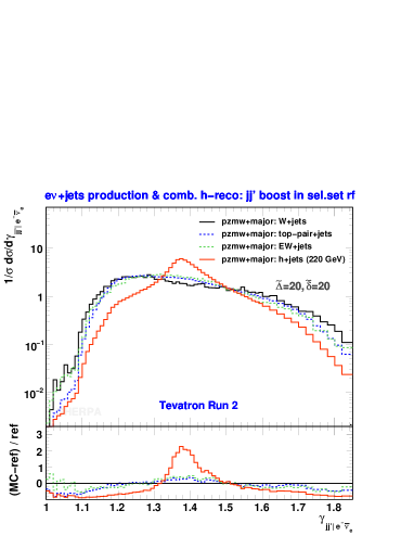
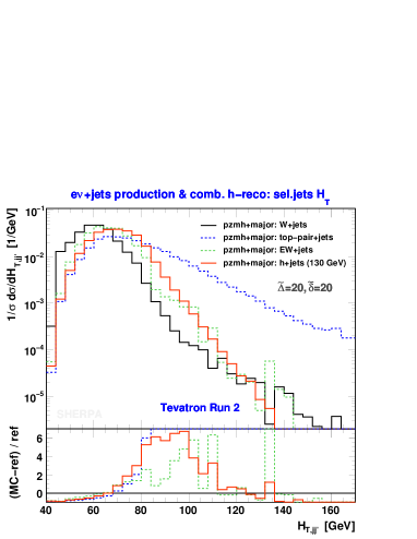
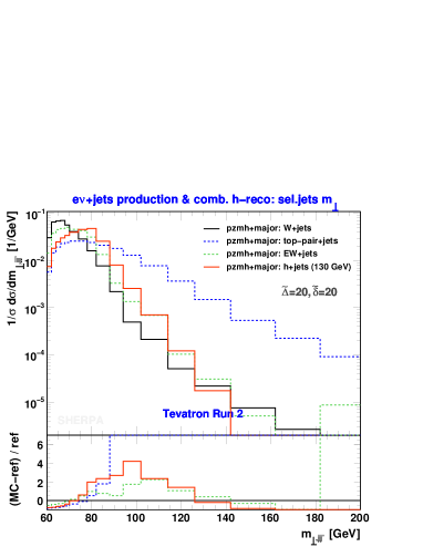
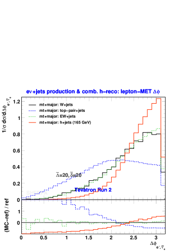
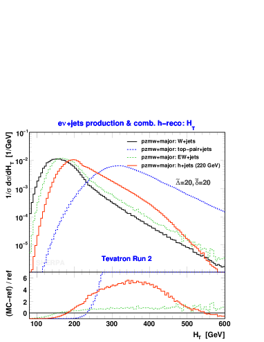
In Figure 19 we give a brief overview of discriminators that lead to a further increase in significance after implementing all major and rapidity constraints discussed in Section 4.4. The boost factor , as introduced in Section 2, proves very helpful in separating signal from backgrounds over a large range of above-threshold Higgs boson masses. Since develops a peak for the signal only, it is advantageous to isolate the boost factor peak region in order to exploit that a not too broad scalar resonance has been produced over a multitude of continuous backgrounds. This is exemplified in the upper plots of Figure 19 where we present two boost factor example distributions for (left) and when selecting via the pzmw method.
For the pzmh method in particular, we identified two transverse variables that, if constrained from below, are very yielding in the low Higgs boson mass region, even at this more involved level of the analysis. We exhibit these variables, on the left and on the right, in the center panes of Figure 19 choosing . As in similar cases the significance gain originates from exploiting the different peak locations associated with the signal, at higher values, and the dominant background, preferring the low values.
For very close above threshold, we can use the azimuthal angle between the lepton and MET or the two selected jets (as suggested by Han and Zhang in Ref. [7, 8]) to further suppress the backgrounds. A low- Higgs boson produced at threshold gives rise to two longitudinally moving bosons, which in turn each decay into two objects oriented almost back-to-back in the transverse plane. This is demonstrated by the example plot in the lower left of Figure 19 where signal and background distributions are shown for the observable when employing the mt selection for .
Finally, we display in the lower right of Figure 19 an example of a global-event observable, namely as calculated from the entire event, not vetoed by the selection and major cuts. It illustrates the hierarchy of scales intrinsic to the heavy Higgs boson signal () and different background processes; it also visualizes the leftover potential when considering the global for the implementation of additional cuts, see Appendix B.3.
B.3 Directions for additional improvements
The final sets of events surviving our optimized combinatorial selections of Higgs boson candidates are perfect for use as input to a full multivariate analysis. This is primarily because the analysis types presented here were geared towards significance maximization, so that a sufficiently large number of events can be preserved.
-
•
improvements: since we are rather safe from a statistics point of view, there is in many cases potential to improve by simply requiring more restrictive constraints accepting (mild) significance losses at the same time. The simplest way is to cut harder in the tails of the major observables; for instance for pzmw at , using (instead of the bound given in Table 6) results in a 40% gain in while the significance only drops by 10%. Of course, a change in variable sometimes is more beneficial for maximizing and keeping a reasonable significance. Consider for example mt at ; hardening the constraint by cutting out the region below maximizes by doubling it, but reduces the significance by a factor of . In contrast, using gives a factor increase in , yet only a factor decrease in significance. Certainly one can opt for the (other) extreme and totally maximize , e.g. for the pzmw case just mentioned, we find a huge gain of 600% by demanding but we actually just traded a reasonable significance associated with half a percent for a 4% of very low significance diminished by a factor of . This behaviour is typical owing to the limited amount of data taken at the Tevatron.
-
•
Overall cut: the philosophy of this study is to only constrain variables involving the candidate set of particles. Allowing cut observables sensitive to the whole event structure can lead to additional significance improvements but the related uncertainties are larger since such observables are more prone to hard radiative corrections that need to be described appropriately, often beyond parton-shower modeling. At the level of identifying minor cuts, as given in Table 6, we found that an overall cut on the selected events yields in most cases significance gains of the order of 20–40% near and above threshold. This is a conservative estimate considering the larger uncertainties on such cuts. An example is shown in the lower right of Figure 19 where we see why one benefits by constraining from below. In addition one could suppress the background by introducing an upper bound, or equally, exploit the fact that the leading jets in production yield a substantially harder spectrum.
-
•
Asymmetric mass windows for reconstruction methods: as touched during the discussion of Figure 11, the use of asymmetric test mass windows, i.e. , can improve the realistic selections that either approximate or set the selected 4-object mass, . For all values, it is advantageous to choose larger by a few GeV than where . The results presented in Figure 1 (upper left) and Figure 3 clarify why this is a good idea: first, the Higgs boson resonance is deformed by radiative losses and resolution effects (there is no perfect jet finding let alone (sub)event reconstruction) amounting to a larger portion of cross section below the peak; second, the backgrounds are either sufficiently flat or – below the threshold – steeply falling towards smaller masses amplifying the asymmetry effect further. We checked the asymmetric window scenario for the pzmw method, where this led to significance gains up to 10%. For the dijet mass windows, the effects turned out too weak.
References
- [1] M. Baak et. al., Updated Status of the Global Electroweak Fit and Constraints on New Physics, arXiv:1107.0975.
- [2] ATLAS Collaboration, Combination of the Searches for the Higgs Boson in 1 fb-1 of Data Taken with the ATLAS Detector at 7 TeV Center-of-Mass Energy, Tech. Rep. ATLAS-CONF-2011-112, CERN, Geneva, August, 2011.
- [3] CMS Collaboration, Combination of Higgs Searches, Tech. Rep. CMS-PAS-HIG-11-022, CERN, Geneva, 2011.
- [4] For CDF and DØ, the TEVNPH Working Group Collaboration, Combined CDF and DØ upper limits on Standard Model Higgs boson production with up to 8.6 fb-1 of data, arXiv:1107.5518. FERMILAB-CONF-11-354-E, CDF Note 10606 and DØ Note 6226.
- [5] On behalf of the CDF Collaboration, A. Buzatu, Standard Model Higgs boson search combination at CDF, in talk presented at the International Europhysics Conference on High Energy Physics, Grenoble, 21–27 July 2011.
- [6] On behalf of the DØ Collaboration, S. Greder, Combined upper limits on SM Higgs, in talk presented at the International Europhysics Conference on High Energy Physics, Grenoble, 21–27 July 2011.
- [7] T. Han and R.-J. Zhang, Extending the Higgs boson reach at upgraded Tevatron, Phys. Rev. Lett. 82 (1999) 25–28, [hep-ph/9807424].
- [8] T. Han, A. S. Turcot, and R.-J. Zhang, Exploiting decays at the upgraded Fermilab Tevatron, Phys. Rev. D59 (1999) 093001, [hep-ph/9812275].
- [9] Higgs Working Group Collaboration, M. S. Carena et. al., Report of the Tevatron Higgs working group, hep-ph/0010338.
- [10] W. Stirling, R. Kleiss, and S. Ellis, Pair Production in High-Energy Hadronic Collisions: Signal Versus Background, Phys. Lett. B163 (1985) 261.
- [11] J. Gunion, Z. Kunszt, and M. Soldate, A Background to Higgs Detection, Phys. Lett. B163 (1985) 389.
- [12] J. Gunion, P. Kalyniak, M. Soldate, and P. Galison, Searching for the intermediate mass Higgs boson, Phys. Rev. D34 (1986) 101.
- [13] J. Gunion and M. Soldate, Overcoming a Critical Background to Higgs Detection, Phys. Rev. D34 (1986) 826.
- [14] For CDF and DØ, the TEVNPH Working Group Collaboration, D. Benjamin, Combined CDF and DØ upper limits on and constraints on the Higgs boson mass in fourth-generation fermion models with up to 8.2 fb-1 of data, arXiv:1108.3331.
- [15] CDF Collaboration, T. Aaltonen et. al., Search for Production at CDF using 8.2 fb-1 of data, CDF Note 10599 (2011).
- [16] DØ Collaboration, V. M. Abazov et. al., Search for Higgs boson production in dilepton plus missing transverse energy final states with 8.1 fb-1 of collisions at = 1.96 TeV, DØ Note 6219-CONF (2011).
- [17] CDF and DØ Collaboration, T. Aaltonen et. al., Combination of Tevatron searches for the Standard Model Higgs boson in the decay mode, Phys. Rev. Lett. 104 (2010) 061802, [arXiv:1001.4162].
- [18] CDF Collaboration, T. Aaltonen et. al., Inclusive search for Standard Model Higgs boson production in the decay channel using the CDF II detector, Phys. Rev. Lett. 104 (2010) 061803, [arXiv:1001.4468].
- [19] DØ Collaboration, V. M. Abazov et. al., Search for Higgs boson production in dilepton and missing energy final states with 5.4 fb-1 of collisions at = 1.96 TeV, Phys. Rev. Lett. 104 (2010) 061804, [arXiv:1001.4481].
- [20] K. Iordanidis and D. Zeppenfeld, Searching for a heavy Higgs boson via the lepton neutrino jet jet mode at the CERN LHC, Phys. Rev. D57 (1998) 3072–3083, [hep-ph/9709506].
- [21] A. Djouadi, The Anatomy of electro-weak symmetry breaking. I: The Higgs boson in the standard model, Phys. Rept. 457 (2008) 1–216, [hep-ph/0503172].
- [22] B. Mellado, W. Quayle, and S. L. Wu, Feasibility of Searches for a Higgs Boson using + MET and High PT Jets at the Tevatron, Phys. Rev. D76 (2007) 093007, [arXiv:0708.2507].
- [23] B. A. Dobrescu and J. D. Lykken, Semileptonic decays of the standard Higgs boson, JHEP 1004 (2010) 083, [arXiv:0912.3543].
- [24] T. Gleisberg et. al., SHERPA 1.alpha, a proof-of-concept version, JHEP 02 (2004) 056, [hep-ph/0311263].
- [25] T. Gleisberg et. al., Event generation with SHERPA 1.1, JHEP 02 (2009) 007, [arXiv:0811.4622].
- [26] DØ Collaboration, V. M. Abazov et. al., A search for the Standard Model Higgs boson in leptons + jets in 5.4 fb-1 of collisions at = 1.96 TeV, DØ Note 6095-CONF (July, 2010).
- [27] DØ Collaboration, V. M. Abazov et. al., Search for the Standard Model Higgs Boson in the lepton + neutrino + Decay Channel, Phys. Rev. Lett. 106 (2011) 171802, [arXiv:1101.6079].
- [28] CMS Collaboration , according to CMS Statistics Committee, September, 2011.
- [29] F. Krauss, R. Kuhn, and G. Soff, AMEGIC++ 1.0: A Matrix element generator in C++, JHEP 02 (2002) 044, [hep-ph/0109036].
- [30] T. Gleisberg and S. Höche, Comix, a new matrix element generator, JHEP 12 (2008) 039, [arXiv:0808.3674].
- [31] For CDF and DØ, the TEVNPH Working Group Collaboration, Combined CDF and DØ upper limits on Standard Model Higgs boson production with up to 8.2 fb-1 of data, arXiv:1103.3233. FERMILAB-CONF-11-044-E, CDF Note 10441 and DØ Note 6184.
- [32] LHC Higgs Cross Section Working Group Collaboration, S. Dittmaier et. al., Handbook of LHC Higgs Cross Sections: 1. Inclusive Observables, arXiv:1101.0593.
- [33] M. Spira, QCD effects in Higgs physics, Fortsch. Phys. 46 (1998) 203–284, [hep-ph/9705337].
- [34] A. Djouadi, J. Kalinowski, and M. Spira, HDECAY: A program for Higgs boson decays in the Standard Model and its supersymmetric extension, Comput. Phys. Commun. 108 (1998) 56–74, [hep-ph/9704448].
- [35] Les Houches 2009 Tools and Monte Carlo Working Group Collaboration, J. M. Butterworth et. al., The Tools and Monte Carlo working group: Summary Report, arXiv:1003.1643.
- [36] A. Denner, S. Heinemeyer, I. Puljak, D. Rebuzzi, and M. Spira, Standard Model Higgs-Boson Branching Ratios with Uncertainties, Eur. Phys. J. C71 (2011) 1753, [arXiv:1107.5909].
- [37] Particle Data Group Collaboration, C. Amsler et. al., Review of particle physics, Phys. Lett. B667 (2008) 1.
- [38] C. Anastasiou, R. Boughezal, and F. Petriello, Mixed QCD-electroweak corrections to Higgs boson production in gluon fusion, JHEP 04 (2009) 003, [arXiv:0811.3458].
- [39] W.-Y. Keung and F. J. Petriello, Electroweak and finite quark-mass effects on the Higgs boson transverse momentum distribution, Phys. Rev. D80 (2009) 013007, [arXiv:0905.2775].
- [40] S. Actis, G. Passarino, C. Sturm, and S. Uccirati, NLO Electroweak Corrections to Higgs Boson Production at Hadron Colliders, Phys. Lett. B670 (2008) 12–17, [arXiv:0809.1301].
- [41] S. Actis, G. Passarino, C. Sturm, and S. Uccirati, NNLO Computational Techniques: The Cases and , Nucl. Phys. B811 (2009) 182–273, [arXiv:0809.3667].
- [42] D. de Florian and M. Grazzini, Higgs production through gluon fusion: updated cross sections at the Tevatron and the LHC, Phys. Lett. B674 (2009) 291–294, [arXiv:0901.2427].
- [43] S. Catani, D. de Florian, M. Grazzini, and P. Nason, Soft gluon resummation for Higgs boson production at hadron colliders, JHEP 0307 (2003) 028, [hep-ph/0306211].
- [44] S. Moch and A. Vogt, Higher-order soft corrections to lepton pair and Higgs boson production, Phys. Lett. B631 (2005) 48–57, [hep-ph/0508265].
- [45] A. D. Martin, W. J. Stirling, R. S. Thorne, and G. Watt, Parton distributions for the LHC, Eur. Phys. J. C63 (2009) 189–285, [arXiv:0901.0002].
- [46] For CDF and DØ, the TEVNPH Working Group Collaboration, Combined CDF and DØ upper limits on Standard Model Higgs boson production with up to 6.7 fb-1 of data, arXiv:1007.4587. FERMILAB-CONF-10-257-E, CDF Note 10241 and DØ Note 6096.
- [47] J. Baglio and A. Djouadi, Predictions for Higgs production at the Tevatron and the associated uncertainties, JHEP 1010 (2010) 064, [arXiv:1003.4266]. [Addendum arXiv:1009.1363].
- [48] J. Baglio, A. Djouadi, S. Ferrag, and R. Godbole, The Tevatron Higgs exclusion limits and theoretical uncertainties: A Critical appraisal, Phys. Lett. B699 (2011) 368–371, [arXiv:1101.1832].
- [49] J. Baglio, A. Djouadi, and R. Godbole, Clarifications on the impact of theoretical uncertainties on the Tevatron Higgs exclusion limits, arXiv:1107.0281.
- [50] V. Ahrens, T. Becher, M. Neubert, and L. L. Yang, Origin of the Large Perturbative Corrections to Higgs Production at Hadron Colliders, Phys. Rev. D79 (2009) 033013, [arXiv:0808.3008].
- [51] V. Ahrens, T. Becher, M. Neubert, and L. L. Yang, Renormalization-Group Improved Prediction for Higgs Production at Hadron Colliders, Eur. Phys. J. C62 (2009) 333–353, [arXiv:0809.4283].
- [52] V. Ahrens, T. Becher, M. Neubert, and L. L. Yang, Updated Predictions for Higgs Production at the Tevatron and the LHC, Phys. Lett. B698 (2011) 271–274, [arXiv:1008.3162].
- [53] C. Anastasiou, K. Melnikov, and F. Petriello, Higgs boson production at hadron colliders: Differential cross sections through next-to-next-to-leading order, Phys. Rev. Lett. 93 (2004) 262002, [hep-ph/0409088].
- [54] C. Anastasiou, K. Melnikov, and F. Petriello, Fully differential Higgs boson production and the di-photon signal through next-to-next-to-leading order, Nucl. Phys. B724 (2005) 197–246, [hep-ph/0501130].
- [55] F. J. Petriello , private communication, July, 2010.
- [56] P. M. Nadolsky et. al., Implications of CTEQ global analysis for collider observables, Phys. Rev. D78 (2008) 013004, [arXiv:0802.0007].
- [57] L. J. Dixon and M. Siu, Resonance continuum interference in the diphoton Higgs signal at the LHC, Phys. Rev. Lett. 90 (2003) 252001, [hep-ph/0302233].
- [58] T. Binoth, M. Ciccolini, N. Kauer, and M. Kramer, Gluon-induced WW background to Higgs boson searches at the LHC, JHEP 0503 (2005) 065, [hep-ph/0503094].
- [59] T. Binoth, M. Ciccolini, N. Kauer, and M. Kramer, Gluon-induced W-boson pair production at the LHC, JHEP 0612 (2006) 046, [hep-ph/0611170].
- [60] J. M. Campbell, R. Ellis, and C. Williams, Gluon-gluon contributions to W+ W- production and Higgs interference effects, JHEP 1110 (2011) 005, [arXiv:1107.5569].
- [61] J. M. Campbell and R. K. Ellis, MCFM – Monte Carlo for FeMtobarn processes. http://mcfm.fnal.gov.
- [62] J. M. Campbell and R. K. Ellis, Next-to-leading order corrections to + 2-jet and + 2-jet production at hadron colliders, Phys. Rev. D65 (2002) 113007, [hep-ph/0202176].
- [63] J. M. Campbell, R. K. Ellis, and D. L. Rainwater, Next-to-leading order QCD predictions for + 2-jet and + 2jet production at the CERN LHC, Phys. Rev. D68 (2003) 094021, [hep-ph/0308195].
- [64] S. Catani and M. Grazzini, An NNLO subtraction formalism in hadron collisions and its application to Higgs boson production at the LHC, Phys. Rev. Lett. 98 (2007) 222002, [hep-ph/0703012].
- [65] M. Grazzini, NNLO predictions for the Higgs boson signal in the and 4 decay channels, JHEP 02 (2008) 043, [arXiv:0801.3232].
- [66] S. Catani, F. Krauss, R. Kuhn, and B. R. Webber, QCD Matrix Elements + Parton Showers, JHEP 11 (2001) 063, [hep-ph/0109231].
- [67] F. Krauss, Matrix elements and parton showers in hadronic interactions, JHEP 08 (2002) 015, [hep-ph/0205283].
- [68] F. Krauss, A. Schälicke, S. Schumann, and G. Soff, Simulating + jets production at the Tevatron, Phys. Rev. D70 (2004) 114009, [hep-ph/0409106].
- [69] F. Krauss, A. Schälicke, S. Schumann, and G. Soff, Simulating + jets production at the CERN LHC, Phys. Rev. D72 (2005) 054017, [hep-ph/0503280].
- [70] J. Alwall et. al., Comparative study of various algorithms for the merging of parton showers and matrix elements in hadronic collisions, Eur. Phys. J. C53 (2008) 473–500, [arXiv:0706.2569].
- [71] J. Winter, QCD jet evolution at high and low scales. PhD thesis, Technische Universität Dresden, 2008.
- [72] P. Lenzi and J. M. Butterworth, A study on Matrix Element corrections in inclusive production at LHC as implemented in PYTHIA, HERWIG, ALPGEN and SHERPA, arXiv:0903.3918.
- [73] Les Houches 2009 SM and NLO Multileg Working Group Collaboration, J. R. Andersen et. al., The SM and NLO multileg working group: Summary report, arXiv:1003.1241.
- [74] DØ Collaboration, V. M. Abazov et. al., +jet production in the DØ experiment: A comparison between data and the PYTHIA and SHERPA Monte Carlos, DØ Note 5066-CONF (March, 2006).
- [75] DØ Collaboration, V. M. Abazov et. al., Measurement of differential + jet + X cross sections in collisions at = 1.96 TeV, Phys. Lett. B669 (2008) 278–286, [arXiv:0808.1296].
- [76] S. Höche, F. Krauss, S. Schumann, and F. Siegert, QCD matrix elements and truncated showers, JHEP 05 (2009) 053, [arXiv:0903.1219].
- [77] DØ Collaboration, V. M. Abazov et. al., Measurements of differential cross sections of + jets + X events in proton anti-proton collisions at = 1.96 TeV, Phys. Lett. B678 (2009) 45–54, [arXiv:0903.1748].
- [78] DØ Collaboration, V. M. Abazov et. al., Measurement of + jet + X angular distributions in collisions at = 1.96 TeV, Phys. Lett. B682 (2010) 370–380, [arXiv:0907.4286].
- [79] DØ Collaboration, V. M. Abazov et. al., Measurement of the normalized transverse momentum distribution in collisions at = 1.96 TeV, arXiv:1006.0618.
- [80] C. F. Berger et. al., Next-to-Leading Order QCD Predictions for + 3-Jet Distributions at Hadron Colliders, Phys. Rev. D80 (2009) 074036, [arXiv:0907.1984].
- [81] C. F. Berger et. al., Next-to-Leading Order QCD Predictions for + 3-Jet Distributions at the Tevatron, arXiv:1004.1659.
- [82] T. Gleisberg, F. Krauss, A. Schälicke, S. Schumann, and J. Winter, Studying production at the Fermilab Tevatron with SHERPA, Phys. Rev. D72 (2005) 034028, [hep-ph/0504032].
- [83] S. Höche, F. Krauss, M. Schönherr, and F. Siegert, Automating the POWHEG method in Sherpa, JHEP 1104 (2011) 024, [arXiv:1008.5399].
- [84] S. Höche, F. Krauss, M. Schönherr, and F. Siegert, NLO matrix elements and truncated showers, JHEP 1108 (2011) 123, [arXiv:1009.1127].
- [85] CDF Collaboration, T. Aaltonen et. al., Measurement of the + Production Cross Section Using the Lepton + Jets Final State at CDF II, Phys. Rev. Lett. 104 (2010) 101801, [arXiv:0911.4449].
- [86] DØ Collaboration, V. Abazov et. al., Measurement of trilinear gauge boson couplings from events in p anti-p collisions at = 1.96 TeV, Phys. Rev. D80 (2009) 053012, [arXiv:0907.4398].
- [87] J. M. Campbell and R. K. Ellis, An update on vector boson pair production at hadron colliders, Phys. Rev. D60 (1999) 113006, [hep-ph/9905386].
- [88] J. M. Campbell, A. Martin, and C. Williams, NLO predictions for a lepton, missing transverse momentum and dijets at the Tevatron, Phys. Rev. D84 (2011) 036005, [arXiv:1105.4594].
- [89] M. Cacciari, S. Frixione, M. L. Mangano, P. Nason, and G. Ridolfi, Updated predictions for the total production cross sections of top and of heavier quark pairs at the Tevatron and at the LHC, JHEP 0809 (2008) 127, [arXiv:0804.2800].
- [90] G. C. Blazey et. al., Run II jet physics, hep-ex/0005012.
- [91] For the ATLAS Collaboration, M. S. Neubauer, Search for the Standard Model Higgs Boson in the Lepton + Missing Transverse Energy + Jets Final State in ATLAS, arXiv:1110.2265.
- [92] CMS Collaboration, G. Bayatian et. al., CMS technical design report, volume II: Physics performance, J. Phys. G G34 (2007) 995–1579.
- [93] T. Becher and L. L. Yang , private communication, March, 2010.
- [94] S. Höche, S. Schumann, and F. Siegert, Hard photon production and matrix-element parton-shower merging, Phys. Rev. D81 (2010) 034026, [arXiv:0912.3501].
- [95] T. Carli, T. Gehrmann, and S. Höche, Hadronic final states in deep-inelastic scattering with Sherpa, Eur. Phys. J. C67 (2010) 73–97, [arXiv:0912.3715].
- [96] S. Höche, F. Krauss, M. Schönherr, and F. Siegert, A critical appraisal of NLO+PS matching methods, arXiv:1111.1220.
- [97] J. M. Campbell and R. Ellis, MCFM for the Tevatron and the LHC, Nucl. Phys. Proc. Suppl. 205-206 (2010) 10–15, [arXiv:1007.3492].
- [98] C. Berger, Z. Bern, L. Dixon, F. Febres Cordero, D. Forde, et. al., An Automated Implementation of On-Shell Methods for One-Loop Amplitudes, Phys. Rev. D78 (2008) 036003, [arXiv:0803.4180].
- [99] C. Berger, Z. Bern, L. J. Dixon, F. Febres Cordero, D. Forde, et. al., Vector Boson + Jets with BlackHat and Sherpa, Nucl. Phys. Proc. Suppl. 205-206 (2010) 92–97, [arXiv:1005.3728].
- [100] T. Binoth, F. Boudjema, G. Dissertori, A. Lazopoulos, A. Denner, et. al., A Proposal for a standard interface between Monte Carlo tools and one-loop programs, Comput. Phys. Commun. 181 (2010) 1612–1622, [arXiv:1001.1307]. Dedicated to the memory of, and in tribute to, Thomas Binoth, who led the effort to develop this proposal for Les Houches 2009.
- [101] CDF Collaboration, T. Aaltonen et. al., Measurement of the cross section for boson production in association with jets in collisions at = 1.96 TeV, Phys. Rev. D77 (2008) 011108, [arXiv:0711.4044].
- [102] A. Schälicke and F. Krauss, Implementing the ME+PS merging algorithm, JHEP 07 (2005) 018, [hep-ph/0503281].