Scalar Three-point Functions in a CDL Background

Abstract:

Motivated by the FRW-CFT proposal by Freivogel, Sekino, Susskind and Yeh, we compute the three-point function of a scalar field in a Coleman-De Luccia instanton background. We first compute the three-point function of the scalar field making only very mild assumptions about the scalar potential and the instanton background. We obtain the three-point function for points in the FRW patch of the CDL instanton and take two interesting limits; the limit where the three points are near the boundary of the hyperbolic slices of the FRW patch, and the limit where the three points lie on the past lightcone of the FRW patch. We expand the past lightcone three-point function in spherical harmonics. We show that the near boundary limit expansion of the three-point function of a massless scalar field exhibits conformal structure compatible with FRW-CFT when the FRW patch is flat. We also compute the three-point function when the scalar is massive, and explain the obstacles to generalizing the conjectured field-operator correspondence of massless fields to massive fields.

1 Introduction

The $AdS/CFT$ correspondence [1] has successfully provided a framework in which to understand quantum gravity in Anti de Sitter space. However, an equivalent framework for gravity in de Sitter space—in which we live—remains to be understood. Motivated by the success of $AdS/CFT$, many holography-inspired ideas have been put forth on how to address de Sitter gravity, an incomplete sample of which has been listed in the bibliography [2]-[22]. This paper is motivated by one of them, namely the idea of FRW-CFT [9, 10, 11, 15, 17].

The idea of FRW-CFT is that it is natural to consider quantum gravity in backgrounds with bubble nucleation, as described by a Coleman-De Luccia(CDL) instanton [23]. Suppose we have an asymptotically flat space inside the bubble and an asymptotically de Sitter space outside. The Penrose diagram of this instanton is shown in figure 1. If we consider the asymptotically flat FRW region(region A) of this background in four dimensions, it has a well defined spatial infinity at $\Sigma$, which is an $S^{2}$.

Figure 1: The Penrose diagram for the Coleman-De Luccia instanton with an asymptotically flat space inside the bubble and an asymptotically de Sitter space outside. In the thin-wall limit, the two regions are divided by a thin domain wall such as the bold curve in the grey region. In this case, the space is flat to the left of the wall, and de Sitter to the right of the wall.

Freivogel, Sekino, Susskind, and Yeh proposed a holographic correspondence between the bulk theory in region A and its boundary $\Sigma$ in [9]. This idea was further elaborated in [10, 11, 15, 17]. In these papers, the authors have proposed that in four dimensions, the holographic dual living at $\Sigma$ corresponding to the bulk gravity theory is a conformal theory coupled to a time-like Liouville theory [24, 25, 26, 27]. Furthermore, they have identified the conformal time coordinate with the Liouville field on the boundary. The full non-perturbative boundary theory is also conjectured to capture non-perturbative features of eternal inflation, in particular the physics of nucleated bubbles [28]-[35]. One of the motivations for this conjecture was the fact that the two-point functions—obtained by analytic continuation from the Euclidean instanton to the FRW region of a thin-wall CDL instanton [36, 37, 38]—exhibit features that suggest the existence of a holographic CFT.

The two-point function of a single scalar field that is massless in the FRW region(region A of figure 1) can be decomposed into a tower of two-point functions on the hyperbolic slices—which are the contours depicted in figure 1—when the FRW region is flat. To be more precise, let us first take the metric in the FRW region to be

$$ds^{2}=e^{2T}(-dT^{2}+d\mathcal{H}^{2})=e^{2T}(-dT^{2}+(dR^{2}+\sinh^{2}Rd\omega^{2}))\,,$$ (1)

where $d\mathcal{H}^{2}$ denotes the three-dimensional hyperbolic metric, and $d\omega^{2}$ denotes the $S^{2}$ metric. Then, the two-point functions of massless scalars can be written in the form

$$\begin{split}G(T,\mathcal{H},T^{\prime},\mathcal{H}^{\prime})&=\sum_{\Delta}e^{-\Delta T}e^{-\Delta T^{\prime}}G_{\Delta}(\mathcal{H},\mathcal{H}^{\prime})+\sum_{\Delta}e^{(\Delta-2)T}e^{(\Delta-2)T}G_{\Delta}(\mathcal{H},\mathcal{H}^{\prime})\\ &+\sum_{\Delta}e^{-\Delta T}e^{(\Delta-2)T^{\prime}}G_{\Delta}(\mathcal{H},\mathcal{H}^{\prime})+\sum_{\Delta}e^{(\Delta-2)T}e^{-\Delta T^{\prime}}G_{\Delta}(\mathcal{H},\mathcal{H}^{\prime})\,,\end{split}$$ (2)

in the “near boundary limit,” i.e., when $R\rightarrow\infty$. $G_{\Delta}(\mathcal{H},\mathcal{H}^{\prime})$ are two-point functions of dimension $\Delta$ on three-hyperbolic space. This form made it tempting to conjecture that a massless scalar in flat FRW space corresponds to a sum of operators at the boundary of two less dimensions, i.e.,

$$\begin{split}\phi\rightarrow\sum_{\Delta}e^{-\Delta T}\mathcal{O}^{1}_{\Delta}+\sum_{\Delta}e^{(-2+\Delta)T}\mathcal{O}^{2}_{\Delta}=\sum_{\Delta,\pm}e^{(-1\pm(\Delta-1))T}\mathcal{O}^{\pm}_{\Delta}\,,\end{split}$$ (3)

with

$$\langle\mathcal{O}_{\Delta}^{\pm}(x)\mathcal{O}_{\Delta^{\prime}}^{\pm}(x^{\prime})\rangle\propto{\delta_{\Delta\Delta^{\prime}}\over|x-x^{\prime}|^{2\Delta}}$$ (4)

in general.

In order to investigate the properties of the conjectured holographic theory at $\Sigma$, some additional data is needed. The three-point function is the next object one would naturally compute to explore the conjectured duality. This is exactly what we do in this paper. In this paper, we compute three point functions of scalar fields in a CDL instanton background and investigate its structure. As was with the case of the two-point function, we obtain the three-point function by analytically continuing the three-point function on the Euclidean CDL instanton.

If there is indeed an FRW-CFT correspondence, additional information about the “CFT” should be encoded in the three-point function. For example, if a field-operator correspondence such as (3) were true, one would expect that the bulk three point functions would have a “holographic expansion” of the form

$$\begin{split}<\phi\phi\phi>&=\sum_{\{{\Delta_{i},{\sigma}_{i}}\}}C^{{\sigma}_{1},{\sigma}_{2},{\sigma}_{3}}_{\Delta_{1},\Delta_{2},\Delta_{3}}e^{[-1+{\sigma}_{1}(\Delta_{1}-1)]T_{1}}e^{[-1+{\sigma}_{2}(\Delta_{2}-1)]T_{2}}e^{[-1+{\sigma}_{3}(\Delta_{3}-1)]T_{3}}\\ &\times\mathcal{U}_{\Delta_{1},\Delta_{2},\Delta_{3}}(\mathcal{H}_{1},\mathcal{H}_{2},\mathcal{H}_{3})\,,\end{split}$$ (5)

where $\mathcal{U}_{\Delta_{1},\Delta_{2},\Delta_{3}}(\mathcal{H}_{1},\mathcal{H}_{2},\mathcal{H}_{3})$ is a three point function in hyperbolic space with operator dimensions $\Delta_{i}$. The sum over ${\sigma}_{i}$ runs over the two signs $(+)$ and $(-)$. In this case, we can identify $C^{\pm,\pm,\pm}_{\Delta_{1},\Delta_{2},\Delta_{3}}$ as structure coefficients of the CFT. One of the main results of the current paper is that there is indeed an expansion of the form (5) of the three-point function for a scalar field that is massless in the flat FRW region.

We find, however, that the situation is rather different for scalars with a more general potential in a more general background. We can write the three-point function of a scalar with a generic potential in a generic CDL instanton as

$$\begin{split}<\phi\phi\phi>&=\sum_{\{{\Delta_{i}}\}}F_{\Delta_{1},\Delta_{2},\Delta_{3}}(T_{1},T_{2},T_{3})\mathcal{U}_{\Delta_{1},\Delta_{2},\Delta_{3}}(\mathcal{H}_{1},\mathcal{H}_{2},\mathcal{H}_{3})\,.\end{split}$$ (6)

We denote this expansion of the correlator, the “holographic expansion.” While the two/three-point correlators of massless scalars in a flat FRW patch split nicely into four/eight terms that have definite exponential scaling with respect to $T$, the same is not true in general. The best we can do for these scalars is to take $T_{i}\rightarrow-\infty$ or $T_{i}\rightarrow\infty$ and examine the behavior of $F_{\Delta_{1},\Delta_{2},\Delta_{3}}(T_{1},T_{2},T_{3})$ at these asymptotic limits. At early times, we show that

$$\begin{split}<\phi\phi\phi>&\rightarrow\sum_{\{{\Delta_{i}}\}}C_{\Delta_{1},\Delta_{2},\Delta_{3}}e^{-\Delta_{1}T_{1}}e^{-\Delta_{2}T_{2}}e^{-\Delta_{3}T_{3}}\mathcal{U}_{\Delta_{1},\Delta_{2},\Delta_{3}}(\mathcal{H}_{1},\mathcal{H}_{2},\mathcal{H}_{3})\,,\end{split}$$ (7)

which is exactly how the three-point function of the massless scalar, (5), behaves at early times. The late time behavior of the correlator seems to be non-universal. If this is indeed the case, the behavior of the correlator indicates that the field-operator correspondence (3) has to be revised for scalars that have more general potentials or that are in more general backgrounds.

Since the procedure of calculating the three-point function we use is completely general, it can be applied to computing the three-point correlators of any kind of scalar fluctuation. In particular, if our universe were inside a nucleated CDL bubble, this is exactly the calculation one would do to compute the three-point correlations of a scalar fluctuation observable in the sky. A particularly interesting limit for these “observational” purposes can be obtained by taking

$$T\rightarrow-\infty,\quad R\rightarrow\infty,\quad T+R=\text{(constant)}\,.$$ (8)

Light-like trajectories have constant $T+R$, so the $R$ value of the celestial sphere at some past $T$ is given by

$$R_{\text{past}}=(T+R)|_{\text{current}}-T_{\text{past}}\,.$$ (9)

By taking this limit, we obtain three-point functions of points on the past lightcone of the FRW patch—we have expanded the three-point functions in spherical harmonics in this limit. In figure 1, the past lightcone is the boundary of region A and B. The word “observational” is put in quotation marks because although data from the past lightcone is in principle observable, whether such data can be practically obtained is a completely different question.

We present the calculation of the three-point function and its interesting limits in the following way. As was with the two-point function, the three-point function on the CDL instanton is obtained by analytically continuing the Euclidean three-point function. To make the calculation clear, we carry it out in two steps.

1. We first calculate the three-point function of a scalar in a general CDL instanton background.

   • We make only very weak assumptions about the background and the couplings of the scalar field to background fields. In particular, we do not assume the thin-wall limit.

2. We examine the two useful expressions of the three-point function. We write out the holographic expansion, and also write out the spherical harmonics expansion on the past lightcone.

   • In general, the holographic expansion (6) cannot be written in the form (5). It does, however, have an exponential $T$ scaling (7) in the early-time limit, i.e., when $T\rightarrow-\infty$.

The structure of the three-point function is determined entirely by data that can be extracted from the radial profile of the CDL instanton. We identify the corresponding data for two examples.

1. A scalar field that is massless in the flat region.

   • We show that the the holographic expansion can be written in the form (5) and compute its structure coefficients.

2. A massive scalar field.

   • We compute the data relevant to the three-point function, and obtain the early-time holographic expansion whose terms have exponential scaling with respect to $T$.

In both examples we set the background to be a thin-wall CDL instanton considered in [9], where space is flat on one side and de Sitter on the other. We compute the three-point function in the flat FRW region.

The organization of this paper is as follows. First, we explain the general setup in which we work in section 2. In particular, we review some relevant facts about the CDL instanton and conformal coordinates that we refer to throughout the paper. We calculate the Euclidean three-point function in section 3. We analytically continue the three-point function to Lorentzian signature in section 4. We also take the two useful limits of the analytically continued three-point function in this section; the near boundary limit, in which we write the holographic series expansion of the three-point function, and the past lightcone limit, in which we expand it in terms of spherical harmonics.

We work out examples in the next two sections. As noted above, we assume a thin-wall CDL instanton for explicit calculation for both examples. In section 5 we examine the three-point function in the case that the scalar field is massless in the flat region after reviewing the thin-wall CDL instanton. In section 6 we examine the case when the scalar field is massive. Finally in section 7 we summarize the results and discuss its implications in the context of FRW-CFT.

We recommend that the busy reader focus on sections 2 and 7. We have put effort into structuring these two sections so that they present a self-contained summary of the setup and results of this paper.

2 The Setup

We wish to compute the three-point function of a massive scalar around a Coleman-De Luccia instanton. The Euclidean Lagrangian is given by

$${\cal L}=\int d^{4}x\sqrt{g}(R+{1\over 2}(\partial\phi)^{2}+V(\phi)+{1\over 2}(\partial{\hat{\varphi}})^{2}+\mathcal{V}({\hat{\varphi}},\phi))\,.$$ (10)

where $\phi$ is the tunneling scalar and ${\hat{\varphi}}$ is the scalar whose three-point function we wish to compute. We assume $V(\phi)$ have two local minima at $\phi=\phi_{\pm}$ with values $V(\phi_{+})>0$ and $0=V(\phi_{-})<V(\phi_{+})$. We assume that the global minimum of $\mathcal{V}({\hat{\varphi}},\phi)$ is at ${\hat{\varphi}}=0$ independent of $\phi$, which implies that

$${\delta\mathcal{V}\over\delta{\hat{\varphi}}}|_{{\hat{\varphi}}=0}={\delta\mathcal{V}\over\delta\phi}|_{{\hat{\varphi}}=0}=0\,.$$ (11)

These equalities imply that there is no mixing between $\phi$ and ${\hat{\varphi}}$, i.e.,

$${\delta^{2}\mathcal{V}\over\delta\phi\delta{\hat{\varphi}}}|_{{\hat{\varphi}}=0}=0\,.$$ (12)

The Euclidean CDL instanton solution is given by [23]

$$ds^{2} =dr^{2}+f(r)^{2}d{\Omega}^{2}$$ (13)

$$\phi =\phi_{0}(r)$$ (14)

where we have used $d{\Omega}^{2}$ to denote the metric on $S^{3}$. We use ${\Omega}$ to denote $S^{3}$ coordinates throughout this paper. $f(r)$ and $\phi_{0}(r)$ must satisfy

$${\phi_{0}}^{\prime\prime}+3{f^{\prime}\over f}\phi_{0}^{\prime} ={dV\over d\phi}|_{\phi=\phi_{0}}$$ (15)

$${f^{\prime}}^{2} =1+{f^{2}\over 6}\left({1\over 2}{\phi_{0}^{\prime}}^{2}-V(\phi)\right)$$ (16)

where the primes denote differentiation with respect to $r$. We demand that $\phi_{0}$ interpolates from $\phi_{+}$ to $\phi_{t}$(which is between $\phi_{+}$ and $\phi_{-}$) from $r_{0}$ to $0$ such that

$$f^{\prime}(0)=1,\quad f^{\prime}(r_{0})=-1,\quad\phi_{0}^{\prime}(0)=\phi_{0}^{\prime}(r_{0})=0\,.$$ (17)

It is useful to use the conformal coordinate $X$, i.e.,

$$dX\equiv dr/f(r)$$ (18)

and to define

$$a(X)\equiv f(r)\,.$$ (19)

We would like to analytically continue the coordinates into the FRW region inside the bubble [36]. We choose to analytically continue by

$$r\rightarrow-it,\qquad\theta\rightarrow iR\,.$$ (20)

Let us analytically continue the conformal radial coordinate accordingly. The conformal coordinate $X$ is defined as

$$X(r)=\int_{r_{1}}^{r}{dr^{\prime}\over f(r^{\prime})}+X(r_{1})$$ (21)

for some $r_{1}$. Since $f(r)\rightarrow r$ as $r\rightarrow 0$, $X\rightarrow\ln r$ as $r\rightarrow 0$. The conformal radial coordinate $X$ in the FRW region can be defined as

$$X(-it)=\int_{C(r_{1},-it)}{dr^{\prime}\over f(r^{\prime})}+X(r_{1})$$ (22)

where $C(r_{1},-it)$ is a contour that begins at $r_{1}$ and ends at $-it$ as depicted in figure 2.

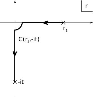
Figure 2: Contour of integration for conformal coordinates.

Note that as $t\rightarrow 0$, since $f(r)\rightarrow r$ as $r\rightarrow 0$, when $t\rightarrow 0$,

$$X(t)\sim\ln(-it)=\ln t-i\pi/2\,.$$ (23)

Now $f(-it)=-i\tilde{f}(t)$ for some real function $\tilde{f}$. Hence we find that

$$X(-it)=T(t)-i\pi/2$$ (24)

for some real function $T$. We define this function to be the conformal time coordinate. One finds that for

$$\tilde{a}(T(t))\equiv\tilde{f}(t)=if(-it)=ia(X(-it))=ia(T-i\pi/2)\,,$$ (25)

the metric becomes

$$ds^{2}={\tilde{a}}(T)^{2}(-dT^{2}+d\mathcal{H}^{2})$$ (26)

where $d\mathcal{H}^{2}$ is the metric on the hyperbolic space $\mathcal{H}^{3}$.

Note that in the $X\rightarrow-\infty$ limit, $a(X)\rightarrow Le^{X}$ for a length scale $L$. In the $T\rightarrow-\infty$ limit ${\tilde{a}}(T)\rightarrow Le^{T}$ for the same $L$. The analytic continuation is done by joining the Euclidean instanton and the Lorentzian background at the “hip,” by gluing $T\rightarrow-\infty$ and $X\rightarrow-\infty$. We explicitly work this “patching” out for the thin-wall case at the beginning of section 5.

Now let us expand the fluctuation of ${\hat{\varphi}}$ around this solution. Defining

$${\hat{\varphi}}(X,{\Omega})=a(X)^{-1}\varphi(X,{\Omega})$$ (27)

we obtain

$${\cal L}=\int dXd{\Omega}_{3}\sqrt{g_{S^{3}}}\left({1\over 2}\varphi(-\partial_{X}^{2}+U(X)-\Box)\varphi+{1\over 6}W(X)\varphi^{3}\right)+\mathcal{O}(\varphi^{4})$$ (28)

where $g_{S^{3}}$ refers to the $S^{3}$ metric and $\Box$ is the Laplacian on $S^{3}$. $U$ and $W$ are given by

$$U(X) ={a^{\prime\prime}(X)\over a(X)}+a^{2}(X){\delta^{2}\mathcal{V}\over\delta{\hat{\varphi}}^{2}}|_{\phi=\phi_{0},{\hat{\varphi}}=0}$$ (29)

$$W(X) =a(X){\delta^{3}\mathcal{V}\over\delta{\hat{\varphi}}^{3}}|_{\phi=\phi_{0},{\hat{\varphi}}=0}$$ (30)

We refer to $U(X)$ as the “radial potential” throughout this paper.

Our aim is to obtain an expression for

$$\langle\varphi(X_{1},{\Omega}_{1})\varphi(X_{2},{\Omega}_{2})\varphi(X_{3},{\Omega}_{3})\rangle$$ (31)

and its analytic continuation to Lorentzian signature. The three-point function for ${\hat{\varphi}}$ can be recovered by multiplying factors of $a(X_{i})^{-1}$ to the correlator of $\varphi$.

Later on, we consider two examples of potentials $\mathcal{V}$. We first consider a potential for which ${\hat{\varphi}}$ is massless on one side of the wall at $X=X_{0}$ in the thin-wall limit of the instanton. For example, the potential

$$\mathcal{V}={1\over 2}{m^{2}\over(\phi_{+}-\phi_{-})^{2}}(\phi-\phi_{-})^{2}{\hat{\varphi}}^{2}+{1\over 6}\lambda{(\phi-\phi_{-})\over(\phi_{+}-\phi_{-})}{\hat{\varphi}}^{3}+\mathcal{O}({\hat{\varphi}}^{4})\,.$$ (32)

serves the purpose as $\phi=\phi_{-}$ on one side of the thin wall and $\phi=\phi_{+}$ on the other.

$$U(X) =\begin{cases}{a^{\prime\prime}(X)\over a(X)}&(X<X_{0})\\ {a^{\prime\prime}(X)\over a(X)}+m^{2}a(X)^{2}&(X>X_{0})\end{cases}$$ (33)

$$W(X) =\begin{cases}0&(X<X_{0})\\ \lambda a(X)&(X>X_{0})\end{cases}$$ (34)

We refer to a scalar with this potential as a “massless scalar” throughout the paper, for lack of a better term.

We also consider the case when $\mathcal{V}$ is independent of $\phi$, i.e.,

$$\mathcal{V}={1\over 2}m^{2}{\hat{\varphi}}^{2}+{1\over 6}\lambda{\hat{\varphi}}^{3}+\mathcal{O}(\varphi^{4})\,.$$ (35)

The scalar must be massive in order for ${\hat{\varphi}}=0$ to be a stable point. Then

$$U(X) ={a^{\prime\prime}(X)\over a(X)}+m^{2}a(X)^{2}$$ (36)

$$W(X) =\lambda a(X)$$ (37)

3 Correlators in Euclidean Signature

In this section, we compute the two-point and three-point correlators on the Euclidean CDL instanton. We review the computation of the two-point function in section 3.1 for a general CDL instanton, assuming only mild conditions on the properties of the radial potential

$$U(X)={a^{\prime\prime}(X)\over a(X)}+a^{2}(X){\delta^{2}\mathcal{V}\over\delta{\hat{\varphi}}^{2}}|_{\phi=\phi_{0},{\hat{\varphi}}=0}\,.$$ (38)

Using the two-point function, we write an expression for the three-point function in section 3.2.

3.1 The Two-Point Function

We write out the two-point function in a form convenient for our purposes in this section. A more detailed account of the calculation can be found in [9, 36, 37, 38, 39]. Many of the results on one-dimensional scattering used in this section can be found in [9, 41].

Let us consider the Schrödinger equation,

$$(-\partial_{X}^{2}+U(X))\Psi_{E}(X)=E\Psi_{E}(X)\,,$$ (39)

where $U$ is the radial potential, (38). By properties of $a(X)$, it is easy to verify that

$$U(X)\rightarrow 1\quad\text{for }X\rightarrow\pm\infty\,.$$ (40)

So there exist a continuum of states labelled by real number $k$ that satisfy

$$(-\partial_{X}^{2}+U(X))\Psi_{k}(X)=(k^{2}+1)\Psi_{k}(X)\,.$$ (41)

There are two different bases that we can organize such solutions into. We define $\Psi_{k}$ to be the solutions that behave asymptotically as

$$\Psi_{k} \rightarrow\begin{cases}e^{ikX}+\mathcal{R}(k)e^{-ikX}&(X\rightarrow-\infty)\\ \mathcal{T}(k)e^{ikX}&(X\rightarrow\infty)\end{cases}$$ (42)

Also, we define $\Phi_{k}$ to be the solutions that behave asymptotically as

$$\Phi_{k} \rightarrow\begin{cases}\mathcal{T}(k)e^{-ikX}&(X\rightarrow-\infty)\\ e^{-ikX}-{\mathcal{R}(-k)\mathcal{T}(k)\over\mathcal{T}(-k)}e^{ikX}&(X\rightarrow\infty)\end{cases}$$ (43)

We note that for real $k$

$$\Psi_{-k}=\Psi_{k}^{*},\quad\Phi_{-k}=\Phi_{k}^{*}\,,$$ (44)

and hence that

$$\mathcal{R}(k)^{*}=\mathcal{R}(-k),\quad\mathcal{T}(k)^{*}=\mathcal{T}(-k)\,.$$ (45)

The unitarity relation $|\mathcal{R}|^{2}+|\mathcal{T}|^{2}=1$ becomes

$$\mathcal{R}(k)\mathcal{R}(-k)+\mathcal{T}(k)\mathcal{T}(-k)=1\,.$$ (46)

Also the two bases are related by

$$\Psi_{k} ={1\over\mathcal{T}(-k)}\Phi_{-k}+{\mathcal{R}(k)\over\mathcal{T}(k)}\Phi_{k}$$ (47)

$$\Phi_{k} ={1\over\mathcal{T}(-k)}\Psi_{-k}-{\mathcal{R}(-k)\over\mathcal{T}(-k)}\Psi_{k}\,.$$ (48)

There also can be bound states of this potential. We already know that

$$U(X)\rightarrow 1\quad\text{for }X\rightarrow\pm\infty\,.$$ (49)

In addition to this, we assume that the following holds:

1. The poles of $\Phi_{k}$, $\Psi_{k}$ and $\mathcal{T}(k)$ with respect to $k$ in the upper-half of the complex $k$ plane coincide and are simple.

2. The number of such poles are finite.

3. All such poles $iz$ lie on the imaginary axis and correspond to unique bound states of energy $(1-z^{2})$.

4. $\Phi_{k}/\mathcal{T}(k)$ does not have a pole in the upper-half of the complex $k$ plane.

5. $U(X)$ approaches $1$ as $X\rightarrow-\infty$ “rapidly.”

We refer to these conditions as “regularity conditions” throughout this paper. We have defined the meaning of “rapid” in appendix A. For our purposes, it is enough to note that exponential tails—($U(X)\sim 1+Ae^{NX}$)—are “rapid” enough.

The second condition means that for each pole $iz$ of $\mathcal{T}$ in the upper-half of the complex $k$ plane, there exists a bound state

$$u_{iz}(X)\propto\mathop{\text{Res}}_{k=iz}\Psi_{k}\propto\mathop{\text{Res}}_{k=iz}\Phi_{k}$$ (50)

such that

$$(-\partial_{X}^{2}+U(X))u_{iz}(X)=(-z^{2}+1)u_{iz}(X)\,.$$ (51)

All bound states are non-degenerate and hence their wavefunctions are real up to overall phase. We can fix the phase to be $0$.

These assumptions all hold when the potential $U(X)$ becomes constant for $X<X_{B}$ for some $X_{B}$. In that case, all the poles of the reflection coefficient $\mathcal{R}$ and transmission coefficient $\mathcal{T}$ coincide in the upper-half of the $k$ plane. Also, all these poles lie on the imaginary axis and correspond to unique bound states. We have slightly generalized these restrictions in our case. Rather than restricting the analytic structure of the scattering coefficients, we have restricted the analytic structure of the eigenfunctions themselves. We believe that these assumptions are not very strong, as we expect $\Phi,\Psi$ and $\mathcal{T}$ of a “generic” $U(X)$ to obey this property. We note that poles of $\Phi_{k},\Psi_{k}$ and $\mathcal{T}_{k}$ in the lower-half plane are relatively uncontrollable in contrast to the poles in the upper-half plane.

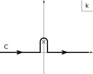
Figure 3: The contour $C$. $C$ runs along the real axis with a jump over the upmost pole of $\mathcal{T}$ marked by a cross.

Defining $C$ to be a contour in the complex $k$ plane that runs along the real axis with a jump over all the poles of $\mathcal{T}$ in the upper-half plane, the two-point function is given by [36, 37, 38]

$$\begin{split}G((X_{1},{\Omega}_{1}),(X_{2},{\Omega}_{2}))&\equiv\langle\varphi(X_{1},{\Omega}_{1})\varphi(X_{2},{\Omega}_{2})\rangle\\ &=\int_{C}{dk\over 2\pi}{\Phi_{k}(X)\Psi_{k}(X^{\prime})\over\mathcal{T}(k)}G_{k}({\Omega},{\Omega}^{\prime})\,.\end{split}$$ (52)

The contour $C$ is depicted in figure 3. $G_{k}$ is the propagator for a scalar

$$(\Box-(k^{2}+1))G_{k}({\Omega},{\Omega}^{\prime})={1\over\sqrt{g_{S^{3}}}}\delta({\Omega},{\Omega}^{\prime})\,.$$ (53)

Written out explicitly, it is [9]

$$G_{k_{i}}({\Omega},{\Omega}^{\prime})={\sinh k_{i}(\pi-{\Theta})\over\sinh k_{i}\pi\sin{\Theta}}\,.$$ (54)

${\Theta}({\Omega},{\Omega}^{\prime})$ is the angular distance from ${\Omega}$ to ${\Omega}^{\prime}$.

To show (57), we need to show that

$$\int_{C}{dk\over 2\pi}{\Phi_{k}(X)\Psi_{k}(X^{\prime})\over\mathcal{T}(k)}=\delta(X-X^{\prime})\,.$$ (55)

If this were true, then

$$\begin{split}&(-\partial_{X}^{2}+U(X)-\Box)\int_{C}{dk\over 2\pi}{\Phi_{-k}(X)\Psi_{k}(X^{\prime})\over\mathcal{T}(k)}G_{k}({\Omega},{\Omega}^{\prime})\\ &=\int_{C}{dk\over 2\pi}(-\partial_{X}^{2}+U(X)){\Phi_{-k}(X)\Psi_{k}(X^{\prime})\over\mathcal{T}(k)}G_{k}({\Omega},{\Omega}^{\prime})\\ &\qquad\qquad\qquad\qquad\qquad-\int_{C}{dk\over 2\pi}{\Phi_{-k}(X)\Psi_{k}(X^{\prime})\over\mathcal{T}(k)}\Box G_{k}({\Omega},{\Omega}^{\prime})\\ &=\int_{C}{dk\over 2\pi}{\Phi_{-k}(X)\Psi_{k}(X^{\prime})\over\mathcal{T}(k)}(k^{2}+1-\Box)G_{k}({\Omega},{\Omega}^{\prime})\\ &=\int_{C}{dk\over 2\pi}{\Phi_{-k}(X)\Psi_{k}(X^{\prime})\over\mathcal{T}(k)}{1\over\sqrt{g_{S^{3}}}}\delta({\Omega},{\Omega}^{\prime})\\ &={1\over\sqrt{g_{S^{3}}}}\delta(X-X^{\prime})\delta({\Omega},{\Omega}^{\prime})\end{split}$$ (56)

as desired. The completeness relation (55) is proven in appendix A.

To summarize, the two-point function on the Euclidean CDL instanton can be written in the form

$$\begin{split}\langle\varphi(X_{1},{\Omega}_{1})\varphi(X_{2},{\Omega}_{2})\rangle=\int_{C}{dk\over 2\pi}{\Phi_{k}(X)\Psi_{k}(X^{\prime})\over\mathcal{T}(k)}G_{k}({\Omega},{\Omega}^{\prime})\end{split}$$ (57)

when the potential $U(X)$ satisfies the regularity conditions. The contour of integration is defined to be a contour that runs along the real axis with a jump over the poles of $\mathcal{T}$; it is depicted in figure 3. We note once more that $U(X)\sim Ae^{NX}+1$ approaches $1$ in the limit $X\rightarrow-\infty$ rapidly enough to be regular.

3.2 The Three-Point Function

We find an expression for the tree-level three-point function

$$T({\{{X_{i}}\}},{\{{{\Omega}_{i}}\}})\equiv\langle\varphi(X_{1},{\Omega}_{1})\varphi(X_{2},{\Omega}_{2})\varphi(X_{3},{\Omega}_{3})\rangle$$ (58)

in this section. For notational simplicity, we use $\{x_{i}\}$ to denote the triplet $(x_{1},x_{2},x_{3})$ for any argument $x_{i}$ throughout the paper. Recall that the relevant part of the Lagrangian for computing the three-point function is

$${\cal L}=\int dXd{\Omega}_{3}\sqrt{g_{S^{3}}}\left({1\over 2}\varphi(-\partial_{X}^{2}+U(X)-\Box)\varphi+{1\over 6}W(X)\varphi^{3}\right)+\mathcal{O}(\varphi^{4})$$ (59)

and therefore

$$\begin{split}&T({\{{X_{i}}\}},{\{{{\Omega}_{i}}\}})\\ &=\int dXd{\Omega}W(X)G((X_{1},{\Omega}_{1}),(X,{\Omega}))G((X_{2},{\Omega}_{2}),(X,{\Omega}))G((X_{3},{\Omega}_{3}),(X,{\Omega}))\end{split}$$ (60)

at tree-level.

Using (57), we find that the full three-point function of $\varphi$ on the Euclidean instanton is given by

$$\begin{split}&T({\{{X_{i}}\}},{\{{{\Omega}_{i}}\}})\\ &=\int dXW(X)\int d{\Omega}\prod_{i}\left(\int_{C}{dk_{i}\over 2\pi}{\Phi_{k_{i}}(X_{i})\over\mathcal{T}(k_{i})}\Psi_{k_{i}}(X)G_{k_{i}}({\Omega},{\Omega}_{i})\right)\\ &=\left(\prod_{i}\int_{C}{dk_{i}\over 2\pi}{\Phi_{k_{i}}(X_{i})\over\mathcal{T}(k_{i})}\right)\left(\int dXW(X)\prod_{i}\Psi_{k_{i}}(X)\right)U_{\{{k_{i}}\}}({\{{{\Omega}_{i}}\}})\\ &=\left(\prod_{i}\int_{C}{dk_{i}\over 2\pi}{\Phi_{k_{i}}(X_{i})\over\mathcal{T}(k_{i})}\right)S({\{{k_{i}}\}})U_{\{{k_{i}}\}}({\{{{\Omega}_{i}}\}})\,.\end{split}$$ (61)

Here we have defined

$$S({\{{k_{i}}\}})=\int_{-\infty}^{\infty}dXW(X)\Psi_{k_{1}}(X)\Psi_{k_{2}}(X)\Psi_{k_{3}}(X)\,,$$ (62)

and

$$U_{k_{1},k_{2},k_{3}}({\Omega}_{1},{\Omega}_{2},{\Omega}_{3})\equiv\int d{\Omega}_{0}G_{k_{1}}({\Omega}_{1},{\Omega}_{0})G_{k_{2}}({\Omega}_{2},{\Omega}_{0})G_{k_{3}}({\Omega}_{3},{\Omega}_{0})\,.$$ (63)

As will be seen throughout this paper, $S({\{{k_{i}}\}})$ is the crucial data that determines the three-point function. We call $S$ the “wavefunction overlap.”

4 Analytic Continuation of the Three-Point Function

We analytically continue the Euclidean CDL three-point function to Lorentzian signature in this section and take various useful limits. As a first step, we analytically continue the three-point function on $S^{3}$ to $\mathcal{H}^{3}$ in section 4.1. Next, we use this result to write the holographic expansion of the CDL three-point function in section 4.2.

Lastly, we write the three-point function for points lying on the past lightcone of the FRW region in section 4.3. Recall that the past lightcone is at

$$T\rightarrow-\infty,\quad R\rightarrow\infty,\quad T+R=\text{(constant)}\,$$ (64)

as seen in the introduction. We expand the correlators in terms of $S^{2}$ harmonics.

4.1 Analytic Continuation of the Three-point Function on $S^{3}$

We first must understand how to analytically continue the three-point function on $S^{3}$ of three scalars $\phi_{1},\phi_{2},\phi_{3}$ that satisfy

$$(\Box-(k_{i}^{2}+1))\phi_{i}=0$$ (65)

with the interaction term

$$\phi_{1}\phi_{2}\phi_{3}\,.$$ (66)

We use the coordinates $(\theta,\phi,\varphi)$ on $S^{3}$ where ${\theta}$ and $\phi$ vary from $0$ to $\pi$ and the range of $\varphi$ is given by $[0,2\pi)$. The metric on $S^{3}$ is given by

$$ds^{2}=d\theta^{2}+\sin^{2}\theta d\omega^{2}\equiv d\theta^{2}+\sin^{2}\theta(d\phi^{2}+\sin^{2}\phi d\varphi^{2})\,.$$ (67)

We use ${\Omega}$ as shorthand for the $S^{3}$ coordinates $(\theta,\phi,\varphi)$ and $\omega$ as shorthand for the $S^{2}$ coordinates $(\phi,\varphi)$. The propagator for each scalar satisfying

$$(\Box-(k_{i}^{2}+1))G_{k_{i}}({\Omega},{\Omega}^{\prime})={1\over\sqrt{g_{S^{3}}}}\delta({\Omega},{\Omega}^{\prime})$$ (68)

is given by [9]

$$G_{k_{i}}({\Omega},{\Omega}^{\prime})={\sinh k_{i}(\pi-{\Theta})\over\sinh k_{i}\pi\sin{\Theta}}\,.$$ (69)

${\Theta}({\Omega},{\Omega}^{\prime})$ is the angular distance from ${\Omega}$ to ${\Omega}^{\prime}$;

$$\cos{\Theta}({\Omega},{\Omega}^{\prime})=\cos{\theta}\cos{\theta}^{\prime}+\sin{\theta}\sin{\theta}^{\prime}\cos\alpha(\omega,\omega^{\prime})\,.$$ (70)

Here $\alpha$ is the angular distance between the $S^{2}$ coordinates;

$$\cos\alpha(\omega,\omega^{\prime})=\cos\phi\cos\phi^{\prime}+\sin\phi\sin\phi^{\prime}\cos(\varphi-\varphi^{\prime})\,.$$ (71)

The three-point function is given by

$$U_{k_{1},k_{2},k_{3}}({\Omega}_{1},{\Omega}_{2},{\Omega}_{3})=\int d{\Omega}_{0}G_{k_{1}}({\Omega}_{1},{\Omega}_{0})G_{k_{2}}({\Omega}_{2},{\Omega}_{0})G_{k_{3}}({\Omega}_{3},{\Omega}_{0})\,,$$ (72)

which we have encountered at the end of section 3.2. Using the shorthand notation

$${\Theta}_{ij}={\Theta}({\Omega}_{i},{\Omega}_{j})\,,$$ (73)

this can be written as

$$U_{k_{1},k_{2},k_{3}}({\Omega}_{1},{\Omega}_{2},{\Omega}_{3})=\int_{0}^{\pi}d\theta_{0}\sin^{2}{\theta}_{0}\int d\omega_{0}\prod_{i}{\sinh k_{1}(\pi-{\Theta}_{i0})\over\sinh(k_{i}\pi)\sin{\Theta}_{i0}}\,.$$ (74)

As before, using the notation $\{x_{i}\}$ to denote the triplet $(x_{1},x_{2},x_{3})$ for any argument $x_{i}$, $U$ can be conveniently written as

$$U_{{\{{k_{i}}\}}}({\{{{\Omega}_{i}}\}})=U_{k_{1},k_{2},k_{3}}({\Omega}_{1},{\Omega}_{2},{\Omega}_{3})\,.$$ (75)

Let us analytically continue ${\theta}$ to $iR$. Then

$$-ds^{2}=dR^{2}+\sinh^{2}Rd\omega^{2}$$ (76)

is precisely the metric on hyperbolic space $\mathcal{H}^{3}$. Interpreting the coordinates $(R,\phi,\varphi)$ as coordinates on $\mathcal{H}^{3}$ we may analytically continue the arguments of $T$ to obtain a function on $\mathcal{H}^{3}$;

$$u_{\{{k_{i}}\}}({\{{(R_{i},\phi_{i},\varphi_{i})}\}})\equiv U_{\{{k_{i}}\}}({\{{(iR_{i},\phi_{i},\varphi_{i})}\}})\,.$$ (77)

We use $\mathcal{H}$ to denote the coordinates $(R,\phi,\varphi)$.

Now we deform the initial contour of integration $C$ for ${\theta}_{0}$ on the complex plane. The only potential poles are at ${\theta}=iR_{i}+n\pi$ for integer $n$ so we deform the contour of integration as in figure 4 and take $M$ to infinity. The new contour of integration can be broken in to 3 pieces $C_{1}$, $C_{2}$ and $C_{3}$, i.e.,

$$u_{\{{k_{i}}\}}({\{{\mathcal{H}_{i}}\}})=u^{1}_{\{{k_{i}}\}}({\{{\mathcal{H}_{i}}\}})+u^{2}_{\{{k_{i}}\}}({\{{\mathcal{H}_{i}}\}})+u^{3}_{\{{k_{i}}\}}({\{{\mathcal{H}_{i}}\}})\,,$$ (78)

where

$$u^{I}_{\{{k_{i}}\}}({\{{\mathcal{H}_{i}}\}})=\int_{C_{I}}d\theta_{0}\sin^{2}{\theta}_{0}\int d\omega_{0}\prod_{i}{\sinh k_{1}(\pi-{\Theta}_{i0})\over\sinh(k_{i}\pi)\sin{\Theta}_{i0}}\,.$$ (79)

Figure 4: Contour of integration for $\theta_{0}$.

As we take $M$ to infinity the integral over $C_{2}$ vanishes. This is because when ${\Omega}_{0}=(iM+{\theta}_{0},\phi_{0},\varphi_{0})$

$$\begin{split}&\cos{\Theta}_{i0}\\ &={1\over 2}e^{M}(\cos{\theta}_{0}(\cosh R_{i}+\sinh R_{i}\cos\alpha_{0i})+i\sin{\theta}_{0}(\cosh R_{i}-\sinh R_{i}\cos\alpha_{0i}))+\mathcal{O}(e^{-M})\\ &={1\over 2}e^{(M+\mathcal{O}(1))}(\cos{\theta}+i\sin{\theta})+\mathcal{O}(e^{-M})\,,\end{split}$$ (80)

where

$$\cot{\theta}=\left({\coth R_{i}+\cos\alpha_{0i}\over\coth R_{i}-\cos\alpha_{0i}}\right)\cot{\theta}_{0}\,.$$ (81)

Hence

$${\text{arccot}}(e^{2R_{i}}\cot{\theta}_{0})\leq{\theta}\leq{\text{arccot}}(e^{-2R_{i}}\cot{\theta}_{0})\,.$$ (82)

It is clear that ${\theta}$ slides from $0$ to $\pi$ as ${\theta}_{0}$ runs from $0$ to $\pi$. Since

$$\cos(-iM+\theta)={1\over 2}e^{(M+\mathcal{O}(1))}(\cos{\theta}+i\sin{\theta})+\mathcal{O}(e^{-M})$$ (83)

for large $M$, it is clear that up to corrections small in the limit of large $M$,

$${\Theta}_{i0}=-iM+\theta$$ (84)

where $\theta$ ranges from $0$ to $\pi$. Therefore

$$|\sin{\Theta}_{i0}|\simeq{1\over 2}e^{M}$$ (85)

for large $M$ and

$$\left|\sinh k_{i}(\pi-{\Theta}_{i0})\right|$$ (86)

is bounded above for given $\mathcal{H}_{1},\mathcal{H}_{2}$ and $\mathcal{H}_{3}$ for ${\theta}_{0}$ on $C_{2}$ since the real part of ${\Theta}_{i0}$ has finite range. Therefore

$$\left|\int_{C_{2}}d\theta_{0}\sin^{2}{\theta}_{0}\int d\omega_{0}\prod_{i}{\sinh k_{1}(\pi-{\Theta}_{i0})\over\sinh(k_{i}\pi)\sin{\Theta}_{i0}}\right|\sim\mathcal{O}(e^{-M})$$ (87)

and hence $u^{2}_{\{{k_{i}}\}}({\{{\mathcal{H}_{i}}\}})$ vanishes as $M\rightarrow\infty$.

Now let us carry out the integral along the contours $C_{1}$ and $C_{3}$.

$$\begin{split}\cos{\Theta}((iR,\omega),(iR^{\prime},\omega^{\prime}))&=\cosh R\cosh R^{\prime}-\sinh R\sinh R^{\prime}\cos\alpha(\omega,\omega^{\prime})\\ &=\cosh\ell(\mathcal{H},\mathcal{H}^{\prime})\end{split}$$ (88)

where $\ell(\mathcal{H},\mathcal{H}^{\prime})$ is the angular distance between two points in hyperbolic space. Therefore

$$\begin{split}G_{k_{j}}((iR_{0},\omega_{0}),(iR_{j},\omega_{j}))&={\sinh k_{j}(\pi-i\ell_{j0})\over\sinh(k_{j}\pi)\sin i\ell_{j0}}\\ &={e^{k_{j}\pi}e^{-ik_{j}\ell_{j0}}-e^{-k_{j}\pi}e^{ik_{j}\ell_{j0}}\over 2i\sinh(k_{j}\pi)\sinh\ell_{j0}}\,,\end{split}$$ (89)

when we take $\theta_{0}=iR$. We have defined

$$\ell_{ij}\equiv\ell(\mathcal{H}_{i},\mathcal{H}_{j})\,.$$ (90)

We can define the two-point function on $\mathcal{H}^{3}$ as

$$\mathcal{G}_{k}(\mathcal{H},\mathcal{H}^{\prime})={e^{ik\ell(\mathcal{H},\mathcal{H}^{\prime})}\over\sinh\ell(\mathcal{H},\mathcal{H}^{\prime})}\,.$$ (91)

Unlike in the case of $S^{3}$ there are two distinct solutions to

$$(\Box+k_{i}^{2})G_{k_{i}}(\mathcal{H},\mathcal{H}^{\prime})={1\over\sqrt{g_{\mathcal{H}^{3}}}}\delta(\mathcal{H},\mathcal{H}^{\prime})\,.$$ (92)

In (91), we have chosen a propagator that has “definite asymptotic behavior,” i.e.,

$$\mathcal{G}_{k}(\ell)\sim e^{(-1+ik)\ell}$$ (93)

for large $\ell$. With this definition we may write

$$\begin{split}G_{k_{j}}((iR_{0},\omega_{0}),(iR_{j},\omega_{j}))={e^{k_{j}\pi}\mathcal{G}_{-k_{j}}(\ell_{j0})-e^{-k_{j}\pi}\mathcal{G}_{k_{j}}(\ell_{j0})\over 2i\sinh(k_{j}\pi)}\,.\end{split}$$ (94)

Therefore

$$\begin{split}&u^{1}_{\{{k_{i}}\}}({\{{\mathcal{H}_{i}}\}})\\ &={1\over 8\prod_{i}\sinh k_{i}\pi}\sum_{\text{signs}}(\mp 1)(\mp 1)(\mp 1)e^{(\mp k_{1}\mp k_{2}\mp k_{3})\pi}\int_{0}^{\infty}dR_{0}\sinh^{2}R_{0}\int d\omega_{0}\prod_{i}\mathcal{G}_{\pm k_{i}}(\ell_{i0})\\ &={1\over 8\prod_{i}\sinh k_{i}\pi}\sum_{\text{signs}}(\mp 1)(\mp 1)(\mp 1)e^{(\mp k_{1}\mp k_{2}\mp k_{3})\pi}\int d\mathcal{H}_{0}\prod_{i}\mathcal{G}_{\pm k_{i}}(\mathcal{H}_{0},\mathcal{H}_{i})\,,\end{split}$$ (95)

where the sum are taken over the 8 combinations of assignments of signs. We can improve the notation by writing

$$\begin{split}&u^{1}_{\{{k_{i}}\}}({\{{\mathcal{H}_{i}}\}})\\ &={1\over 8\prod_{i}\sinh k_{i}\pi}\sum_{{\{{{\sigma}_{i}}\}}}(-{\sigma}_{1})(-{\sigma}_{2})(-{\sigma}_{3})e^{(-{\sigma}_{1}k_{1}-{\sigma}_{2}k_{2}-{\sigma}_{3}k_{3})\pi}\int_{0}^{\infty}dR_{0}\sinh^{2}R_{0}\int d\omega_{0}\prod_{i}\mathcal{G}_{{\sigma}_{i}k_{i}}(\ell_{i0})\\ &=-{1\over 8\prod_{i}\sinh k_{i}\pi}\sum_{{\{{{\sigma}_{i}}\}}}{\sigma}_{1}{\sigma}_{2}{\sigma}_{3}e^{-(\sum_{i}{\sigma}_{i}k_{i})\pi}\int d\mathcal{H}_{0}\prod_{i}\mathcal{G}_{{\sigma}_{i}k_{i}}(\mathcal{H}_{0},\mathcal{H}_{i})\,,\end{split}$$ (96)

where each ${\sigma}_{i}$ runs over the two values $(+1)$ and $(-1)$.

Meanwhile

$$\mathcal{U}_{\{{k_{i}}\}}({\{{\mathcal{H}_{i}}\}})=\int d\mathcal{H}_{0}\prod_{i}\mathcal{G}_{k_{i}}(\mathcal{H}_{0},\mathcal{H}_{i})$$ (97)

is precisely the three-point function on $\mathcal{H}^{3}$. At large values of $R_{1}=R_{2}=R_{3}=R$, $\mathcal{U}$ behaves as

$$\mathcal{U}_{\{{k_{i}}\}}({\{{\mathcal{H}_{i}}\}})\sim\mathcal{O}(e^{-3R+i(k_{1}+k_{2}+k_{3})R})\,.$$ (98)

Then

$$u^{1}_{\{{k_{i}}\}}({\{{\mathcal{H}_{i}}\}})=-{1\over 8\prod_{i}\sinh k_{i}\pi}\sum_{{\{{{\sigma}_{i}}\}}}{\sigma}_{1}{\sigma}_{2}{\sigma}_{3}e^{-(\sum_{i}{\sigma}_{i}k_{i})\pi}\mathcal{U}_{\{{{\sigma}_{i}k_{i}}\}}({\{{\mathcal{H}_{i}}\}})\,.$$ (99)

Likewise we can do the contour integration along $C_{3}$ by setting $\theta_{0}=iR_{0}+\pi$. Using

$$\begin{split}\cos{\Theta}((iR+\pi,\omega),(iR^{\prime},\omega^{\prime}))=\cosh(\ell(\mathcal{H},\mathcal{H}^{\prime})-i\pi)\,,\end{split}$$ (100)

we find that

$$\begin{split}G_{k_{j}}((iR_{0},\omega_{0}),(iR_{j},\omega_{j}))={-\mathcal{G}_{-k_{j}}(\ell_{j0})+\mathcal{G}_{k_{j}}(\ell_{j0})\over 2i\sinh(k_{j}\pi)}\end{split}$$ (101)

and

$$\begin{split}&u^{3}_{\{{k_{i}}\}}({\{{\mathcal{H}_{i}}\}})\\ &={1\over 8\prod_{i}\sinh k_{i}\pi}\sum_{{\{{{\sigma}_{i}}\}}}{\sigma}_{1}{\sigma}_{2}{\sigma}_{3}\int_{\infty}^{0}dR_{0}\sinh^{2}R_{0}\int d\omega_{0}\prod_{i}\mathcal{G}_{{\sigma}_{i}k_{i}}(\ell_{i0})\\ &=-{1\over 8\prod_{i}\sinh k_{i}\pi}\sum_{{\{{{\sigma}_{i}}\}}}{\sigma}_{1}{\sigma}_{2}{\sigma}_{3}\int d\mathcal{H}_{0}\prod_{i}\mathcal{G}_{{\sigma}_{i}k_{i}}(\mathcal{H}_{0},\mathcal{H}_{i})\,.\end{split}$$ (102)

Adding all the contributions up, the analytic continuation of $U$ becomes

$$u_{\{{k_{i}}\}}({\{{\mathcal{H}_{i}}\}})=-{1\over 8\prod_{i}\sinh k_{i}\pi}\sum_{{\{{{\sigma}_{i}}\}}}{\sigma}_{1}{\sigma}_{2}{\sigma}_{3}(1+e^{-(\sum_{i}{\sigma}_{i}k_{i})\pi})\mathcal{U}_{\{{{\sigma}_{i}k_{i}}\}}({\{{\mathcal{H}_{i}}\}})\,.$$ (103)

It is useful to write $\mathcal{U}_{\{{k_{i}}\}}$—the three-point function on $\mathcal{H}^{3}$—in Poincaré coordinates. Taking the $\mathcal{H}^{3}$ coordinates to be $(z,\vec{x})$ where $\vec{x}=(x_{1},x_{2})$ and the metric is given by

$$ds^{2}={dz^{2}+d\vec{x}^{2}\over z^{2}}\,,$$ (104)

the two-point correlator satisfies

$$\mathcal{G}_{k}(z,\vec{x};z^{\prime},\vec{x}^{\prime})=z^{(1-ik)}\left[{K_{\Delta=1-ik}(\vec{x};z^{\prime},\vec{x}^{\prime})\over-2ik}\right]$$ (105)

as $z\rightarrow 0$ [42]. Using the results of [43], we find that the three-point correlator

$$\begin{split}\mathcal{U}_{\{{k_{i}}\}}({\{{\mathcal{H}_{i}=(z_{i},\vec{x}_{i})}\}})=\int{dzd^{2}\vec{x}\over z^{3}}\prod_{i}\mathcal{G}_{k_{i}}(z_{i},\vec{x}_{i};z,\vec{x})\end{split}$$ (106)

in the $z_{i}\rightarrow 0$ limit goes to

$$\begin{split}&\mathcal{U}_{\{{k_{i}}\}}({\{{\mathcal{H}_{i}=(z_{i},\vec{x}_{i})}\}})\\ &\rightarrow{z_{1}^{(1-ik_{1})}z_{2}^{(1-ik_{2})}z_{3}^{(1-ik_{3})}\over 16\pi^{2}}{{\Gamma}({\Delta_{12}\over 2}){\Gamma}({\Delta_{23}\over 2}){\Gamma}({\Delta_{31}\over 2}){\Gamma}({1\over 2}(\Delta_{1}+\Delta_{2}+\Delta_{3}-2))\over{\Gamma}(\Delta_{1}){\Gamma}(\Delta_{2}){\Gamma}(\Delta_{3})}\\ &\times{1\over|x_{12}|^{\Delta_{12}}|x_{23}|^{\Delta_{23}}|x_{31}|^{\Delta_{31}}}\end{split}$$ (107)

where $\Delta_{l}=1-ik_{l}$, $|x_{lm}|=|\vec{x}_{l}-\vec{x}_{m}|$ and

$$\Delta_{lm}=\Delta_{l}+\Delta_{m}-\epsilon_{lmn}\Delta_{n}=1-ik_{l}-ik_{m}+i\epsilon_{lmn}k_{n}\,.$$ (108)

It proves convenient to denote

$$\tau_{\{{\Delta_{i}}\}}({\{{\vec{x}_{i}}\}})\equiv{1\over|x_{12}|^{\Delta_{12}}|x_{23}|^{\Delta_{23}}|x_{31}|^{\Delta_{31}}}$$ (109)

and

$$c_{\{{\Delta_{i}}\}}\equiv{{\Gamma}({\Delta_{12}\over 2}){\Gamma}({\Delta_{23}\over 2}){\Gamma}({\Delta_{31}\over 2}){\Gamma}({1\over 2}(\Delta_{1}+\Delta_{2}+\Delta_{3}-2))\over{\Gamma}(\Delta_{1}){\Gamma}(\Delta_{2}){\Gamma}(\Delta_{3})}\,.$$ (110)

4.2 The Holographic Series Expansion of the Full Three-point Function

Let us now analytically continue the full three-point function on the Euclidean instanton (61):

$$\begin{split}&T({\{{X_{i}}\}},{\{{{\Omega}_{i}}\}})\\ &=\int dXW(X)\int d{\Omega}\prod_{i}\left(\int_{C}{dk_{i}\over 2\pi}{\Phi_{k_{i}}(X_{i})\over\mathcal{T}(k_{i})}\Psi_{k_{i}}(X)G_{k_{i}}({\Omega},{\Omega}_{i})\right)\\ &=\left(\prod_{i}\int_{C}{dk_{i}\over 2\pi}{\Phi_{k_{i}}(X_{i})\over\mathcal{T}(k_{i})}\right)\left(\int dXW(X)\prod_{i}\Psi_{k_{i}}(X)\right)U_{\{{k_{i}}\}}({\{{{\Omega}_{i}}\}})\\ &=\left(\prod_{i}\int_{C}{dk_{i}\over 2\pi}{\Phi_{k_{i}}(X_{i})\over\mathcal{T}(k_{i})}\right)S({\{{k_{i}}\}})U_{\{{k_{i}}\}}({\{{{\Omega}_{i}}\}})\,.\end{split}$$ (111)

We are interested in the “near boundary limit” of the correlators. That is, we look at the behavior of the three-point function as we take the three points near the boundary of $\mathcal{H}^{3}$, i.e., we take $z_{i}\rightarrow 0$ in Poincaré coordinates.

We first analytically continue the spherical coordinates ${\Omega}_{j}$ to $\mathcal{H}_{j}$ by taking $\theta_{j}\rightarrow iR_{j}$. As elaborated in the previous section, $U_{\{{k_{i}}\}}({\{{{\Omega}_{i}}\}})$ analytically continues to $u_{\{{k_{i}}\}}({\{{{\Omega}_{i}}\}})$. By the discussion at the end of the last section we know that the near boundary limit of $u$ is given by

$$\begin{split}u_{\{{k_{i}}\}}({\{{\mathcal{H}_{i}}\}})&=-{1\over 8\prod_{i}\sinh k_{i}\pi}\sum_{{\{{{\sigma}_{i}}\}}}{\sigma}_{1}{\sigma}_{2}{\sigma}_{3}(1+e^{-(\sum_{i}{\sigma}_{i}k_{i})\pi})\mathcal{U}_{\{{{\sigma}_{i}k_{i}}\}}({\{{\mathcal{H}_{i}}\}})\\ &\rightarrow-{1\over 128\pi^{2}\prod_{i}\sinh k_{i}\pi}\sum_{{\{{{\sigma}_{i}}\}}}{\sigma}_{1}{\sigma}_{2}{\sigma}_{3}(1+e^{-(\sum_{i}{\sigma}_{i}k_{i})\pi})\\ &\times(\prod_{i}z^{1-i{\sigma}_{i}k_{i}})c_{\{{1-i{\sigma}_{i}k_{i}}\}}\tau_{\{{1-i{\sigma}_{i}k_{i}}\}}({\{{\vec{x}_{i}}\}})\,.\end{split}$$ (112)

Now defining

$${\hat{S}}_{\{{{\sigma}_{i}}\}}({\{{k_{i}}\}})\equiv{(1+e^{-(\sum_{i}{\sigma}_{i}k_{i})\pi})c_{\{{1-i{\sigma}_{i}k_{i}}\}}\over 128\pi^{2}\prod_{i}\sinh k_{i}\pi}S({\{{k_{i}}\}})$$ (113)

we find that in the near-boundary limit,

$$\begin{split}&T({\{{X_{i}}\}},{\{{\mathcal{H}_{i}}\}})\\ &=-\left(\prod_{i}\int_{C}{dk_{i}\over 2\pi}{\Phi_{k_{i}}(X_{i})\over\mathcal{T}(k_{i})}\right)\sum_{\{{{\sigma}_{i}}\}}{\sigma}_{1}{\sigma}_{2}{\sigma}_{3}{\hat{S}}_{\{{{\sigma}_{i}}\}}({\{{k_{i}}\}})(\prod_{i}z^{1-i{\sigma}_{i}k_{i}})\tau_{\{{1-i{\sigma}_{i}k_{i}}\}}({\{{\vec{x}_{i}}\}})\,\end{split}$$ (114)

as $z\rightarrow 0$.

In this limit, the $|k_{i}|\rightarrow\infty$ behavior is dictated by $z^{1\mp ik_{i}}$. That is, for terms of the integrand with $z$ dependence $z^{1-ik_{i}}$ we may deform the contour $C$ “upwards” towards $k_{i}\rightarrow i\infty$, while for terms with $z$ dependence $z^{1+ik_{i}}$ we can deform the contour $C$ “downwards” towards $k_{i}\rightarrow-i\infty$. More concisely, we may deform terms with $z$ dependence $z^{1-i{\sigma}_{i}k_{i}}$ towards $k_{i}\rightarrow i{\sigma}_{i}\infty$ when $z\rightarrow 0$. By deforming the terms in the integrand accordingly, the integral can be written as a sum of contributions from codimension-three poles of the integrand, i.e., poles of the form

$$E^{\{{\sigma_{i}}\}}_{\{{k_{i}}\}}({\{{X_{i}}\}})\equiv\left(\prod_{i}{\Phi_{k_{i}}\over\mathcal{T}(k_{i})}\right){\hat{S}}_{\{{{\sigma}_{i}}\}}({\{{k_{i}}\}})\sim{x\over(k_{1}-p_{1})(k_{2}-p_{2})(k_{3}-p_{3})}+\cdots$$ (115)

near ${\{{k_{i}}\}}={\{{p_{i}}\}}$.

Let us denote the $H_{i}^{(+1)}$ the upper-half of the complex $k_{i}$ plane divided by contour $C$ and $H_{i}^{(-1)}$ the lower-half. Let us also denote the codimension-three poles of ${\hat{S}}_{\{{{\sigma}_{i}}\}}({\{{k_{i}}\}})$ with respect to $k_{i}$ in $H_{1}^{{\sigma}_{1}}\times H_{2}^{{\sigma}_{2}}\times H_{3}^{{\sigma}_{3}}$ as $(i{\sigma}_{1}n_{r_{1}}^{{\sigma}_{1}},i{\sigma}_{2}n_{r_{2}}^{{\sigma}_{2}},i{\sigma}_{3}n_{r_{3}}^{{\sigma}_{3}})$, or in short, ${\{{i{\sigma}_{i}n_{r_{i}}^{{\sigma}_{i}}}\}}$. Then by doing the contour integral and picking up the poles of the integrand for each pole we obtain

$$\begin{split}&T({\{{X_{i}}\}},{\{{\mathcal{H}_{i}}\}})\\ &=-\left(\prod_{i}\int_{C}{dk_{i}\over 2\pi}{\Phi_{k_{i}}(X_{i})\over\mathcal{T}(k_{i})}\right)\sum_{\{{{\sigma}_{i}}\}}{\sigma}_{1}{\sigma}_{2}{\sigma}_{3}{\hat{S}}_{\{{{\sigma}_{i}}\}}({\{{k_{i}}\}})(\prod_{i}z^{1-i{\sigma}_{i}k_{i}})\tau_{\{{1-i{\sigma}_{i}k_{i}}\}}({\{{\vec{x}_{i}}\}})\\ &=i\sum_{\{{{\sigma}_{i}}\}}\sum_{\{{n_{r_{i}}^{{\sigma}_{i}}}\}}\hat{F}^{\{{{\sigma}_{i}}\}}_{\{{n^{{\sigma}_{i}}_{r_{i}}}\}}({\{{X_{i}}\}})(\prod_{i}z^{n^{{\sigma}_{i}}_{r_{i}}+1})\tau_{\{{n^{{\sigma}_{i}}_{r_{i}}+1}\}}({\{{\vec{x}_{i}}\}})\\ &\quad+\text{(Double Pole Contributions)}\end{split}$$ (116)

where we have defined

$$\hat{F}^{\{{{\sigma}_{i}}\}}_{\{{n^{{\sigma}_{i}}_{r_{i}}}\}}({\{{X_{i}}\}})=\mathop{\text{Res}}_{{\{{k_{i}}\}}={\{{i{\sigma}_{i}n^{{\sigma}_{i}}_{r_{i}}}\}}}E^{\{{\sigma_{i}}\}}_{\{{k_{i}}\}}({\{{X_{i}}\}})\,.$$ (117)

As indicated in the equation there may be additional terms coming from the double poles of $E^{\{{\sigma_{i}}\}}_{\{{k_{i}}\}}({\{{X_{i}}\}})$ with respect to $k_{i}$, which certainly exist in general.

Finally we analytically continue $X_{i}$ to obtain the holographic expansion of the three-point function:

$$\begin{split}&\langle{\hat{\varphi}}(T_{1},\mathcal{H}_{1}){\hat{\varphi}}(T_{2},\mathcal{H}_{2}){\hat{\varphi}}(T_{3},\mathcal{H}_{3})\rangle\\ &=\left[\prod_{i}a(T_{i}-i\pi/2)^{-1}\right]T({\{{T_{i}-i\pi/2}\}},{\{{\mathcal{H}_{i}}\}})\\ &=(-i)\left[\prod_{i}{\tilde{a}}(T_{i})^{-1}\right]T({\{{T_{i}-i\pi/2}\}},{\{{\mathcal{H}_{i}}\}})\\ &=\sum_{\{{{\sigma}_{i}}\}}\sum_{\{{n_{r_{i}}^{{\sigma}_{i}}}\}}F^{\{{{\sigma}_{i}}\}}_{\{{n^{{\sigma}_{i}}_{r_{i}}+1}\}}({\{{T_{i}}\}})(\prod_{i}z^{n^{{\sigma}_{i}}_{r_{i}}+1})\tau_{\{{n^{{\sigma}_{i}}_{r_{i}}+1}\}}({\{{\vec{x}_{i}}\}})\\ &\qquad+\text{(Double Pole Contributions)}\end{split}$$ (118)

$F^{\{{{\sigma}_{i}}\}}_{\{{n^{{\sigma}_{i}}_{r_{i}}+1}\}}({\{{T_{i}}\}})$ is defined as

$$F^{\{{{\sigma}_{i}}\}}_{\{{n^{{\sigma}_{i}}_{r_{i}}+1}\}}({\{{T_{i}}\}})\equiv\left[\prod_{i}{\tilde{a}}(T_{i})^{-1}\right]\mathop{\text{Res}}_{{\{{k_{i}}\}}={\{{i{\sigma}_{i}n^{{\sigma}_{i}}_{r_{i}}}\}}}E^{\{{\sigma_{i}}\}}_{\{{k_{i}}\}}({\{{T_{i}-i\pi/2}\}})\,.$$ (119)

Now let us examine the behavior of $F^{\{{{\sigma}_{i}}\}}_{\{{n_{i}+1}\}}({\{{T_{i}}\}})$ at early times. $\Phi_{k}/\mathcal{T}(k)$ has exponential $T$ scaling at early times. More precisely, $\Phi_{k}(X)/\mathcal{T}(k)$ can be written as

$${\Phi_{k}(X)\over\mathcal{T}(k)}=e^{-ikX}\left(1+\sum_{n=1}^{\infty}c_{n}(k)e^{nX}\right)$$ (120)

near $X\rightarrow-\infty$. $c_{n}$ may have poles in $k$. From the definition of $E^{\{{\sigma_{i}}\}}_{\{{k_{i}}\}}({\{{X_{i}}\}})$ it can be shown that in the early-time limit

$$\begin{split}&\left[\prod_{i}{\tilde{a}}(T_{i})^{-1}\right]E^{\{{\sigma_{i}}\}}_{\{{k_{i}}\}}({\{{T_{i}-i\pi/2}\}})\\ &=\left(\prod_{i}{\Phi_{k_{i}}(T_{i}-i\pi/2)\over{\tilde{a}}(T_{i})\mathcal{T}(k_{i})}\right){\hat{S}}_{\{{{\sigma}_{i}}\}}({\{{k_{i}}\}})\\ &\rightarrow\left({1\over L^{3}}\right){\hat{S}}_{\{{{\sigma}_{i}}\}}({\{{k_{i}}\}})e^{-\sum_{i}k_{i}\pi/2}e^{\sum_{i}(-1-ik_{i})T_{i}}\,.\end{split}$$ (121)

The terms in (118) relevant in the early-time limit $T_{i}\rightarrow-\infty$ are given by poles of ${\hat{S}}_{\{{{\sigma}_{i}}\}}({\{{k_{i}}\}})$ when ${\{{{\sigma}_{i}}\}}=(-1,-1,-1)$—they come from picking up poles of the integrand that are in the lower-half $k$ plane. The terms of the holographic expansion coming from these poles are proportional to

$$(\prod_{i}e^{-\Delta_{i}T_{i}}z^{\Delta_{i}})\tau_{\{{\Delta_{i}}\}}({\{{\vec{x}_{i}}\}})$$ (122)

for $\Delta_{i}=n^{-}_{r_{i}}+1$, as promised in the introduction.

In general, terms in the expansion that come from double poles have factors of $(\ln T)$, $(\ln z)$ or $(\ln|x_{ij}|)$ multiplied to the “conformal” form (122) in the early-time limit. It can be seen, however, that any double pole coming from poles of $\Phi_{k}/\mathcal{T}(k)$ are due to poles of $c_{n}$. Hence double pole contributions of this kind are always subleading in $e^{T}$ in the early-time limit and can be ignored.

To write out all the terms of the early-time holographic expansion, one must locate all the poles of the integrand carefully and compute its residues and take the early-time limit. There are many terms that have to be computed on a case-by-case basis that depend on the structure of $\Phi_{k}/\mathcal{T}(k)$ and $S({\{{k_{i}}\}})$. Most of the terms, however, are “universal” in any early-time holographic expansion. These terms come from picking up “generic poles” at ${\{{-in^{-}_{r_{i}}}\}}\in H^{-1}_{k_{1}}\times H^{-1}_{k_{2}}\times H^{-1}_{k_{3}}$. We define “generic poles” ${\{{i{\sigma}_{i}n^{{\sigma}_{i}}_{r_{i}}}\}}\in H^{{\sigma}_{1}}_{k_{1}}\times H^{{\sigma}_{2}}_{k_{2}}\times H^{{\sigma}_{3}}_{k_{3}}$ to be points that satisfy the following conditions:

1. $n^{{\sigma}_{i}}_{r_{i}}$ are integers.

2. The triplet ${\{{n^{{\sigma}_{i}}_{r_{i}}+1}\}}$ satisfies the triangle inequality.

3. ${\{{k_{i}}\}}={\{{i{\sigma}_{i}n^{{\sigma}_{i}}_{r_{i}}}\}}$ is either

   1. not a pole of $S({\{{k_{i}}\}})$,

   2. or lies on a codimension-one pole of $S({\{{k_{i}}\}})$ and $\sum_{i}n^{{\sigma}_{i}}_{r_{i}}$ is odd.

The contribution of a generic pole ${\{{k_{i}}\}}={\{{-in^{-}_{r_{i}}}\}}$ to the early-time three-point function is

$$\begin{split}&\rightarrow\left({i\over 64\pi^{5}L^{3}}\right)e^{-i\pi(\sum_{i}\Delta^{-}_{r_{i}})/2}\sin\left({\pi\sum_{i}\Delta^{-}_{r_{i}}\over 2}\right){S({\{{-i(\Delta_{r_{i}}^{-}-1)}\}})}c_{\{{\Delta^{-}_{r_{i}}}\}}\\ &\qquad\times(\prod_{i}e^{-\Delta^{-}_{r_{i}}T_{i}}z^{\Delta^{-}_{r_{i}}})\tau_{\{{\Delta^{-}_{r_{i}}}\}}({\{{\vec{x}_{i}}\}})\end{split}$$ (123)

where we have defined $\Delta^{{\sigma}}_{r}=n^{{\sigma}}_{r}+1$.

We note that contrary to the early-time limit $T_{i}\rightarrow-\infty$, we cannot obtain the late time limit $T_{i}\rightarrow\infty$ of $\Phi_{k}$ by plugging in $X\rightarrow T-i\pi/2$ to the $X\rightarrow\infty$ limit of $\Phi_{k}$ in (43). This is because we are “gluing” the modes on the Euclidean instanton and the cosmological background at $r=0$, where $r$ is the radial coordinate of the instanton. This is equivalent to gluing the modes at $X,T\rightarrow-\infty$ with respect to the conformal coordinates $X$ and $T$.

4.3 Spherical Harmonics expansion of the Three-Point function
on the Past Lightcone

Let us expand the three-point function in terms of $S^{2}$ harmonics when the points lie on the past lightcone of the FRW region, i.e., when

$$T_{1},T_{2},T_{3} \rightarrow-\infty$$ (124)

$$R_{1},R_{2},R_{3} \rightarrow\infty$$ (125)

$$T_{i}+R_{i} :\text{(finite)}$$ (126)

To do so, let us go back to expression (61) and analytically continue the $S^{3}$ coordinates to $\mathcal{H}^{3}$ coordinates:

$$\begin{split}&T({\{{X_{i}}\}},{\{{\mathcal{H}_{i}}\}})\\ &=-\left(\prod_{i}\int_{C}{dk_{i}\over 4\pi\sinh k_{i}\pi}{\Phi_{k_{i}}(X_{i})\over\mathcal{T}(k_{i})}\right)S({\{{k_{i}}\}})\\ &\quad\times\sum_{\{{{\sigma}_{i}}\}}{\sigma}_{1}{\sigma}_{2}{\sigma}_{3}(1+e^{-(\sum_{i}{\sigma}_{i}k_{i})\pi})\mathcal{U}_{\{{{\sigma}_{i}k_{i}}\}}({\{{\mathcal{H}_{i}}\}})\,.\end{split}$$ (127)

Now let us write $\mathcal{U}_{\{{k_{i}}\}}$ in terms of harmonics. Recall that $\mathcal{U}_{\{{k_{i}}\}}$ is defined by

$$\mathcal{U}_{\{{k_{i}}\}}({\{{\mathcal{H}_{i}}\}})=\int d\mathcal{H}_{0}\prod_{i}\mathcal{G}_{k_{i}}(\mathcal{H}_{0},\mathcal{H}_{i})\,.$$ (128)

The correlators $\mathcal{G}_{k}(\mathcal{H}_{0},\mathcal{H})$ can be written in terms of scalar eigenmodes on $\mathcal{H}^{3}$ [44, 45]

$$q_{klm}(\mathcal{H})\equiv q_{kl}(R)Y_{lm}(\omega)\,,$$ (129)

where

$$\begin{split}q_{kl}(R)&=(i\sinh R)^{l}F(ik+l+1,-ik+l+1;l+{3\over 2};-\sinh^{2}{R\over 2})\\ &={2(-2i)^{l}{\Gamma}(l+3/2)\over\sqrt{\pi}k\prod_{j=1}^{l}(k^{2}+j^{2})}(\sinh R)^{l}({d\over d\cosh R})^{l}{\sin kR\over\sinh R}\,,\end{split}$$ (130)

and $Y_{lm}$ are the spherical harmonic functions.

Then

$$\mathcal{G}_{k}(\mathcal{H}_{0},\mathcal{H})={1\over 2}\sum_{l,m}\int_{C_{k}}dp{N_{l}(p)\over p^{2}-k^{2}}q_{pl(-m)}(\mathcal{H}_{0})q_{plm}(\mathcal{H})\,,$$ (131)

where $C_{k}$—depicted in figure 5—is the contour of integration. $N_{l}(p)$ is a normalization constant:

$$\begin{split}N_{l}(p)&={(-1)^{l}{\Gamma}(ip+l+1){\Gamma}(-ip+l+1)\over 2^{2l+1}{\Gamma}(l+{3\over 2})^{2}{\Gamma}(ip){\Gamma}(-ip)}={(-1)^{l}\prod_{j=0}^{l}(p^{2}+j^{2})\over 2^{2l+1}{\Gamma}(l+3/2)^{2}}\,.\end{split}$$ (132)

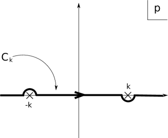
Figure 5: The contour $C_{k}$. The contour $C_{-k}$ follows from the definition of $C_{k}$.

Then $\mathcal{U}_{\{{k_{i}}\}}$ can be written as

$$\begin{split}&\mathcal{U}_{\{{k_{i}}\}}({\{{\mathcal{H}_{i}}\}})=\\ &{1\over 8}\sum_{l_{i},m_{i}}\left[\prod_{i}\left(\int_{C_{k_{i}}}{dp_{i}\over p_{i}^{2}-k_{i}^{2}}\right)\left(\prod_{i}q_{p_{i}l_{i}m_{i}}(\mathcal{H})\right)\int d\mathcal{H}_{0}\left(\prod_{i}{N_{l_{i}}(p_{i})q_{p_{i}l_{i}(-m_{i})}(\mathcal{H}_{0})}\right)\right]\,.\end{split}$$ (133)

We define

$$B({\{{p_{i},l_{i},m_{i}}\}})\equiv\int d\mathcal{H}_{0}\left(\prod_{i}{N_{l_{i}}(p_{i})q_{p_{i}l_{i}(-m_{i})}(\mathcal{H}_{0})}\right)$$ (134)

which can be thought of as structure functions on $\mathcal{H}^{3}$ similar to Wigner coefficients on $S^{2}$. We have listed some important properties of $B({\{{p_{i},l_{i},m_{i}}\}})$ in appendix B.

The analytically continued full three-point function may be rewritten as

$$\begin{split}&T({\{{X_{i}}\}},{\{{\mathcal{H}_{i}}\}})\\ &=-{1\over 64}\sum_{\{{{\sigma}_{i}}\}}\prod_{i}\left(\int_{-\infty}^{\infty}dp_{i}\right)\sum_{l_{i},m_{i}}B({\{{p_{i},l_{i},m_{i}}\}})\left(\prod_{i}q_{p_{i}l_{i}m_{i}}(\mathcal{H}_{i})\right)\\ &\quad\left(\prod_{i}\int_{C^{\prime}_{p_{i},{\sigma}_{i}}}{dk_{i}\Phi_{k_{i}}(X_{i})\over 2\pi\mathcal{T}(k_{i})\sinh k_{i}\pi(p_{i}^{2}-k_{i}^{2})}\right)S({\{{k_{i}}\}}){\sigma}_{1}{\sigma}_{2}{\sigma}_{3}(1+e^{-(\sum_{i}{\sigma}_{i}k_{i})\pi})\,.\end{split}$$ (135)

As we have switched the order of integration, the contour of integration of the $k_{i}$’s have been changed to $C^{\prime}_{p_{i},{\sigma}_{i}}$ which is depicted in figure 6.

In the $X\rightarrow(-\infty-i\pi/2)$ limit, or the $T\rightarrow-\infty$ limit, there is a useful expansion in terms of $e^{T}$. In this limit

$${\Phi_{k}(T-i\pi/2)\over\mathcal{T}(k)}\rightarrow e^{-ik(T-i\pi/2)}$$ (136)

Therefore all the contours of integration for $k_{i}$ can be deformed upward and the poles $k_{i}$ with $({\rm Im}~{}k_{i})>0$ and possibly $k_{i}=\pm p_{i}$ contribute. Hence

$$\begin{split}&-\sum_{\{{{\sigma}_{i}}\}}\left(\prod_{i}\int_{C^{\prime}_{p_{i},{\sigma}_{i}}}{dk_{i}e^{-ik_{i}(T_{i}-i\pi/2)}\over 2\pi\sinh k_{i}\pi(p_{i}^{2}-k_{i}^{2})}\right)S({\{{k_{i}}\}}){\sigma}_{1}{\sigma}_{2}{\sigma}_{3}(1+e^{-(\sum_{i}{\sigma}_{i}k_{i})\pi})\\ &={i\over 4\prod_{i}p_{i}\sinh\pi p_{i}}\sum_{\{{s_{i}}\}}S({\{{s_{i}p_{i}}\}})\cosh{\pi(\sum_{i}s_{i}p_{i})\over 2}e^{-i\sum_{i}s_{i}p_{i}T_{i}}\\ &+\sum_{{\{{{\sigma}_{i}}\}}\neq(-1,-1,-1)}\sum_{(\text{at least one }n_{i}>0)}\mathcal{O}(e^{\sum_{i}n_{i}T_{i}})\,.\end{split}$$ (137)

The leading term comes from the poles $\pm p_{i}$ that are picked up for the contour integral along $C_{k_{1},(-1)}\times C_{k_{2},(-1)}\times C_{k_{3},(-1)}$. Each $s_{i}$ is summed over $(+1)$ and $(-1)$. The subleading terms in $e^{T}$ come from other combinations of contours.

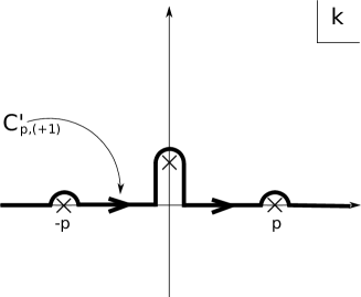
Figure 6: The contours $C^{\prime}_{p,(+1)}$ and $C^{\prime}_{p,(-1)}$. The cross on the imaginary axis is the upmost pole of $\mathcal{T}(k)$.

In the limit $T_{1},T_{2},T_{3}\rightarrow-\infty$ the integrand is equal to the leading term. Therefore on the past lightcone

$$\begin{split}&T({\{{T_{i}-i\pi/2}\}},{\{{\mathcal{H}_{i}}\}})\\ &={1\over 64}\prod_{i}\left(\int_{-\infty}^{\infty}dp_{i}\right)\sum_{l_{i},m_{i}}B({\{{p_{i},l_{i},m_{i}}\}})\left(\prod_{i}q_{p_{i}l_{i}m_{i}}(\mathcal{H}_{i})\right)\\ &\quad\times{i\over 4\prod_{i}p_{i}\sinh\pi p_{i}}\sum_{\{{s_{i}}\}}S({\{{s_{i}p_{i}}\}})\cosh{\pi(\sum_{i}s_{i}p_{i})\over 2}e^{-i\sum_{i}s_{i}p_{i}T_{i}}\,.\end{split}$$ (138)

$B({\{{p_{i},l_{i},m_{i}}\}})$, $q_{p_{i}l_{i}(-m_{i})}(\mathcal{H}_{i})$ and $p_{i}\sinh\pi p_{i}$ are all even with respect to $p_{i}$. Therefore we can rewrite the integral as

$$\begin{split}&T({\{{T_{i}-i\pi/2}\}},{\{{\mathcal{H}_{i}}\}})\\ &={i\over 32}\prod_{i}\left(\int_{-\infty}^{\infty}dp_{i}\right)\sum_{l_{i},m_{i}}B({\{{p_{i},l_{i},m_{i}}\}})\left(\prod_{i}q_{p_{i}l_{i}m_{i}}(\mathcal{H}_{i})\right)\\ &\quad\times{\cosh{\pi(p_{1}+p_{2}+p_{3})\over 2}\over\prod_{i}p_{i}\sinh\pi p_{i}}S({\{{-p_{i}}\}})e^{ip_{1}T_{1}}e^{ip_{2}T_{2}}e^{ip_{3}T_{3}}\end{split}$$ (139)

for points on the past lightcone. In appendix B we show that $B({\{{p_{i},l_{i},m_{i}}\}})$ has a zero of order two for each $p_{i}$ at $p_{i}=0$. Hence the integrand does not have any poles along the real line.

In the large $R$ limit, $q_{plm}(R,\omega)$ behaves as [44]

$$\begin{split}q_{plm}(R,\omega)&\sim(-i){(2i)^{l+1}{\Gamma}(l+{3\over 2}){\Gamma}(ip)\over\sqrt{\pi}{\Gamma}(ip+l+1)}e^{(-1+ip)R}Y_{lm}(\omega)\\ &+(-i){(2i)^{l+1}{\Gamma}(l+{3\over 2}){\Gamma}(-ip)\over\sqrt{\pi}{\Gamma}(-ip+l+1)}e^{(-1-ip)R}Y_{lm}(\omega)\,.\end{split}$$ (140)

Therefore on the past lightcone

$$\begin{split}&T({\{{T_{i}-i\pi/2}\}},{\{{\mathcal{H}_{i}}\}})\\ &=\sum_{\{{l_{i},m_{i}}\}}e^{-R_{1}-R_{2}-R_{3}}K_{\{{l_{i},m_{i}}\}}({\{{T_{i},R_{i}}\}})Y_{l_{1}m_{1}}(\omega_{1})Y_{l_{2}m_{2}}(\omega_{2})Y_{l_{3}m_{3}}(\omega_{3})\end{split}$$ (141)

where

$$\begin{split}&K_{\{{l_{i},m_{i}}\}}({\{{T_{i},R_{i}}\}})\\ &=-{1\over 32}\prod_{i}\left(\int_{-\infty}^{\infty}dp_{i}\right){B({\{{p_{i},l_{i},m_{i}}\}})\over\prod_{i}p_{i}\sinh\pi p_{i}}{S({\{{-p_{i}}\}})}\cosh{\pi(p_{1}+p_{2}+p_{3})\over 2}\\ &\quad\times\sum_{\{{{\sigma}_{i}}\}}\left(\prod_{i}{(2i)^{l_{i}+1}{\Gamma}(l_{i}+{3\over 2}){\Gamma}(i{\sigma}_{i}p_{i})\over\sqrt{\pi}{\Gamma}(i{\sigma}_{i}p_{i}+l_{i}+1)}e^{(i(T_{i}+{\sigma}_{i}R_{i}))p_{i}}\right)\end{split}$$ (142)

We can deform the contour of integration for terms with factors of $e^{i(T_{i}-R_{i})p_{i}}$ downward and pick up poles of the integrand to give terms of the form

$$\sum_{r}c_{r}e^{(T-R)n_{r}}$$ (143)

where the real part of the $n_{r}$ are positive. These terms can be ignored on the past lightcone. Therefore the relevant term becomes the term with all ${\sigma}_{i}$ being $(+1)$:

$$\begin{split}&K_{\{{l_{i},m_{i}}\}}({\{{T_{i},R_{i}}\}})\\ &=-{1\over 32}\prod_{i}\left(\int_{-\infty}^{\infty}dp_{i}\right){B({\{{p_{i},l_{i},m_{i}}\}})\over\prod_{i}p_{i}\sinh\pi p_{i}}{S({\{{-p_{i}}\}})}\cosh{\pi(p_{1}+p_{2}+p_{3})\over 2}\\ &\quad\times\left(\prod_{i}{(2i)^{l_{i}+1}{\Gamma}(l_{i}+{3\over 2}){\Gamma}(ip_{i})\over\sqrt{\pi}{\Gamma}(ip_{i}+l_{i}+1)}e^{(i(T_{i}+R_{i}))p_{i}}\right)\end{split}$$ (144)

Finally we obtain

$$\begin{split}&\langle{\hat{\varphi}}(T_{1},\mathcal{H}_{1}){\hat{\varphi}}(T_{2},\mathcal{H}_{2}){\hat{\varphi}}(T_{3},\mathcal{H}_{3})\rangle\\ &=(-i)\left[\prod_{i}{\tilde{a}}(T)^{-1}\right]T((T_{1}\!-\!i{\pi\over 2},T_{2}\!-\!i{\pi\over 2},T_{3}\!-\!i{\pi\over 2}),((R_{1},\omega_{1}),(R_{2},\omega_{2}),(R_{3},\omega_{3})))\\ &=\left({1\over L^{3}}\right)\prod_{i}e^{-(T_{i}+R_{i})}\sum_{l_{i},m_{i}}K^{\prime}_{\{{l_{i},m_{i}}\}}({\{{T_{i}+R_{i}}\}})Y_{l_{1}m_{1}}(\omega_{1})Y_{l_{2}m_{2}}(\omega_{2})Y_{l_{3}m_{3}}(\omega_{3})\,.\end{split}$$ (145)

where

$$\begin{split}&K^{\prime}_{\{{l_{i},m_{i}}\}}({\{{T_{i}+R_{i}}\}})\\ &={1\over 4}\prod_{i}\left(\int_{-\infty}^{\infty}dp_{i}e^{i(T_{i}+R_{i})p_{i}}\right){S({\{{-p_{i}}\}})}\\ &\quad\times{B({\{{p_{i},l_{i},m_{i}}\}})\over\prod_{i}p_{i}\sinh\pi p_{i}}\cosh{\pi(p_{1}+p_{2}+p_{3})\over 2}\left(\prod_{i}{(2i)^{l_{i}}{\Gamma}(l_{i}+{3\over 2}){\Gamma}(ip_{i})\over\sqrt{\pi}{\Gamma}(ip_{i}+l_{i}+1)}\right)\,.\end{split}$$ (146)

We note that this expression is valid regardless of the pole structure of $\Phi_{k}/\mathcal{T}(k)$ in the lower-half plane of $k$. Although we have replaced

$${\Phi_{k}\over\mathcal{T}(k)}\rightarrow e^{-ik(T-i\pi/2)}$$ (147)

throughout the calculation, we can keep $(\Phi_{k}/\mathcal{T}(k))$ and check that all poles picked up by contour deformation are indeed subleading in $e^{T}$ and can safely be ignored, due to regularity.

One might worry that the integrand is not well defined at $p_{i}=0$ since

$${{\Gamma}(ip_{i})\over{\Gamma}(ip_{i}+l_{i}+1)}={1\over ip_{i}(ip_{i}+1)\cdots(ip_{i}+l_{i})}\,.$$ (148)

Since $B({\{{p_{i},l_{i},m_{i}}\}})$ has a zero of order two for each $p_{i}$ at $p_{i}=0$, we find that the factor in the third line of equation (146) has a simple pole at $p_{i}=0$ with respect to each $p_{i}$. It is the behavior of $S({\{{p_{i}}\}})$ near $p_{i}=0$ that keeps the integrand well-defined. For generic $U(X)$,

$$\mathcal{R}(p)\rightarrow-1,\quad\mathcal{T}(p)\rightarrow 0\quad\text{for }p\rightarrow 0.$$ (149)

This implies that

$$\Psi_{p}(X)\rightarrow 0\quad\text{as }p\rightarrow 0.$$ (150)

Hence

$$S({\{{p_{i}}\}})=\int_{-\infty}^{\infty}dXW(X)\Psi_{p_{1}}(X)\Psi_{p_{2}}(X)\Psi_{p_{3}}(X)$$ (151)

has a zero with respect to each $p_{i}$ at $p_{i}=0$, and the integral is well defined. One can easily check that the reflection/transmission coefficients of the eigenmodes of $U(X)$ indeed behave as (149) for the massless and massive scalars we study in this paper.

The equation (146) implies that the coefficients of the harmonic expansion of the three-point function can be obtained by a weighted Fourier transform from the wavefunction overlap. We expect the structure function multiplying $S({\{{p_{i}}\}})$ to have exponential decay to render the integral well-defined. For example, when

$${\{{l_{i},m_{i}}\}}=((0,0),(0,0),(0,0))\,,$$ (152)

a short calculation reveals that $B({\{{p_{i},l_{i},m_{i}}\}})$ is given by

$$\begin{split}{(p_{1}p_{2}p_{3})\sinh\pi p_{1}\sinh\pi p_{2}\sinh\pi p_{3}\over 2\pi^{5/2}\cosh{\pi(-p_{1}+p_{2}+p_{3})\over 2}\cosh{\pi(p_{1}-p_{2}+p_{3})\over 2}\cosh{\pi(p_{1}+p_{2}-p_{3})\over 2}\cosh{\pi(p_{1}+p_{2}+p_{3})\over 2}}\,.\end{split}$$ (153)

Therefore

$$\begin{split}&K^{\prime}_{((0,0),(0,0),(0,0))}({\{{T_{i}+R_{i}}\}})\\ &={i\over 64\pi^{5/2}}\prod_{i}\left(\int_{-\infty}^{\infty}dp_{i}e^{i(T_{i}+R_{i})p_{i}}\right){S({\{{p_{i}}\}})}\\ &\quad\times{1\over p_{1}p_{2}p_{3}\cosh{\pi(-p_{1}+p_{2}+p_{3})\over 2}\cosh{\pi(p_{1}-p_{2}+p_{3})\over 2}\cosh{\pi(p_{1}+p_{2}-p_{3})\over 2}}\,.\end{split}$$ (154)

5 The Massless Scalar in the Thin-wall Limit

In this section, we compute the three-point function for a specific example. We set the gravitational background to be a thin-wall CDL instanton which is flat on one side $(X<X_{0})$ and de Sitter on the other $(X>X_{0})$. We assume the potential for the scalar ${\hat{\varphi}}$ has the expansion

$$\mathcal{V}({\hat{\varphi}},X)=\begin{cases}0+\mathcal{O}({\hat{\varphi}}^{4})&(X<X_{0})\\ {1\over 2}m^{2}{\hat{\varphi}}^{2}+{1\over 6}\lambda{\hat{\varphi}}^{3}+\mathcal{O}({\hat{\varphi}}^{4})&(X>X_{0})\end{cases}$$ (155)

around the given background. Such a potential can be obtained by a potential such as (32). Note that the scalar is massless on the flat side.

The radial potential $U(X)$ derived from this potential is regular for small enough $m$, as shown in appendix C.1, and hence we can use the results of the previous sections. As can be seen in section 4, the data needed in determining three-point function are:

1. The eigenmodes $\Phi_{k},\Psi_{k}$ of the radial potential.

2. The wavefunction overlap $S({\{{k_{i}}\}})$ in the radial direction.

We present these data for our example.

We first review the thin-wall instanton in section 5.1. We present the eigenmodes $\Phi_{k},\Psi_{k}$ and their analytic continuation in section 5.2. ${\Phi_{k}/\mathcal{T}(k)}$ turns out to be an exponential function in $T$. This implies that the three-point function has a holographic expansion with exponential $T$ scaling (5) at all times in the FRW patch—we write the holographic expansion explicitly in this section. We compute $S({\{{k_{i}}\}})$ in section 5.3.

5.1 The Thin-wall CDL Instanton

We define the thin-wall CDL instanton so that there exists two distinct regions—separated by a thin wall—of the instanton where the scalar field takes two discrete values $\phi_{-}$, $\phi_{+}$ at two distinct local minima of the potential $V$. We are interested in the case when $V(\phi_{+})>V(\phi_{-})=0$.

Then, the thin-wall CDL instanton can be defined as an analytic continuation of the metric

$$ds^{2} =a^{2}(X)(dX^{2}+d{\Omega}^{2})$$ (156)

$$=a^{2}(X)(dX^{2}+d\theta^{2}+\sin^{2}\theta d\omega^{2})\,,$$ (157)

where we define

$$a(X)=\begin{cases}\frac{e^{X-X_{0}}}{\cosh X_{0}}&(X<X_{0})\\ \frac{1}{\cosh X}&(X>X_{0})\end{cases}$$ (158)

As before, we use $d{\Omega}^{2}$($d\omega^{2}$) to denote the metric of the three-sphere(two-sphere) respectively. In these coordinates, the “thin wall” sits at $X=X_{0}$, i.e., $\phi=\phi_{-}$ for $X<X_{0}$ and $\phi=\phi_{+}$ for $X>X_{0}$. The radius of the $S^{4}$ “outside” the bubble is set to $1$.

Figure 7: The X contour

Figure 8: The $\theta$ contour

The coordinate X runs over the contour

$$\begin{cases}{\rm Im}~{}X=i\pi/2,~{}{\rm Re}~{}X\geq 0\\ {\rm Im}~{}X=0\\ {\rm Im}~{}X=-i\pi/2\,,\end{cases}$$ (159)

and $\theta$ is defined for the contour

$$\begin{cases}{\rm Im}~{}\theta=0,~{}~{}~{}\pi/2\leq{\rm Re}~{}\theta\leq\pi\\ {\rm Re}~{}\theta=\pi/2,~{}~{}~{}{\rm Im}~{}\theta\geq 0\\ {\rm Re}~{}\theta=0,~{}~{}~{}{\rm Im}~{}\theta\geq 0\end{cases}$$ (160)

on the complex plane.

To extend the definition of $a(X)$ over this contour we define

$$a(X)=\frac{e^{X-X_{0}}}{\cosh X_{0}}$$ (161)

on the contour ${\rm Im}~{}X=-i\pi/2$, and

$$a(X)=\frac{1}{\cosh X}$$ (162)

on the contour ${\rm Im}~{}X=i\pi/2,~{}{\rm Re}~{}X\geq 0$.

The analytic continuation required to obtain the flat FRW region(let us call this region, region A) is

$$X=T-i\pi/2,~{}~{}~{}~{}\theta=iR~{}(R\geq 0)\,,$$ (163)

which sends slices of three-spheres to slices of three-hyperbolic spaces. This yields the metric

$$\begin{split}ds^{2}&=(\frac{e^{T-X_{0}}}{\cosh X_{0}})^{2}(-dT^{2}+dR^{2}+\sinh^{2}Rd\Omega^{2})\\ &=(\frac{e^{T-X_{0}}}{\cosh X_{0}})^{2}(-dT^{2}+d\mathcal{H}^{2})\,,\end{split}$$ (164)

which provides the metric for the FRW region inside the bubble. As before, $d\mathcal{H}^{2}$ denotes the metric for the three-dimensional hyperbolic space.

The space-like region(region B) of the CDL background is given by

$$\theta\rightarrow it+\pi/2~{}(t\geq 0)\,,$$ (165)

which results in the metric

$$ds^{2} =a^{2}(X)(dX^{2}-dt^{2}+\cosh^{2}td\omega^{2})\,.$$ (166)

Let us denote the Euclidean manifold patched to the space-like region by region C. Its metric is given by

$$ds^{2} =a^{2}(X)(dX^{2}+d\theta^{2}+\sin^{2}\theta d\omega^{2})\,.$$ (167)

Figure 9: A two-dimensional thin-wall CDL instanton. Region A and B are divided by the dash/dotted line while region B and C are divided by the dashed line. The bold line is the domain wall $X=X_{0}$. The contours are equal $X$ lines.

Finally, we denote the de Sitter FRW region patched to the space-like region, D. It is obtained by the analytic continuation

$$X=\tau+i\pi/2,~{}~{}~{}~{}\theta=i\rho~{}(R\geq 0)\,,$$ (168)

which sends slices of three-spheres to slices of three-hyperbolic spaces. This yields the metric

$$\begin{split}ds^{2}&=\frac{1}{\sinh^{2}\tau}(-d\tau^{2}+d\rho^{2}+\sinh^{2}\rho d\omega^{2})\\ &=\frac{1}{\sinh^{2}\tau}(-d\tau^{2}+d\mathcal{H}^{2})\,,\end{split}$$ (169)

which provides the metric for the de Sitter FRW region.

To summarize, the analytically continued coordinates of the four regions embedded in five-dimensional “space” are

$$\begin{cases}&({\sinh X_{0}\over\cosh X_{0}},-i\frac{e^{T-X_{0}}}{\cosh X_{0}}\cosh R,\left(\frac{e^{T-X_{0}}}{\cosh X_{0}}\sinh R\right)\omega)\quad\text{A}\\ &({\sinh X_{0}\over\cosh X_{0}},-i\frac{e^{X-X_{0}}}{\cosh X_{0}}\sinh t,\left(\frac{e^{X-X_{0}}}{\cosh X_{0}}\cosh t\right)\omega)\quad\text{B, }X<X_{0}\\ &({\sinh X_{0}\over\cosh X_{0}},\frac{e^{X-X_{0}}}{\cosh X_{0}}\cos\theta,\left(\frac{e^{X-X_{0}}}{\cosh X_{0}}\sin\theta\right)\omega)\quad\text{C, }X<X_{0}\\ &({\sinh X\over\cosh X},-i{1\over\cosh X}\sinh t,\left({1\over\cosh X}\cosh t\right)\omega)\quad\text{B, }X>X_{0}\\ &({\cosh\tau\over\sinh\tau},{1\over\cosh X}\cos\theta,\left({1\over\cosh X}\sin\theta\right)\omega)\quad\text{C, }X>X_{0}\\ &({\cosh\tau\over\sinh\tau},-i{1\over\sinh\tau}\cosh\rho,\left({1\over\sinh\tau}\sinh\rho\right)\omega)\quad\text{D }\end{cases}$$ (170)

where $\omega$ denotes the embedded coordinates of the two-sphere. Imaginary coordinates have been used to denote the time-like direction. The scalar field $\phi$ takes the value $\phi_{-}$ in region A and parts of regions B, C with $X<X_{0}$. It takes the value $\phi_{+}$ in region D and parts of regions B, C with $X>X_{0}$.

Figure 10: The Penrose diagram for the Lorentzian signature regions of the thin-wall Coleman-De Luccia instanton. The bold curve in the grey region is the bubble wall. The space is flat to the left of the wall, and deSitter to the right side of the wall.

Region A and B are patched together along the lightcone $T=-\infty,R=\infty$ and $X=-\infty,t=\infty$ so that

$$T+R=X+t\,.$$ (171)

Region B and C are patched together at $t=0$ and $\theta=\pi/2$. Region B and D are patched together at $X=\infty,t=\infty$ and $\tau=\infty,\rho=\infty$ so that

$$X-t=\tau-\rho\,.$$ (172)

Also note that the regions A, B and C share the common point, $(-{\sinh X_{0}\over\cosh X_{0}},0,0)$ where for region A, is at $T=-\infty$ for finite $R$, and for region B, C is at $X=-\infty$ and $t,\theta$ are finite. Similarly, the regions B, C and D share the common point, $(1,0,0)$ where for region A, is at $\tau=\infty$ for finite $\rho$, and for region B, C is at $X=\infty$ for finite $t$ and $\theta$. This can be summarized by figures 8 and 8.

As noted in section 2, the analytic continuation we use differs from the standard conventions used in the literature [9, 36, 39]. We have found this different convention convenient to use for describing individual modes in this background, as we found it easy to define the patching (171) and (172) of the various regions using this choice.

The diagram for a two-dimensional thin-wall CDL instanton embedded in three-dimensional space is given in figure 9. The contours are equal $X$ lines. By obvious dimensional limitations, region D is not depicted.

We can also draw a Penrose diagram of this space. Figure 10 is a Penrose diagram of the regions with Lorentzian signature. The thin curves inside this region denotes constant $T$ slices which are $\mathcal{H}^{3}$’s. The asymptotic boundary for region A is at space-like infinity, $R\rightarrow\infty$. We have denoted this boundary $\Sigma$ in the introduction.

5.2 Eigenmodes of the Radial Potential

In this section, we compute the eigenmodes of the radial potential for the scalar field. To do so, we first compute the potential $U(X)$ for the thin-wall metric $a(X)$. It is given by

$$U(X) =\begin{cases}1&(X<X_{0})\\ 1-{2-m^{2}\over\cosh^{2}X}&(X>X_{0})\end{cases}$$ (173)

We know two sets of unbounded solutions for the equation

$$(-\partial_{X}^{2}+U(X))\Psi_{k}(X)=(1+k^{2})\Psi_{k}(X)$$ (174)

for the thin-wall case which are

$$\Psi_{k} =\begin{cases}e^{ikX}+\mathcal{R}(k)e^{-ikX}&(X<X_{0})\\ \mathcal{T}(k)\phi_{k}(X)&(X>X_{0})\end{cases}$$ (175)

$$\Phi_{k} =\begin{cases}\mathcal{T}(k)e^{ikX}&(X<X_{0})\\ \phi_{-k}(X)-{\mathcal{R}(-k)\mathcal{T}(k)\over\mathcal{T}(-k)}\phi_{k}(X)&(X>X_{0})\end{cases}$$ (176)

$\phi_{k}$ is defined to be

$$\phi_{k}(X) =e^{ikX}F(-\nu,\nu+1;1-ik;{1-\tanh X\over 2})$$ (177)

$F$ is the hypergeometric function ${}_{2}F_{1}$. Note that for $X\rightarrow\infty$, $\phi_{k}(X)\rightarrow e^{ikX}$. $\nu$ is defined to be

$$\nu\equiv(1-\epsilon)\equiv{\sqrt{9-4m^{2}}-1\over 2}\approx 1-{m^{2}\over 3}\,.$$ (178)

The boundary conditions we must solve to obtain $\mathcal{R}$ and $\mathcal{T}$ are

$$e^{ikX_{0}}+\mathcal{R}(k)e^{-ikX_{0}} =\mathcal{T}(k)\phi_{k}(X_{0})$$ (179)

$$ike^{ikX_{0}}-ik\mathcal{R}(k)e^{-ikX_{0}} =\mathcal{T}(k)\left[\phi_{k}^{\prime}(X_{0})+(\tanh X_{0}+1)\phi_{k}(X_{0})\right]\,.$$ (180)

The last term of the last equation comes from being careful with the singularity of $a^{\prime\prime}(X)/a(X)$ at $X=X_{0}$.

The reflection and transmission coefficients are given by

$$\mathcal{R}(k) =e^{2ikX_{0}}\left[{(t-1){b_{k}(t)+\epsilon(t-1)(d_{k}(t)-b_{k}(t))}\over(ik+1)c_{k}(t)-\epsilon\left[tc_{k}(t)+{t(t-1)\over 1-\epsilon}c_{k}^{\prime}(t)\right]}\right]$$ (181)

$$\mathcal{T}(k) ={ik\over(ik+1)c_{k}(t)-\epsilon\left[tc_{k}(t)+{t(t-1)\over 1-\epsilon}c_{k}^{\prime}(t)\right]}$$ (182)

We have defined

$$b_{k}(x) =F(-\nu+1,\nu+1;1-ik;x)$$ (183)

$$c_{k}(x) =F(-\nu,\nu;1-ik;x)$$ (184)

$$c^{\prime}_{k}(x) ={d\over dy}F(-\nu,\nu;1-ik;y)|_{y=x}$$ (185)

$$d_{k}(x) =F(-\nu,\nu+1;1-ik;x)$$ (186)

$t$ is defined as

$$t\equiv{L\over 2}\equiv{e^{-X_{0}}\over 2\cosh X_{0}}\,.$$ (187)

It lies in the range

$$0<t<1\,.$$ (188)

In the $m\rightarrow 0$ limit, we find that

$$\phi_{k}(X) \rightarrow e^{ikX}\left({\tanh X-ik\over 1-ik}\right)$$ (189)

$$\mathcal{R}(k) \rightarrow e^{2ikX_{0}}{(-1+ik)(1+\tanh X_{0})\over(1+ik)(\tanh X_{0}+1-2ik)}$$ (190)

$$\mathcal{T}(k) \rightarrow{2ik(1-ik)\over(1+ik)(\tanh X_{0}+1-2ik)}\,.$$ (191)

Under the assumptions we have made, the analytic continuation of the modes to the interior of the bubble(region A) is straightforward. $\Phi_{k}(X)/\mathcal{T}(k)$ can be analytically continued to

$${\Phi_{k}(X)\over\mathcal{T}(k)}\rightarrow e^{-ik(T-i\pi/2)}$$ (192)

under $X\rightarrow T-i\pi/2$.

Plugging this into the holographic expansion (118), and using the fact that ${\tilde{a}}(T)=Le^{T}$, we indeed arrive at an holographic expansion of the form (5). Recall that

$$\begin{split}&\langle{\hat{\varphi}}(T_{1},\mathcal{H}_{1}){\hat{\varphi}}(T_{2},\mathcal{H}_{2}){\hat{\varphi}}(T_{3},\mathcal{H}_{3})\rangle\\ &=\sum_{\{{{\sigma}_{i}}\}}\sum_{\{{n_{r_{i}}^{{\sigma}_{i}}}\}}F^{\{{{\sigma}_{i}}\}}_{\{{n^{{\sigma}_{i}}_{r_{i}}+1}\}}({\{{T_{i}}\}})(\prod_{i}z^{n^{{\sigma}_{i}}_{r_{i}}+1})\tau_{\{{n^{{\sigma}_{i}}_{r_{i}}+1}\}}({\{{\vec{x}_{i}}\}})+\text{(log terms)}\,.\end{split}$$ (193)

for

$$\begin{split}F^{\{{{\sigma}_{i}}\}}_{\{{n^{{\sigma}_{i}}_{r_{i}}+1}\}}({\{{T_{i}}\}})&=\mathop{\text{Res}}_{{\{{k_{i}}\}}={\{{i{\sigma}_{i}n^{{\sigma}_{i}}_{r_{i}}}\}}}\left(\prod_{i}{\Phi_{k_{i}}(T_{i}-i\pi/2)\over{\tilde{a}}(T_{i})\mathcal{T}(k_{i})}\right){\hat{S}}_{\{{{\sigma}_{i}}\}}({\{{k_{i}}\}})\\ &=\left({1\over L}\right)^{3}\left(\prod_{i}e^{[-1+{\sigma}_{i}(\Delta^{{\sigma}_{i}}_{r_{i}}-1)]T_{i}}\right)\mathop{\text{Res}}_{{\{{k_{i}}\}}={\{{i{\sigma}_{i}n^{{\sigma}_{i}}_{r_{i}}}\}}}{\hat{S}}_{\{{{\sigma}_{i}}\}}({\{{k_{i}}\}})\,.\end{split}$$ (194)

where we have used $\Delta^{{\sigma}}_{r}=n^{{\sigma}}_{r}+1$ as before. Therefore it is clear that (193) can be written in the form (5):

$$\begin{split}&\langle{\hat{\varphi}}(T_{1},\mathcal{H}_{1}){\hat{\varphi}}(T_{2},\mathcal{H}_{2}){\hat{\varphi}}(T_{3},\mathcal{H}_{3})\rangle\\ &=\sum_{\{{{\sigma}_{i}}\}}\sum_{\{{n_{r_{i}}^{{\sigma}_{i}}}\}}C^{\{{{\sigma}_{i}}\}}_{\{{n_{r_{i}}^{{\sigma}_{i}}}\}}\left(\prod_{i}e^{[-1+{\sigma}_{i}(\Delta^{{\sigma}_{i}}_{r_{i}}-1)]T_{i}}z^{n^{{\sigma}_{i}}_{r_{i}}+1}\right)\tau_{\{{n^{{\sigma}_{i}}_{r_{i}}+1}\}}({\{{\vec{x}_{i}}\}})+\text{(log terms)}\,.\end{split}$$ (195)

The structure coefficients can be identified with residues of ${\hat{S}}_{\{{{\sigma}_{i}}\}}({\{{k_{i}}\}})$, i.e.,

$$C^{\{{{\sigma}_{i}}\}}_{\{{\Delta^{{\sigma}_{i}}_{r_{i}}}\}}=-\left({\prod_{i}e^{-i\pi\Delta^{{\sigma}_{i}}_{r_{i}}}\over L^{3}}\right)\mathop{\text{Res}}_{{\{{k_{i}}\}}={\{{i{\sigma}_{i}(\Delta^{{\sigma}_{i}}_{r_{i}}-1)}\}}}{\cosh(\pi\sum_{i}{\sigma}_{i}k_{i}/2)c_{\{{1-i{\sigma}_{i}k_{i}}\}}\over 64\pi^{2}\prod_{i}\sinh k_{i}\pi}S({\{{k_{i}}\}})\,.$$ (196)

The structure coefficient of a term coming from a generic pole at ${\{{i{\sigma}_{i}(\Delta_{i}-1)}\}}\in H^{{\sigma}_{1}}_{k_{1}}\times H^{{\sigma}_{2}}_{k_{2}}\times H^{s_{3}}_{k_{3}}$ can be related to the wavefunction overlap in an even simpler way:

$$C^{\{{{\sigma}_{i}}\}}_{\{{\Delta_{i}}\}}=-{i\over 64\pi^{5}L^{3}}e^{-i\pi\sum_{i}\Delta_{i}/2}\sin({\pi\sum_{i}{\sigma}_{i}\Delta_{i}\over 2})S({\{{i{\sigma}_{i}(\Delta^{{\sigma}_{i}}_{r_{i}}-1)}\}})c_{\{{\Delta_{i}}\}}\,.$$ (197)

5.3 The Wavefunction Overlap

We compute the wavefunction overlap

$$S({\{{k_{i}}\}})=\int_{-\infty}^{\infty}dXa(X)\Psi_{k_{1}}(X)\Psi_{k_{2}}(X)\Psi_{k_{3}}(X)\,,$$ (198)

for the thin-wall instanton in this section.

As we assumed that

$${d^{3}\mathcal{V}\over d{\hat{\varphi}}^{3}}|_{{\hat{\varphi}}=0} =0\quad\text{at}~{}\phi=\phi_{-}$$ (199)

$${d^{3}\mathcal{V}\over d{\hat{\varphi}}^{3}}|_{{\hat{\varphi}}=0} =\lambda\quad\text{at}~{}\phi=\phi_{+}\,,$$ (200)

the overlap is given by

$$\begin{split}S({\{{k_{i}}\}})&=\lambda\int_{X_{0}}^{\infty}dXa(X)\Psi_{k_{1}}(X)\Psi_{k_{2}}(X)\Psi_{k_{3}}(X)\\ &=\lambda\mathcal{T}(k_{1})\mathcal{T}(k_{2})\mathcal{T}(k_{3})\int_{X_{0}}^{\infty}{dX\over\cosh X}\phi_{k_{1}}(X)\phi_{k_{2}}(X)\phi_{k_{3}}(X)\,.\end{split}$$ (201)

We have been able to find a series expansion for the integrand. We note that

$$\begin{split}\phi_{k}(X)&={e^{ikX}}F(-\nu,\nu+1;1-ik;{e^{-2X}\over 1+e^{-2X}})\\ &={e^{ikX}}\sum_{m=0}^{\infty}{(-\nu)_{m}(\nu+1)_{m}\over m!(1-ik)_{m}}\left({e^{-2X}\over 1+e^{-2X}}\right)^{m}\,,\end{split}$$ (202)

where, as before,

$$(a)_{n}\equiv a(a+1)\cdots(a+n-1)\,.$$ (203)

Using the fact that

$$\begin{split}\mathcal{F}_{N,K}(X_{0})&\equiv\int_{X_{0}}^{\infty}{{dX}\over\cosh X}e^{iKX}{e^{-2NX}\over(1+e^{-2X})^{N}}\\ &=e^{(iK-2N-1)X_{0}}\sum_{m=0}^{\infty}{(N+1)_{m}\over m!(-{iK\over 2}+{1\over 2}+N+m)}(-e^{-2X_{0}})^{m}\\ &={e^{(iK-2N-1)X_{0}}\over-{iK\over 2}+N+{1\over 2}}F(N+1,-{iK\over 2}+{1\over 2}+N;-{iK\over 2}+{3\over 2}+N;-e^{-2X_{0}})\,,\end{split}$$ (204)

$S({\{{k_{i}}\}})$ can be shown to be

$$\begin{split}S({\{{k_{i}}\}})=\lambda\sum_{\{{m_{i}}\}}\left[\prod_{i}{(-\nu)_{m_{i}}(\nu+1)_{m_{i}}\over m_{i}!(1-ik_{i})_{m_{i}}}{\mathcal{T}(k_{i})}\right]\mathcal{F}_{(m_{1}+m_{2}+m_{3}),K}(X_{0})\,.\end{split}$$ (205)

The sum of $m_{i}$ runs over the non-negative integers. We have defined

$$K\equiv k_{1}+k_{2}+k_{3}\,.$$ (206)

We point out two non-trivial cancellations related to $S({\{{k_{i}}\}})$. The zeros of $\mathcal{T}(k_{i})$ at $k_{i}=-in_{i}$ are cancelled by the zeros of $(1-ik_{i})_{m}$ for $m\geq n_{i}$. Meanwhile,

$$\mathop{\text{Res}}_{K=-i(2n+1)}\mathcal{F}_{N,K}(X_{0})=\begin{cases}0&(n<N)\\ 2i(-1)^{n-N}{n!\over N!(n-N)!}&(n\geq N)\end{cases}$$ (207)

This cancels the zero of $\cos(\pi\sum{\sigma}_{i}k_{i}/2)$ and makes the three-point functions of dimension ${\{{\Delta_{i}}\}}$ with odd $\sum_{i}(\Delta_{i}-1)$ contribute in the holographic expansion.

6 The Massive Scalar in the Thin-wall Limit

In this section, we compute the three-point function of a massive scalar in the thin-wall CDL instanton background introduced in section 5.1. We assume the potential for the scalar ${\hat{\varphi}}$ has the expansion

$$\mathcal{V}({\hat{\varphi}})={1\over 2}m^{2}{\hat{\varphi}}^{2}+{1\over 6}\lambda{\hat{\varphi}}^{3}+\mathcal{O}({\hat{\varphi}}^{4})\,.$$ (208)

Such a potential can be obtained by a potential independent of other background fields such as (35). The radial potential $U(X)$ derived from this potential is regular for small enough $m$, as shown in appendix C.2, and hence we can use the results of the previous sections.

As in the previous section we compute the

1. The eigenmodes $\Phi_{k},\Psi_{k}$ of the radial potential.

2. The wavefunction overlap $S({\{{k_{i}}\}})$ in the radial direction.

for this scalar. We first present the eigenmodes $\Phi_{k},\Psi_{k}$ and their analytic continuation in section 6.1. Here we identify the poles of ${\Phi_{k}/\mathcal{T}(k)}$ and discuss their effects on the holographic expansion. We also discuss the analytic structure of $\Phi_{k},\Psi_{k}$ and the reflection/transmission coefficient along the way. We compute $S({\{{k_{i}}\}})$ in section 6.2.

6.1 Eigenmodes of the Radial Potential

In this section, we compute the eigenmodes of the radial potential for the scalar field. To do so, we first compute the potential $U(X)$ for the thin-wall metric $a(X)$. This is given by

$$U(X) =\begin{cases}1+\mu^{2}e^{2X}&(X<X_{0})\\ 1-{2-m^{2}\over\cosh^{2}X}&(X>X_{0})\end{cases}$$ (209)

where

$$\mu=mL,\qquad L={e^{-X_{0}}\over\cosh X_{0}}\,.$$ (210)

We know two sets of unbounded solutions for the equation

$$(-\partial_{X}^{2}+U(X))\Psi_{k}(X)=(1+k^{2})\Psi_{k}(X)$$ (211)

for the thin-wall case. They are given by

$$\Psi_{k} =\begin{cases}\psi_{k}(X)+\mathcal{R}(k)\psi_{-k}(X)&(X<X_{0})\\ \mathcal{T}(k)\phi_{k}(X)&(X>X_{0})\end{cases}$$ (212)

$$\Phi_{k} =\begin{cases}\mathcal{T}(k)\psi_{-k}(X)&(X<X_{0})\\ \phi_{-k}(X)-{\mathcal{R}(-k)\mathcal{T}(k)\over\mathcal{T}(-k)}\phi_{k}(X)&(X>X_{0})\end{cases}$$ (213)

$\psi_{k},\phi_{k}$ are defined to be

$$\psi_{k}(X) =({\mu\over 2})^{-ik}{\Gamma}(ik+1)I_{ik}(\mu e^{X})$$ (214)

$$\phi_{k}(X) =e^{ikX}F(-\nu,\nu+1;1-ik;{1-\tanh X\over 2})$$ (215)

$F$ is the hypergeometric function ${}_{2}F_{1}$ and $I$ is the modified Bessel function. A before, $\nu$ and $\epsilon$ are defined to be

$$\nu\equiv 1-\epsilon\equiv{\sqrt{9-4m^{2}}-1\over 2}\approx 1-{m^{2}\over 3}\,.$$ (216)

The reflection and transmission coefficients are given by

$$\mathcal{R}(k) =\left[{\psi_{k}(X_{0})\over\psi_{-k}(X_{0})}\right]\left[{(t-1){b_{k}(t)+\epsilon\{(t-1)(d_{k}(t)-b_{k}(t))\}+\mu{e^{X_{0}}d_{k}(t)g_{k}(X_{0})\over 2\psi_{k}(X_{0})}}\over(ik+1)c_{k}(t)-\epsilon\{tc_{k}(t)+{t(t-1)\over(1-\epsilon)}c_{k}^{\prime}(t)\}-\mu{e^{X_{0}}d_{k}(t)g_{-k}(X_{0})\over 2\psi_{-k}(X_{0})}}\right]$$ (217)

$$\mathcal{T}(k) ={ike^{-ikX_{0}}\over\psi_{-k}(X_{0})\left[(ik+1)c_{k}(t)-\epsilon\{tc_{k}(t)+{t(t-1)\over(1-\epsilon)}c_{k}^{\prime}(t)\}-\mu{e^{X_{0}}d_{k}(t)g_{-k}(X_{0})\over 2\psi_{-k}(X_{0})}\right]}$$ (218)

We have defined $b,c,c^{\prime}$ and $d$ as before and

$$g_{k}(X) =({\mu\over 2})^{-ik}{\Gamma}(ik+1){I_{ik+1}(\mu e^{X})}\,.$$ (219)

As before, $t$ is defined as

$$t\equiv{L\over 2}\equiv{e^{-X_{0}}\over 2\cosh X_{0}}\,,$$ (220)

and is in the range $0<t<1$.

Under the assumptions we have made, the analytic continuation of the modes to the flat FRW region (region A) is straightforward. $\Phi_{k}(X)/\mathcal{T}(k)$ can be analytically continued to

$${\Phi_{k}(X)\over\mathcal{T}(k)}\rightarrow({i\mu\over 2})^{ik}{\Gamma}(-ik+1)J_{-ik}(\mu e^{T})$$ (221)

under $X\rightarrow T-i\pi/2$, where $J$ is the Bessel function.

It is clear that $\Phi_{k}(X)/\mathcal{T}(k)$ has an infinite number of poles due to the ${\Gamma}$ function. They are situated at

$$k=-in,\quad\text{$n$ is a positive integer}\,,$$ (222)

which are all in the lower-half plane. When $k$ is not near these values,

$${\Phi_{k}(T-i\pi/2)\over\mathcal{T}(k)}=e^{-k\pi/2}e^{-ikT}(1+\mathcal{O}(e^{T}))\,.$$ (223)

However, near $k=-in$ we find that

$$\begin{split}{\Phi_{k}(T-i\pi/2)\over\mathcal{T}(k)}&={i\over k+in}\left({\mu^{2n}e^{in\pi/2}\over 4^{n}n!(n-1)!}\right)e^{nT}(1+\mathcal{O}(e^{T}))\\ &+e^{in\pi/2}e^{-nT}(1+\mathcal{O}(e^{T}))\,,\end{split}$$ (224)

and hence

$$\mathop{\text{Res}}_{k=-in}{\Phi_{k}(T-i\pi/2)\over\mathcal{T}(k)}\propto e^{nT}\,.$$ (225)

As discussed in section 4.2, the contribution of these poles are negligible in the early-time limit. They, however, do contribute in the late time limit. In fact, it can be shown that

$$\mathop{\text{Res}}_{k=-in}{\Phi_{k}(T-i\pi/2)\over\mathcal{T}(k)}\propto J_{n}(\mu e^{T})\propto{\Phi_{in}(T-i\pi/2)\over\mathcal{T}(in)}\,,$$ (226)

which is exactly how the of poles in $H^{+1}_{k}$ scale. Therefore, to obtain the correct late-time behavior of the holographic expansion, one must consider contributions from poles in all products of half-planes, $H^{{\sigma}_{1}}_{k_{1}}\times H^{{\sigma}_{2}}_{k_{2}}\times H^{{\sigma}_{3}}_{k_{3}}$.

6.2 The Wavefunction Overlap

We compute the wavefunction overlap

$$S({\{{k_{i}}\}})=\int_{-\infty}^{\infty}dXa(X)\Psi_{k_{1}}(X)\Psi_{k_{2}}(X)\Psi_{k_{3}}(X)\,,$$ (227)

for the thin-wall instanton in this section.

As we have assumed that

$${d^{3}\mathcal{V}\over d{\hat{\varphi}}^{3}}|_{{\hat{\varphi}}=0}=\lambda\,,$$ (228)

the overlap turns out to be

$$\begin{split}S({\{{k_{i}}\}})&=\lambda\int_{-\infty}^{\infty}dXa(X)\Psi_{k_{1}}(X)\Psi_{k_{2}}(X)\Psi_{k_{3}}(X)\,.\end{split}$$ (229)

We can split $S$ as the sum of two pieces:

$$S({\{{k_{i}}\}}) =S_{1}({\{{k_{i}}\}})+S_{2}({\{{k_{i}}\}})$$ (230)

$$\begin{split}S_{1}({\{{k_{i}}\}})&=\lambda\int_{-\infty}^{X_{0}}dXa(X)\Psi_{k_{1}}(X)\Psi_{k_{2}}(X)\Psi_{k_{3}}(X)\\ &=\lambda L\int_{-\infty}^{X_{0}}dXe^{X}\prod_{i}(\psi_{k_{i}}+\mathcal{R}(k_{i})\psi_{-k_{i}})\end{split}$$ (231)

$$\begin{split}S_{2}({\{{k_{i}}\}})&=\lambda\int_{X_{0}}^{\infty}dXa(X)\Psi_{k_{1}}(X)\Psi_{k_{2}}(X)\Psi_{k_{3}}(X)\\ &=\lambda\int_{X_{0}}^{\infty}dX{1\over\cosh X}\prod_{i}\left(\mathcal{T}(k_{i})\Phi_{k_{i}}(X)\right)\end{split}$$ (232)

$S_{2}$ has been calculated in section 5.3—it is given by (205). $S_{1}$ can be obtained straightforwardly once

$$\begin{split}\int_{-\infty}^{X_{0}}dXe^{X}\psi_{k_{1}}(X)\psi_{k_{2}}(X)\psi_{k_{3}}(X)\end{split}$$ (233)

is known. Using

$$\psi_{k}(X)=({\mu\over 2})^{-ik}{\Gamma}(ik+1)I_{ik}(\mu e^{X})=e^{ikX}\sum_{m=0}^{\infty}{1\over m!(ik+1)_{m}}\left({1\over 4}\mu^{2}e^{2X}\right)^{m}$$ (234)

one finds that

$$\begin{split}&\int_{-\infty}^{X_{0}}dXe^{X}\psi_{k_{1}}(X)\psi_{k_{2}}(X)\psi_{k_{3}}(X)\\ &=\sum_{\{{m_{i}}\}}\left[\prod_{i}{\left({\mu^{2}/4}\right)^{m_{i}}\over m_{i}!(ik_{i}+1)_{m_{i}}}\right]{e^{(iK+2(m_{1}+m_{2}+m_{3})+1)X_{0}}\over iK+2(m_{1}+m_{2}+m_{3})+1}\,.\end{split}$$ (235)

The sum of $m_{i}$ runs over non-negative integers. We have defined

$$K\equiv k_{1}+k_{2}+k_{3}\,.$$ (236)

7 Summary and Discussion

7.1 Summary of Results

We have computed the three-point function of a scalar in a CDL background in four dimensions in the setup explained in section 2. When the three points are in the FRW region with metric

$$ds^{2}={\tilde{a}}(T)^{2}(-dT^{2}+d\mathcal{H}^{2})\,,$$ (237)

it is given by the integral:

$$\begin{split}&\langle{\hat{\varphi}}(T_{1},\mathcal{H}_{1}){\hat{\varphi}}(T_{2},\mathcal{H}_{2}){\hat{\varphi}}(T_{3},\mathcal{H}_{3})\rangle\\ &=\prod_{i}\left(\int_{C}{dk_{i}\over 4\pi i\sinh k_{i}\pi}{\Phi_{k_{i}}(T_{i}-i\pi/2)\over{\tilde{a}}(T_{i})\mathcal{T}(k_{i})}\right)S({\{{k_{i}}\}})\sum_{{\{{{\sigma}_{i}}\}}}{\sigma}_{1}{\sigma}_{2}{\sigma}_{3}(1+e^{-(\sum_{i}{\sigma}_{i}k_{i})\pi})\mathcal{U}_{\{{{\sigma}_{i}k_{i}}\}}({\{{\mathcal{H}_{i}}\}})\end{split}$$ (238)

We have assumed that the radial potential

$$U(X)={a^{\prime\prime}(X)\over a(X)}+a^{2}(X){\delta^{2}\mathcal{V}\over\delta{\hat{\varphi}}^{2}}|_{\phi=\phi_{0},{\hat{\varphi}}=0}\,,$$ (239)

is “regular.” We have defined regularity in section 3.1. We note that $U(X)$ for both the massless and massive scalar in a thin-wall CDL instanton background is regular.

For convenience, we have used ${\{{x_{i}}\}}$ to denote the triplets $(x_{1},x_{2},x_{3})$ for any variable $x$. The sum over ${\sigma}_{i}$ runs over the values $(+1)$ and $(-1)$. $\mathcal{U}_{\{{k_{i}}\}}$ are the three-point functions on three-hyperbolic space $\mathcal{H}^{3}$:

$$\mathcal{U}_{\{{k_{i}}\}}({\{{\mathcal{H}_{i}}\}})=\int d\mathcal{H}\prod_{i}{e^{ik_{i}\ell(\mathcal{H}_{i},\mathcal{H})}\over\sinh\ell(\mathcal{H}_{i},\mathcal{H})}\,.$$ (240)

$\ell$ denotes the angular distance between two points in $\mathcal{H}^{3}$. The contour of integration $C$ is depicted in figure 3. It is a contour that runs along the real line with a jump over the upmost pole of $\mathcal{T}(k)$, which we soon define.

All the non-trivial data of the background and interactions are encoded in $\Phi_{k}/\mathcal{T}(k)$ and the wavefunction overlap $S({\{{k_{i}}\}})$. $\Phi_{k}$ and $\Psi_{k}$ are eigenmodes of the radial potential $U(X)$ with the following asymptotic behavior:

$$\Psi_{k} \rightarrow\begin{cases}e^{ikX}+\mathcal{R}(k)e^{-ikX}&(X\rightarrow-\infty)\\ \mathcal{T}(k)e^{ikX}&(X\rightarrow\infty)\end{cases}$$ (241)

$$\Phi_{k} \rightarrow\begin{cases}\mathcal{T}(k)e^{-ikX}&(X\rightarrow-\infty)\\ e^{-ikX}-{\mathcal{R}(-k)\mathcal{T}(k)\over\mathcal{T}(-k)}e^{ikX}&(X\rightarrow\infty)\end{cases}$$ (242)

The wavefunction overlap is defined to be

$$S({\{{k_{i}}\}})=\int_{-\infty}^{\infty}dXW(X)\Psi_{k_{1}}(X)\Psi_{k_{2}}(X)\Psi_{k_{3}}(X)\,,$$ (243)

where

$$W(X)=a(X){\delta^{3}\mathcal{V}\over\delta{\hat{\varphi}}^{3}}|_{\phi=\phi_{0},{\hat{\varphi}}=0}\,.$$ (244)

The functions $\Phi_{k}(T-i\pi/2)/\mathcal{T}(k)$ in (238) are the radial wavefunctions analytically continued to the FRW region of the CDL instanton.

We have taken various limits of the three-point function. In particular, if we take the points of the three-point function near the boundary of the hyperbolic slices, the three-point function has a holographic expansion of the form

$$\begin{split}&\sum_{\{{\Delta_{i}}\}}F_{\Delta_{1},\Delta_{2},\Delta_{3}}(T_{1},T_{2},T_{3})\mathcal{U}_{\Delta_{1},\Delta_{2},\Delta_{3}}(\mathcal{H}_{1},\mathcal{H}_{2},\mathcal{H}_{3})\\ &+\text{(logarithmic terms)}\,.\end{split}$$ (245)

$\mathcal{U}_{\Delta_{1},\Delta_{2},\Delta_{3}}(\mathcal{H}_{1},\mathcal{H}_{2},\mathcal{H}_{3})$ is the three point function in hyperbolic space:

$$\mathcal{U}_{\{{\Delta_{i}}\}}({\{{\mathcal{H}_{i}}\}})=\int d\mathcal{H}\prod_{i}{e^{-(\Delta_{i}-1)\ell(\mathcal{H}_{i},\mathcal{H})}\over\sinh\ell(\mathcal{H}_{i},\mathcal{H})}\,.$$ (246)

The logarithmic terms have factors of $T$ and $\ln\ell$ multiplied to $\mathcal{U}$. At early times, i.e., when $T_{i}\rightarrow-\infty$,

$$F_{\Delta_{1},\Delta_{2},\Delta_{3}}(T_{1},T_{2},T_{3})\rightarrow C^{-1,-1,-1}_{\Delta_{1},\Delta_{2},\Delta_{3}}e^{-\Delta_{1}T_{1}}e^{-\Delta_{1}T_{2}}e^{-\Delta_{1}T_{3}}\,.$$ (247)

Let us denote $H^{{\sigma}_{i}}_{k_{i}}$ to be the upper-half of the complex $k_{i}$ plane divided by $C$ when ${\sigma}_{1}=+1$ and the lower-half when ${\sigma}_{2}=-1$. Then, the coefficients $C^{-1,-1,-1}_{\Delta_{1},\Delta_{2},\Delta_{3}}$ are proportional to the analytically continued wavefunction overlap

$$C^{-1,-1,-1}_{\Delta_{1},\Delta_{2},\Delta_{3}}\propto\sin{\pi(\sum_{i}\Delta_{i})\over 2}S(-i(\Delta_{1}-1),-i(\Delta_{2}-1),-i(\Delta_{3}-1))$$ (248)

for ${\{{-i(\Delta_{i}-1)}\}}\in H^{-1}_{k_{1}}\times H^{-1}_{k_{2}}\times H^{-1}_{k_{3}}$.

We have also expanded the three-point function on the past lightcone of the FRW patch in spherical harmonics. The results are given by equations (145) and (146). The $B({\{{k_{i},l_{i},m_{i}}\}})$ in the second equation—defined in (134) as the integral of a triple product of eigenmodes on $\mathcal{H}^{3}$—are structure functions on $\mathcal{H}^{3}$, much like the Wigner coefficients on $S^{2}$. All the non-trivial data of the coefficients of the harmonic expansion is encoded in the wavefunction overlap $S({\{{k_{i}}\}})$, as expected.

We have identified $\Phi_{k}$ and $\Psi_{k}$, and have computed $S({\{{k_{i}}\}})$ for a massless and massive scalar in a thin-wall background in sections 5 and 6, respectively. We have assumed that the thin-wall divides the CDL instanton into a flat and de Sitter region.

In the massless case, the analytic continuation of the functions ${\Phi_{k}(X)/\mathcal{T}(k)}$ to the FRW region are given by

$${\Phi_{k}(X)\over\mathcal{T}(k)}\rightarrow e^{-k\pi/2}e^{-ikT}\,.$$ (249)

Hence the expansion (245) can be written in the form

$$\begin{split}&\sum_{{\{{\Delta_{i},{\sigma}_{i}}\}}}C^{{\sigma}_{1},{\sigma}_{2},{\sigma}_{3}}_{\Delta_{1},\Delta_{2},\Delta_{3}}\left(\prod_{i=1}^{3}e^{[-1+{\sigma}_{i}(\Delta_{i}-1)]T_{i}}\right)\mathcal{U}_{\Delta_{1},\Delta_{2},\Delta_{3}}(\mathcal{H}_{1},\mathcal{H}_{2},\mathcal{H}_{3})\\ &+\text{(logarithmic terms)}\,.\end{split}$$ (250)

Each term for a given ${\{{{\sigma}_{i}}\}}$ label comes from the residue of a pole $(i{\sigma}_{1}(\Delta_{1}-1),i{\sigma}_{2}(\Delta_{2}-1),i{\sigma}_{3}(\Delta_{3}-1))$ of the integrand of (238) in $H^{{\sigma}_{1}}_{k_{1}}\times H^{{\sigma}_{2}}_{k_{2}}\times H^{{\sigma}_{3}}_{k_{3}}$. The coefficients $C^{{\sigma}_{1},{\sigma}_{2},{\sigma}_{3}}_{\Delta_{1},\Delta_{2},\Delta_{3}}$ of generic terms are proportional to the analytically continued wavefunction overlap:

$$C^{{\sigma}_{1},{\sigma}_{2},{\sigma}_{3}}_{\Delta_{1},\Delta_{2},\Delta_{3}}\propto\sin\left({\pi\sum_{i}{\sigma}_{i}\Delta_{i}\over 2}\right)S(i{\sigma}_{1}(\Delta_{1}-1),i{\sigma}_{2}(\Delta_{2}-1),i{\sigma}_{3}(\Delta_{3}-1))\,.$$ (251)

In the massive case, the analytic continuation of the function ${\Phi_{k}(X)/\mathcal{T}(k)}$ to the FRW region is given by a Bessel function

$${\Phi_{k}(X)\over\mathcal{T}(k)}\rightarrow({i\mu\over 2})^{ik}{\Gamma}(-ik+1)J_{-ik}(\mu e^{T})\,.$$ (252)

The terms of the holographic expansion (245) have exponential $T$ scaling at early times, as expected. The early-time behavior can be determined by the contribution of poles of the integrand in $H^{-1}_{k_{1}}\times H^{-1}_{k_{2}}\times H^{-1}_{k_{3}}$. Due to the behavior of Bessel functions for large $T$, however, one must take all the poles into account to understand the late-time behavior of the correlator.

7.2 Discussion

It is satisfying to see that a holographic expansion of the three-point function exists for a scalar that is massless on the flat side of the bubble. If we assume that there is a field-operator correspondence

$$\phi\rightarrow\sum_{\Delta,\pm}e^{(-1\pm(\Delta-1))T}\mathcal{O}^{\pm}_{\Delta}=\sum_{\Delta}e^{(\Delta-2)T}\mathcal{O}^{+}_{\Delta}+\sum_{\Delta}e^{-\Delta T}\mathcal{O}^{-}_{\Delta}\,,$$ (253)

the structure coefficients of three-point functions of these operators are given essentially by the analytic continuation of the wavefunction overlap, i.e.,

$$C^{{\sigma}_{1},{\sigma}_{2},{\sigma}_{3}}_{\Delta_{1},\Delta_{2},\Delta_{3}}\propto\sin\left({\pi\sum_{i}{\sigma}_{i}\Delta_{i}\over 2}\right)S({\{{i{\sigma}_{i}(\Delta_{i}-1)}\}})\,.$$ (254)

Although we have obtained an expression for $S({\{{k_{i}}\}})$ as a series sum (205), we have not examined its structure closely. It would be interesting to study the structure of these coefficients in detail given the mass $m^{2}$ of the scalar on the de Sitter side of the wall to get a picture of the nature of the operators $\mathcal{O}^{\pm}$.

The fact that the massless scalar can be written in the form (250) on the flat FRW patch does not depend on the thin-wall limit. It depends, however, on the assumption that the FRW patch is flat. The holographic expansion of a massless scalar is expected to be modified when this assumption is relaxed. It seems, however, plausible that as long as the FRW patch is asymptotically flat, we would be able to extract the correspondence (253) by taking early-time and late-time limits of individual points of the correlator. It would be interesting to verify such expectations.

We have not said much about the late-time behavior of the massive correlators in this paper. Unlike the case of the massless scalar, the correlators for the massive scalar behave non-trivially at late times. From (221), the late time behavior of correlators can be deduced from the asymptotic behavior of Bessel functions at large arguments. When $T\rightarrow\infty$,

$$J_{\nu}(\mu e^{T})\rightarrow\sqrt{2\over\mu\pi}e^{-T/2}\cos(\mu e^{T}-{\pi\nu\over 2}-{\pi\over 4})\,.$$ (255)

Therefore one may expect that the late-time holographic expansion of the massive correlators have oscillatory behavior dampened by $e^{-3T_{i}/2}$ with respect to each $T_{i}$. This may well be the case, but it must be checked. Since the exponential scaling of terms coming from $H^{+1}_{k}$ and $H^{-1}_{k}$ are the same at late times, some non-trivial cancellation might occur to give some other $T$ dependent behavior at large $T$. Once the asymptotic behavior of the correlator at late times is established, the task of modifying the conjectured correspondence (253) to accommodate massive fields can be addressed. At the moment, there does not seem to be an obvious way to generalize the field-operator correspondence if the late time behavior is given by (255). We leave investigation of such issues to future work.

There are some calculations in CDL models that can be carried out as natural extensions of the current calculation. The most interesting ones are the three-point functions that involve the inflaton $\phi$ and the metric. The calculation involving the inflaton is subtle, as its fluctuation mixes with metric fluctuations. Once, however, the mixing is sorted out, three-point functions involving the inflaton can be computed readily by methods of the current paper.

Three-point functions involving the graviton can also be carried out by a straightforward generalization of the current calculation. This is because the calculation of section 4.1 of analytically continuing a three-point function on the sphere to a three-point function on hyperbolic space can readily be generalized to tensor fluctuations. Since we expect the stress-energy tensor and the operator responsible for geometric fluctuations—the “graviton”—of the boundary CFT to be in the tower (253) of operators that correspond to the metric field [9, 10, 11, 15, 17, 39], these calculations will be crucial in extracting data of the conjectured boundary CFT.

It would be particularly interesting to use our calculation to study FRW backgrounds in string theory, such as those constructed in [46] or more recently in [40]. There are also some interesting analytic CDL solutions constructed [47] that can possibly used as toy-model backgrounds for computing correlators. One might hope that the structure coefficients computed for these backgrounds are interesting, or even recognizable. In particular, it would be interesting to see if the structure coefficients resemble those of timelike Liouville theory [24, 25, 26, 27] in any way. Such hopes have yet to be justified.

We have analyzed the three-point function from the point of view of FRW-CFT, and hence focused on its property in the FRW patch inside the bubble. It would be interesting to investigate its behavior in different regions. Region D of the Penrose diagram of figure 10 is an interesting region to compare the CDL correlators with correlators computed around a metastable vacuum that has not yet decayed. This is because we can find points that are arbitrarily far away from the nucleated bubble in this region. One might expect that the two correlators should converge to each other as one travels farther away from the bubble, but this is not guaranteed. It would be worthwhile to check if there is a discrepancy, and if there is, to understand its implications properly.

Acknowledgements: First and foremost I would like to thank Lenny Susskind for his support, encouragement and patience throughout the process of writing this paper, Yasuhiro Sekino for collaboration on the early stages of this work, and Wati Taylor and Hong Liu for their support and encouragement during the course of this work. I would like to acknowledge that the result of section 4.1—which was the crucial step in obtaining the results of this paper—was jointly obtained with Yasuhiro Sekino. I would also like to thank Koushik Balasubramanian, Xi Dong, Ben Freivogel, Alan Guth, Daniel Harlow, Olaf Hohm, Bart Horn, Hong Liu, Yasuhiro Sekino, Douglas Stanford, Lenny Susskind, Richard Melrose, Wati Taylor and Erik Tonni for useful discussions which this paper would have been impossible without. I would like to thank the Stanford Institute for Theoretical Physics, the Perimeter Institute for Theoretical Physics and the organizers of Holographic Cosmology 2.0 and the organizers of Fundamental Issues in Cosmology for their hospitality during the various stages of this work. This work was supported in part by funds provided by the U.S. Department of Energy (D.O.E.) under cooperative research agreement DE-FC02-94ER40818. I also acknowledge support as a String Vacuum Project Graduate Fellow, funded through NSF grant PHY/0917807.

Appendix A Proof of the Completeness Relation

We prove (55) for radial potentials $U(X)$ whose continuous eigenfunctions satisfy the regularity conditions. Many of the results on one-dimensional scattering we use in this section can be found in [9, 41].

Recall that by properties of $a(X)$,

$$U(X)\rightarrow 1\quad\text{for }X\rightarrow\pm\infty\,.$$ (256)

and hence there exist a continuum of states labelled by real number $k$,

$$(-\partial_{X}^{2}+U(X))\Psi_{k}(X)=(k^{2}+1)\Psi_{k}(X)\,.$$ (257)

$\Psi_{k}$ are defined to be the solutions that behave asymptotically as

$$\Psi_{k} \rightarrow\begin{cases}e^{ikX}+\mathcal{R}(k)e^{-ikX}&(X\rightarrow-\infty)\\ \mathcal{T}(k)e^{ikX}&(X\rightarrow\infty)\end{cases}$$ (258)

$\Phi_{k}$ are defined to be the solutions that behave asymptotically as

$$\Phi_{k} \rightarrow\begin{cases}\mathcal{T}(k)e^{-ikX}&(X\rightarrow-\infty)\\ e^{-ikX}-{\mathcal{R}(-k)\mathcal{T}(k)\over\mathcal{T}(-k)}e^{ikX}&(X\rightarrow\infty)\end{cases}$$ (259)

We say $U(X)$ is regular when $U(X)$ and its eigenfunctions satisfy the following conditions:

1. The poles of $\Phi_{k}$, $\Psi_{k}$ and $\mathcal{T}(k)$ with respect to $k$ in the upper-half of the complex $k$ plane coincide and are simple.

2. The number of such poles are finite.

3. All these poles $iz$ lie on the imaginary axis and correspond to unique bound states of energy $(1-z^{2})$.

4. $\Phi_{k}/\mathcal{T}(k)$ does not have a pole in the upper-half of the complex $k$ plane.

5. $U(X)$ approaches $1$ as $X\rightarrow-\infty$ “rapidly.”

From standard scattering theory, we know that $\Psi_{k}$, $\Phi_{k}$ for $k>0$ together with the bound states $u_{iz}$ form a complete orthonormal basis of functions on the real line. Therefore the delta function can be written as

$$\delta(X-X^{\prime})=\int_{0}^{\infty}{dk\over 2\pi}\Phi_{k}(X)\Phi_{k}(X^{\prime})^{*}+\int_{0}^{\infty}{dk\over 2\pi}\Psi_{k}(X)\Psi_{k}(X^{\prime})^{*}+\sum_{iz}u_{iz}(X)u_{iz}(X^{\prime})$$ (260)

where we sum over $iz$ which are poles of $\mathcal{T}$ in the upper-half plane. Using the relations (47) and (48) we obtain

$$\begin{split}&\int_{0}^{\infty}{dk\over 2\pi}\Psi_{k}(X)\Psi_{k}(X^{\prime})^{*}+\int_{0}^{\infty}{dk\over 2\pi}\Phi_{k}(X)\Phi_{k}(X^{\prime})^{*}\\ =&\int_{0}^{\infty}{dk\over 2\pi}\Psi_{k}(X)\Psi_{-k}(X^{\prime})+\int_{0}^{\infty}{dk\over 2\pi}\Phi_{k}(X)\Phi_{-k}(X^{\prime})\\ =&\int_{0}^{\infty}{dk\over 2\pi}\Psi_{k}(X)({1\over\mathcal{T}(k)}\Phi_{k}(X^{\prime})+{\mathcal{R}(-k)\over\mathcal{T}(-k)}\Phi_{-k}(X^{\prime}))\\ &+\int_{0}^{\infty}{dk\over 2\pi}\Phi_{-k}(X^{\prime})({1\over\mathcal{T}(-k)}\Psi_{-k}(X)-{\mathcal{R}(-k)\over\mathcal{T}(-k)}\Psi_{k}(X))\\ =&\int_{-\infty}^{\infty}{dk\over 2\pi}{\Phi_{k}(X)\over\mathcal{T}(k)}\Psi_{k}(X^{\prime})\,.\end{split}$$ (261)

Therefore (260) implies that

$$\delta(X-X^{\prime})=\int_{-\infty}^{\infty}{dk\over 2\pi}{\Phi_{k}(X)\over\mathcal{T}(k)}\Psi_{k}(X^{\prime})+\sum_{iz}u_{iz}(X)u_{iz}(X^{\prime})\,.$$ (262)

By assumption

$$u_{iz}(X)\propto\mathop{\text{Res}}_{k=iz}\Psi_{k}(X)\propto\mathop{\text{Res}}_{k=iz}\Phi_{k}(X)\,.$$ (263)

Also, since the only simple poles of $\Phi_{k}(X)$ and $\Psi_{k}(X^{\prime})$ in the upper half plane are at the poles of $\mathcal{T}$ on the imaginary axis, we may write

$$u_{iz}(X)u_{iz}(X^{\prime})=C_{z}\mathop{\text{Res}}_{p=iz}\left({\Phi_{k}(X)\over\mathcal{T}(k)}\Psi_{k}(X^{\prime})\right)$$ (264)

for a finite number of constants $C_{z}$. Therefore (262) becomes

$$\delta(X-X^{\prime})=\int_{-\infty}^{\infty}{dk\over 2\pi}{\Phi_{k}(X)\over\mathcal{T}(k)}\Psi_{k}(X^{\prime})+\sum_{iz}C_{z}\mathop{\text{Res}}_{k=iz}\left({\Phi_{z}(X)\over\mathcal{T}(z)}\Psi_{z}(X^{\prime})\right)\,.$$ (265)

Let us denote the number of poles of $\mathcal{T}$ in the upper half plane $n$, and number the poles $iz_{1},\cdots,iz_{n}$. Choosing $n$ points $X_{m}$ and a point $X^{\prime}$, $C_{z_{q}}$ can be obtained by solving the $n$ independent linear equations

$$\sum_{q=1}^{n}\left[\mathop{\text{Res}}_{k=iz_{q}}\left({\Phi_{k}(X_{m})\over\mathcal{T}(k)}\Psi_{k}(X^{\prime})\right)\right]C_{z_{q}}=-\int_{-\infty}^{\infty}{dk\over 2\pi}{\Phi_{k}(X_{m})\over\mathcal{T}(k)}\Psi_{k}(X^{\prime})$$ (266)

for each point $X_{m}$. Conversely, if some set of $C_{z_{q}}$ satisfies the equation (266) for at least $n$ points $X_{m}$ and a point $X^{\prime}$, they would satisfy equation (265).

We claim the $C_{z}=-i$ for all the poles. To show this, we first acknowledge that

$$\int_{C}{dk\over 2\pi}{\Phi_{k}(X)\over\mathcal{T}(k)}\Psi_{k}(X^{\prime})=\int_{-\infty}^{\infty}{dk\over 2\pi}{\Phi_{k}(X)\over\mathcal{T}(k)}\Psi_{k}(X^{\prime})-\sum_{iz}i\mathop{\text{Res}}_{k=iz}\left({\Phi_{k}(X)\over\mathcal{T}(k)}\Psi_{k}(X^{\prime})\right)$$ (267)

where $C$ is the contour that goes along the real axis with a jump over the upmost pole of $\mathcal{T}$. This is depicted in figure 3.

Now let us examine $\Phi_{k}/\mathcal{T}(k)$ at $X\rightarrow-\infty$ and $|k|\rightarrow\infty$. It is possible to write the asymptotic expansion of $\Phi_{k}/\mathcal{T}(k)$ as

$${\Phi_{k}\over\mathcal{T}(k)}=e^{-ikX}\left(1+\sum_{n=1}^{\infty}{c_{n}(X)\over k^{n}}\right)$$ (268)

where $c_{n}(X)$ is a function independent of $k$. Plugging this ansatz in the Schrödinger equation, one actually finds that

$$c_{1}(X) =-{1\over 2i}\int_{-\infty}^{X}dx(U(x)-1)$$ (269)

$$c_{n+1}(X) =-{1\over 2i}\left[\int_{-\infty}^{X}dx(U(x)-1)c_{n}(x)-c_{n}^{\prime}(X)\right]\quad n\geq 1\,.$$ (270)

We say that $(U(X)-1)$ approaches $0$ “rapidly” as $X\rightarrow-\infty$, if there exists an $X_{B}<0$ such that for all $X<X_{B}$, $\int_{-\infty}^{X}dx(U(X)-1)$ and $U^{\prime}(X)$ are small enough. By small enough, we mean that for $X<X_{B}$ the r.h.s. of (268) converges for large $k$. This means that the ansatz is valid, and the identity (268) is well defined for large $k$. It is easy to check that

$$U(X)=1+Ae^{NX}$$ (271)

for positive $N$ is rapid enough by explicit evaluation of coefficients $c_{n}$.

Then for any $X<X^{\prime}<X_{B}<0$,

$${\Phi_{k}(X)\over\mathcal{T}(k)}\Psi_{k}(X^{\prime})=e^{i(X^{\prime}-X)k}\left(1+\mathcal{O}({1\over k})\right)+\mathcal{R}(k)e^{-i(X+X^{\prime})k}\left(1+\mathcal{O}({1\over k})\right)$$ (272)

as $|k|\rightarrow\infty$. Let us integrate this along the contour $C$. Since $(X^{\prime}-X)>0$ and $-(X+X^{\prime})>0$ the contour integral of both terms along the infinite half circle $C^{\prime}$ in the upper half plane is zero, i.e.,

$$\int_{C^{\prime}}{dk\over 2\pi}{\Phi_{k}(X)\over\mathcal{T}(k)}\Psi_{k}(X^{\prime})=0\,.$$ (273)

By assumption, there are no poles of the integrand inside $C-C^{\prime}$, we actually find that

$$\int_{C}{dk\over 2\pi}{\Phi_{k}(X)\over\mathcal{T}(k)}\Psi_{k}(X^{\prime})=\int_{C^{\prime}}{dk\over 2\pi}{\Phi_{k}(X)\over\mathcal{T}(k)}\Psi_{k}(X^{\prime})=0\,.$$ (274)

Hence for any $X<X^{\prime}<X_{B}<0$

$$\begin{split}\int_{-\infty}^{\infty}{dk\over 2\pi}{\Phi_{k}(X)\over\mathcal{T}(k)}\Psi_{k}(X^{\prime})-\sum_{iz}i\mathop{\text{Res}}_{k=iz}\left({\Phi_{k}(X)\over\mathcal{T}(k)}\Psi_{k}(X^{\prime})\right)=0\,.\end{split}$$ (275)

Hence by our previous argument, $C_{z_{q}}=-i$ for all poles in the upper half plane. Therefore

$$\begin{split}&\int_{C}{dk\over 2\pi}{\Phi_{k}(X)\over\mathcal{T}(k)}\Psi_{k}(X^{\prime})\\ =&\int_{-\infty}^{\infty}{dk\over 2\pi}{\Phi_{k}(X)\over\mathcal{T}(k)}\Psi_{k}(X^{\prime})-\sum_{iz}i\mathop{\text{Res}}_{k=iz}\left({\Phi_{k}(X)\over\mathcal{T}(k)}\Psi_{k}(X^{\prime})\right)\\ =&\delta(X-X^{\prime})\end{split}$$ (276)

and our proof is complete.

Appendix B Properties of $B({\{{p_{i},l_{i},m_{i}}\}})$

Now

$$\begin{split}&B({\{{p_{i},l_{i},m_{i}}\}})\\ &=\int_{0}^{\infty}dR\sinh^{2}R\left(\prod_{i}{N_{l_{i}}(p_{i})q_{p_{i}l_{i}}(R)}\right)\int d\omega\left(\prod_{i}{Y_{l_{i},-m_{i}}(\omega)}\right)\\ &=\int dR\sinh^{2}R\left(\prod_{i}{N_{l_{i}}(p_{i})q_{p_{i}l_{i}}(R)}\right)\\ &\quad\times\left[\left({(2l_{1}+1)(2l_{2}+1)(2l_{3}+1)\over 4\pi}\right)^{1/2}W^{l_{1}l_{2}l_{3}}_{000}W^{l_{1}l_{2}l_{3}}_{(-m_{1})(-m_{2})m_{3}}\right]\end{split}$$ (277)

where $C^{l_{1}l_{2}l}_{m_{1}m_{2}m}$ are Wigner coefficients for $S^{2}$.

The radial integral is given by

$$\begin{split}&\int dR\sinh^{2}R\left(\prod_{i}{N_{l_{i}}(p_{i})q_{p_{i}l_{i}}(R)}\right)\\ &={1\over\pi^{3/2}(-2i)^{l_{1}+l_{2}+l_{3}}\prod_{i}{\Gamma}(l_{i}+3/2)}\\ &\quad\times p_{1}p_{2}p_{3}\int dR\sinh^{2}R\prod_{i}(\sinh R)^{l_{i}}({d\over d\cosh R})^{l_{i}}{\sin p_{i}R\over\sinh R}\,.\end{split}$$ (278)

Hence the analytic properties of $B$ with respect to ${\{{p_{i}}\}}$ are governed by the behavior of

$$\begin{split}p_{1}p_{2}p_{3}\int dR\sinh^{2}R\prod_{i}(\sinh R)^{l_{i}}({d\over d\cosh R})^{l_{i}}{\sin p_{i}R\over\sinh R}\,.\end{split}$$ (279)

We first note that near ${\{{p_{i}}\}}=(0,p_{2},p_{3})$

$$B({\{{p_{i},l_{i},m_{i}}\}})\sim p_{1}^{2}(C+\text{(higher order terms)})\,,$$ (280)

when $p_{2}$ and $p_{3}$ are generic. In particular, this is always true when $p_{2}$ and $p_{3}$ are real. This is because for $p$ near zero

$$\begin{split}q_{pl}(R)={2(-2i)^{l}{\Gamma}(l+3/2)\over\sqrt{\pi}\prod_{j=1}^{l}j^{2}}(\sinh R)^{l}({d\over d\cosh R})^{l}{R\over\sinh R}+\mathcal{O}(p)\,\end{split}$$ (281)

and

$$N_{l}(p)={(-1)^{l}{\Gamma}(ip+l+1){\Gamma}(-ip+l+1)\over 2^{2l+1}{\Gamma}(l+{3\over 2})^{2}{\Gamma}(ip){\Gamma}(-ip)}={(-1)^{l}\prod_{j=0}^{l}j^{2}\over 2^{2l+1}{\Gamma}(l+3/2)^{2}}p^{2}+\mathcal{O}(p^{4})\,.$$ (282)

This behavior obviously also holds near $p_{2}\sim 0$ and $p_{3}\sim 0$ also. In particular, near ${\{{p_{i}}\}}=(0,0,0)$,

$$B({\{{p_{i},l_{i},m_{i}}\}})\sim p_{1}^{2}p_{2}^{2}p_{3}^{2}(C+\text{(higher order terms)})\,.$$ (283)

We note that $B$ only has codimension-one poles. Since we have shown that ${\{{p_{i}}\}}=(0,0,0)$ is a regular point of $B$, all we have to show is that

$$\begin{split}&\int dR\sinh^{2}R\prod_{i}(\sinh R)^{l_{i}}({d\over d\cosh R})^{l_{i}}{\sin p_{i}R\over\sinh R}\\ &=\int dR\sinh^{2}R\prod_{i}(\sinh R)^{l_{i}}({1\over\sinh R}{d\over dR})^{l_{i}}{\sin p_{i}R\over\sinh R}\end{split}$$ (284)

could have at most a codimension-one pole. Since

$${1\over\sinh R}=2(e^{-R}+e^{-2R}+e^{-3R}+\cdots)$$ (285)

for $R>0$, the integrand can be written as a sum of terms

$$\sum_{\text{signs}}\sum_{n_{i}=0}^{\infty}c_{{\{{n_{i}}\}}}({\{{\pm p_{i},l_{i}}\}})e^{(-1-\sum_{i}n_{i}+i\sum_{i}\pm p_{i})R}$$ (286)

where $c_{{\{{n_{i}}\}}}({\{{\pm p_{i},l_{i}}\}})$ are polynomials with respect to ${\{{p_{i}}\}}$. Therefore the integral is given by

$$\sum_{\text{signs}}\sum_{n_{i}=0}^{\infty}{c_{{\{{n_{i}}\}}}({\{{\pm p_{i},l_{i}}\}})\over-i\sum_{i}\pm p_{i}+1+\sum_{i}n_{i}}$$ (287)

which clearly can have only codimension-one poles possibly when

$$i\sum_{i}\pm p_{i}$$ (288)

is a positive integer.

Appendix C Regularity of Radial Potentials for Massless and Massive Scalars
in a Thin-wall CDL Instanton Background

We show that the radial potentials for the examples in sections 5 and 6 are regular. We state, once more, the regularity conditions in the notation defined in section 3.1:

1. The poles of $\Phi_{k}$, $\Psi_{k}$ and $\mathcal{T}(k)$ with respect to $k$ in the upper-half of the complex $k$ plane coincide and are simple.

2. The number of such poles are finite.

3. All such poles $iz$ lie on the imaginary axis and correspond to unique bound states of energy $(1-z^{2})$.

4. $\Phi_{k}/\mathcal{T}(k)$ does not have a pole in the upper-half of the complex $k$ plane.

5. $U(X)$ approaches $1$ as $X\rightarrow-\infty$ “rapidly.”

C.1 The Scalar Massless in the Flat FRW Patch

In this section, we verify the regularity of the radial potential for the scalar massless in the flat region of a thin-wall CDL instanton:

$$U(X) =\begin{cases}1&(X<X_{0})\\ 1-{2-m^{2}\over\cosh^{2}X}&(X>X_{0})\end{cases}$$ (289)

As noted in section 3.1, when $U(X)$ is constant for all $X<X_{B}$ for some $X_{B}$, it is regular. Since $U(X)$ for the scalar massless in the flat region satisfies this condition, we know that it is regular. We, however, check the regularity of $U(X)$ in this section explicitly.

$\Phi_{k}$ and $\Psi_{k}$ are explicitly computed in section 5.2. Condition 4 has been checked at the end of this section and condition 5 is trivial as $U=1$ for $X<X_{0}$.

It is clear from the definitions of $\Phi_{k}$ and $\Psi_{k}$ that the first three conditions will be satisfied if the poles of $\mathcal{R}$ and $\mathcal{T}$ coincide at finite points on in the upper-half plane. All such poles are automatically on the imaginary axis. If not, this means that there exists a normalizable eigenfunction of the Hamiltonian that has an imaginary eigenvalue, which cannot be the case since the Hamiltonian is Hermitian. We claim that when the mass $m$ is small this is indeed the case.

We show this by studying the reflection and transmission coefficient. To do so, let us rewrite the expressions (181) and (182) for $\mathcal{R}$ and $\mathcal{T}$:

$$\mathcal{R}(k) =e^{2ikX_{0}}\left[{(t-1){b_{k}(t)+\epsilon\{(t-1)(d_{k}(t)-b_{k}(t))\}}\over(ik+1)c_{k}(t)-\epsilon\{tc_{k}(t)+{t(t-1)\over(1-\epsilon)}c_{k}^{\prime}(t)\}}\right]$$ (290)

$$\mathcal{T}(k) ={ik\over(ik+1)c_{k}(t)-\epsilon\{tc_{k}(t)+{t(t-1)\over(1-\epsilon)}c_{k}^{\prime}(t)\}}$$ (291)

where

$$b_{k}(x) =F(-\nu+1,\nu+1;1-ik;x)$$ (292)

$$c_{k}(x) =F(-\nu,\nu;1-ik;x)$$ (293)

$$c^{\prime}_{k}(x) ={d\over dy}F(-\nu,\nu;1-ik;y)|_{y=x}$$ (294)

$$d_{k}(x) =F(-\nu,\nu+1;1-ik;x)$$ (295)

$t$ is defined as

$$t\equiv{L\over 2}\equiv{e^{-X_{0}}\over 2\cosh X_{0}}\,.$$ (296)

It is clear that $0<t<1$.

The hypergeometric functions $b_{k},c_{k},c_{k}^{\prime}$ and $d_{k}$ do not have poles with respect to $k$ in the upper-half plane—the poles are situated at $k=-i,-2i,\cdots$. In fact, these functions are bounded in the upper-half $k$ plane since all of them are analytic and

$$F(a,b;1-ik,x)\rightarrow 1,\quad\text{for }|k|\rightarrow\infty$$ (297)

in the upper-half plane. Therefore when the mass $m$ is small—and hence $\epsilon\sim m^{2}/3$ is small—the order $\epsilon$ pieces in the numerator and denominator of $\mathcal{R}$ and $\mathcal{T}$ can only shift the potential zeros or poles of the numerator or denominator by a very small amount. Therefore all the poles of $\mathcal{R}$ and $\mathcal{T}$ in the upper-half plane coincide and can be found near the zeros of

$$(ik+1)c_{k}(t)=(ik+1)F(-\nu,\nu;1-ik;t)\,.$$ (298)

We claim that $c_{k}(t)$ does not have any zeros in the upper-half plane when the mass $m$ is small. When $m=0$, $\nu=1$ and hence

$$|c_{k}(t)|=|F(-1,1;1-ik;t)|=\left|1-{t\over 1-ik}\right|>1-t\,.$$ (299)

in the upper-half of the $k$ plane. Since $0<t<1$, this is never zero for $k$ in the upper-half plane. Meanwhile,

$$\partial_{\nu}c_{k}(t)|_{\nu=1}=\partial_{\nu}F(-\nu,\nu;1-ik;t)|_{\nu=1}$$ (300)

is also bounded in the upper-half plane. This can be shown by differentiating the defining equation for the hypergeometric function

$$\begin{split}F(-\nu,\nu;1-ik;t)=\sum_{n=0}^{\infty}{(-\nu)_{n}(\nu)_{n}\over n!(1-ik)_{n}}t^{n}\,,\end{split}$$ (301)

where $(x)_{n}$ is defined to be

$$(x)_{n}\equiv x(x+1)\cdots(x+n-1)\,.$$ (302)

One finds that

$$\begin{split}\partial_{\nu}F(-\nu,\nu;1-ik;t)|_{\nu=1}&=-{2\over 1-ik}t+\sum_{n=1}^{\infty}{n!\over(1-ik)(2-ik)\cdots(n+1-ik)}t^{n+1}\\ \Rightarrow\left|\partial_{\nu}F(-\nu,\nu;1-ik;t)|_{\nu=1}\right|&\leq 2t+\sum_{n=1}^{\infty}\left|{n!\over(1-ik)(2-ik)\cdots(n+1-ik)}\right|t^{n+1}\\ &\leq 2t+\sum_{n=1}^{\infty}{t^{n+1}\over n+1}=\ln(1-t)+t\,.\end{split}$$ (303)

in the upper-half plane.

Since $|c_{k}(t)|\geq(1-t)$ when $\nu=1$ and $|\partial_{\nu}c_{k}(t)|$ is bounded in the upper-half plane at this value of $\nu$, when the mass $m^{2}$ is sufficiently small as $\nu\sim 1-m^{2}/3$, $c_{k}(t)$ is never zero in the upper-half plane. Therefore the only zero of $(ik+1)c_{k}(t)$ in the upper-half plane is $k=i$.

Putting everything together, we conclude that the only pole of $\mathcal{R}$ and $\mathcal{T}$ in the upper-half plane coincide and is near $k=-i$. We thereby conclude the verification of the regularity of $U(X)$. We note that the pole in the upper-half plane should be slightly below $(-i)$, as a small mass gives a positive contribution to the potential, shifting the bound state energy in the positive direction.

C.2 The Massive Scalar

In this section, we verify the regularity of the radial potential for the massive scalar in a thin-wall CDL instanton:

$$U(X) =\begin{cases}1+\mu^{2}e^{2X}&(X<X_{0})\\ 1-{2-m^{2}\over\cosh^{2}X}&(X>X_{0})\end{cases}$$ (304)

$\Phi_{k}$ and $\Psi_{k}$, as well as the reflection and transmission coefficients are explicitly computed in section 6.1. Condition 4 has also been checked at the end of this section. Condition 5 is also true for $U(X)$ as potentials with exponential decay are rapid enough. This fact has been commented on in appendix A.

The fact that the poles of $\Phi_{k}$, $\Psi_{k}$ and $\mathcal{T}(k)$ coincide in the upper-half plane can be shown by using the following trivial fact. $\Phi_{k}(X)$($\Psi_{k}(X)$) has a pole for all $X\in(a,b)$ if and only if $\Phi_{k}(X)$($\Psi_{k}(X)$) has a pole for all $X$. Hence we can look on either side of the wall $X=X_{0}$ to track the analytic behavior of the eigenfunctions.

$${\Phi_{k}(X)\over\mathcal{T}(k)} =\psi_{-k}(X)=({\mu\over 2})^{ik}{\Gamma}(-ik+1)I_{-ik}(\mu e^{X}) \text{for }X<X_{0}$$ (305)

$${\Psi_{k}(X)\over\mathcal{T}(k)} =\phi_{k}(X)=e^{ikX}F(-\nu,\nu+1;1-ik;{1-\tanh X\over 2}) \text{for }X>X_{0}$$ (306)

It is clear that these functions do not have any poles in the upper-half plane. Hence the only possibility for a mismatch in poles of $\Phi_{k}$, $\Psi_{k}$ and $\mathcal{T}(k)$ is when $\mathcal{T}(k)$ has a pole and either $\psi_{-k}$ or $\phi_{k}$ has a zero or vice versa. For small mass $m$ we can show this cannot happen by methods employed in section C.1. Namely, we can show that $\psi_{-k}$($\phi_{k}$) does not have any zeros(poles) in the upper-half plane when $m=0$. Then we can show that $\psi_{-k}$($\phi_{k}$) changes smoothly with respect to $m$ around $m=0$ when $k$ is in the upper-half plane. Thereby we can prove that condition 1 holds for small mass.

We can show there is a unique pole of $\mathcal{T}(k)$ in the upper-half plane near $k=i$ when $m$ is small by methods used in C.1, thereby confirming condition 2. We do not reproduce the proof as it is a mere repetition of previous arguments. We note the interesting fact that $\mathcal{R}(k)$ actually has an infinite number of poles in the upper-half plane. Recall that

$$\Psi_{k}(X)=\psi_{k}(X)+\mathcal{R}(k)\psi_{-k}(X)\qquad(X<X_{0})\,.$$ (307)

Now $\psi_{-k}$ does not have any poles in the upper-half plane, but $\psi_{k}$ does. The poles of $\mathcal{R}(k)$ precisely cancel those poles.

One can show by contradiction that the unique pole should be on the imaginary axis. Assume that the pole of $\mathcal{T}(k)$ is not pure imaginary. By examining the residue of $\Psi_{k}$, we find a normalizable eigenfunction of the Hamiltonian that has an imaginary eigenvalue. This cannot be the case since the Hamiltonian is Hermitian. If the pole is on the imaginary axis, the residue of $\Psi_{k}$ yields the corresponding bound state wavefunction. Condition 3 is verified.

References

- [1] J. M. Maldacena, “The large N limit of superconformal field theories and supergravity,” Adv. Theor. Math. Phys. 2, 231 (1998) [Int. J. Theor. Phys. 38, 1113 (1999)] [arXiv:hep-th/9711200]. S. S. Gubser, I. R. Klebanov, A. M. Polyakov, “Gauge theory correlators from noncritical string theory,” Phys. Lett. B428, 105-114 (1998). [hep-th/9802109]. E. Witten, “Anti-de Sitter space and holography,” Adv. Theor. Math. Phys. 2, 253-291 (1998). [hep-th/9802150].
- [2] A. Strominger, “The dS/CFT correspondence,” JHEP 0110, 034 (2001) [arXiv:hep-th/0106113].
- [3] E. Witten, “Quantum gravity in de Sitter space,” [hep-th/0106109].
- [4] L. Dyson, J. Lindesay and L. Susskind, “Is there really a de Sitter/CFT duality,” JHEP 0208, 045 (2002) [arXiv:hep-th/0202163].
- [5] J. M. Maldacena, “Non-Gaussian features of primordial fluctuations in single field inflationary models,” JHEP 0305, 013 (2003) [arXiv:astro-ph/0210603].
- [6] M. Alishahiha, A. Karch, E. Silverstein, D. Tong, “The dS/dS correspondence,” AIP Conf. Proc. 743, 393-409 (2005). [hep-th/0407125].
- [7] M. Alishahiha, A. Karch, E. Silverstein, “Hologravity,” JHEP 0506, 028 (2005). [hep-th/0504056].
- [8] T. Banks, B. Fiol, A. Morisse, “Towards a quantum theory of de Sitter space,” JHEP 0612, 004 (2006). [hep-th/0609062].
- [9] B. Freivogel, Y. Sekino, L. Susskind and C. P. Yeh, “A holographic framework for eternal inflation,” Phys. Rev. D 74, 086003 (2006) [arXiv:hep-th/0606204].
- [10] L. Susskind, “The Census Taker’s Hat,” arXiv:0710.1129 [hep-th].
- [11] R. Bousso, B. Freivogel, Y. Sekino, S. Shenker, L. Susskind, I. S. Yang and C. P. Yeh, “Future Foam,” Phys. Rev. D 78, 063538 (2008) [arXiv:0807.1947 [hep-th]].
- [12] J. Garriga, A. Vilenkin, “Holographic Multiverse,” JCAP 0901, 021 (2009). [arXiv:0809.4257 [hep-th]].
- [13] B. Freivogel, M. Kleban, “A Conformal Field Theory for Eternal Inflation,” JHEP 0912, 019 (2009). [arXiv:0903.2048 [hep-th]].
- [14] J. Garriga, A. Vilenkin, “Holographic multiverse and conformal invariance,” JCAP 0911, 020 (2009). [arXiv:0905.1509 [hep-th]].
- [15] Y. Sekino and L. Susskind, “Census Taking in the Hat: FRW/CFT Duality,” Phys. Rev. D 80, 083531 (2009) [arXiv:0908.3844 [hep-th]].
- [16] J. Maldacena, “Vacuum decay into Anti de Sitter space,” [arXiv:1012.0274 [hep-th]].
- [17] D. Harlow, L. Susskind, “Crunches, Hats, and a Conjecture,” [arXiv:1012.5302 [hep-th]].
- [18] X. Dong, B. Horn, E. Silverstein, G. Torroba, “Micromanaging de Sitter holography,” Class. Quant. Grav. 27, 245020 (2010). [arXiv:1005.5403 [hep-th]].
- [19] D. Harlow, D. Stanford, “Operator Dictionaries and Wave Functions in AdS/CFT and dS/CFT,” [arXiv:1104.2621 [hep-th]].
- [20] J. Maldacena, “Einstein Gravity from Conformal Gravity,” [arXiv:1105.5632 [hep-th]].
- [21] D. Anninos, T. Hartman, A. Strominger, “Higher Spin Realization of the dS/CFT Correspondence,” [arXiv:1108.5735 [hep-th]].
- [22] D. Harlow, S. Shenker, D. Stanford, L. Susskind, “Eternal Symmetree,” [arXiv:1110.0496 [hep-th]].
- [23] S. R. Coleman and F. De Luccia, “Gravitational Effects On And Of Vacuum Decay,” Phys. Rev. D 21, 3305 (1980).
- [24] A. Strominger, T. Takayanagi, “Correlators in time - like bulk Liouville theory,” Adv. Theor. Math. Phys. 7, 369-379 (2003). [hep-th/0303221].
- [25] V. Schomerus, “Rolling tachyons from Liouville theory,” JHEP 0311, 043 (2003). [hep-th/0306026].
- [26] D. Harlow, J. Maltz, E. Witten, “Analytic Continuation of Liouville Theory,” [arXiv:1108.4417 [hep-th]].
- [27] G. Giribet, “On the timelike Liouville three-point function,” [arXiv:1110.6118 [hep-th]].
- [28] H. Kodama, K. Sato, M. Sasaki, K. -i. Maeda, “Creation Of Wormholes By First Order Phase Transition Of A Vacuum In The Early Universe,” Prog. Theor. Phys. 65, 1443 (1981); “Fate Of Wormholes Created By First Order Phase Transition In The Early Universe,” Prog. Theor. Phys. 66, 2052 (1981); “Creation Of De Sitter-schwarzschild Wormholes By A Cosmological First Order Phase Transition,” Phys. Lett. B108, 98 (1982); “Creation Of De Sitter-schwarzschild Wormholes By A Cosmological First Order Phase Transition,” Phys. Lett. B108, 98 (1982).
- [29] S. W. Hawking, I. G. Moss, J. M. Stewart, “Bubble Collisions in the Very Early Universe,” Phys. Rev. D26, 2681 (1982).
- [30] A. H. Guth, E. J. Weinberg, “Could the Universe Have Recovered from a Slow First Order Phase Transition?,” Nucl. Phys. B212, 321 (1983).
- [31] I. G. Moss, “Singularity formation from colliding bubbles,” Phys. Rev. D50, 676-681 (1994).
- [32] J. Garriga, A. H. Guth, A. Vilenkin, “Eternal inflation, bubble collisions, and the persistence of memory,” Phys. Rev. D76, 123512 (2007). [hep-th/0612242].
- [33] B. Freivogel, G. T. Horowitz, S. Shenker, “Colliding with a crunching bubble,” JHEP 0705, 090 (2007). [hep-th/0703146 [HEP-TH]].
- [34] B. Freivogel, M. Kleban, A. Nicolis, K. Sigurdson, “Eternal Inflation, Bubble Collisions, and the Disintegration of the Persistence of Memory,” JCAP 0908, 036 (2009). [arXiv:0901.0007 [hep-th]].
- [35] Y. Sekino, S. Shenker, L. Susskind, “On the Topological Phases of Eternal Inflation,” Phys. Rev. D81, 123515 (2010). [arXiv:1003.1347 [hep-th]].
- [36] S. Gratton and N. Turok, “Cosmological perturbations from the no boundary Euclidean path integral,” Phys. Rev. D 60, 123507 (1999) [arXiv:astro-ph/9902265].
- [37] T. Hertog and N. Turok, “Gravity waves from instantons,” Phys. Rev. D 62, 083514 (2000) [arXiv:astro-ph/9903075].
- [38] S. W. Hawking, T. Hertog and N. Turok, “Gravitational waves in open de Sitter space,” Phys. Rev. D 62, 063502 (2000) [arXiv:hep-th/0003016].
- [39] D. S. Park, “Graviton and Scalar Two-Point Functions in a CDL Background for General Dimensions,” JHEP 0906, 023 (2009) [arXiv:0812.3172 [hep-th]].
- [40] X. Dong, B. Horn, S. Matsuura, E. Silverstein, G. Torroba, “FRW solutions and holography from uplifted AdS/CFT,” [arXiv:1108.5732 [hep-th]].
- [41] G. Barton, “Levinson’s Theorem In One-dimension: Heuristics,” J. Phys. A A18, 479-494 (1985).
- [42] I. R. Klebanov and E. Witten, “AdS/CFT correspondence and symmetry breaking,” Nucl. Phys. B 556, 89 (1999) [arXiv:hep-th/9905104].
- [43] D. Z. Freedman, S. D. Mathur, A. Matusis, L. Rastelli, “Correlation functions in the CFT(d) / AdS(d+1) correspondence,” Nucl. Phys. B546, 96-118 (1999). [hep-th/9804058].
- [44] R. Camporesi and A. Higuchi, “Spectral functions and zeta functions in hyperbolic spaces,” J. Math. Phys. 35, 4217 (1994).
- [45] M. Sasaki, T. Tanaka and K. Yamamoto, “Euclidean vacuum mode functions for a scalar field on open de Sitter space,” Phys. Rev. D 51, 2979 (1995) [arXiv:gr-qc/9412025].
- [46] M. Kleban, M. Redi, “Expanding F-Theory,” JHEP 0709, 038 (2007). [arXiv:0705.2020 [hep-th]].
- [47] X. Dong, D. Harlow, “Analytic Coleman-de Luccia Geometries,” [arXiv:1109.0011 [hep-th]].