Estimating Total Solar Irradiance during the 21st century

Abstract

The reconstruction and prediction of solar activity is one of the current problems in dynamo theory and global climate modeling. We estimate the Total Solar Irradiance for the next hundred years based on the Least Square Support Vector Machine. We found that the next secular solar minimum will occur between the years $2003$ and $2063$ with an average of $1365.4$ $W/m^{2}$ close to the Dalton or Modern minima. We calculate the radiative forcing between the modern maximum and the $21^{st}$ century minimum to be $-0.1$$W/m^{2}$.

The modern comprehension of solar variability possibly began when Schwabe published the periodicity of sunspots in $1843$ Schwabe (1843). In $1894$, Maunder published a discovery that has maintained the Solar Physics in an impasse. In his famous work on “A Prolonged Sunspot Minimum” Maunder wrote Maunder (1894):

“The sequence of maximum and minimum has, in fact, been unfailing during the present century [$..$] and yet there [$..$], the ordinary solar cycle was once interrupted, and one long period of almost unbroken quiescence prevailed”

The Maunder’s discovery went unnoticed and forgotten until $1976$ when Eddy brought it to light again Eddy (1976). The existence of prolonged solar minima has been one of the most controversial questions in Solar Physics. However the possibility of prediction of new periods of diminished solar activity is even more controversial.

To estimate future solar activity, several methods have been used, for instance dynamo models, spectral methods, regression methods or neuronal network methods Petrovary (2010). These estimations have in common that they are applied to short-time reconstructed series and that they do not discuss the relative accuracy of the methods.

The fluctuations of the solar time series is a tool that helps to study the solar magnetic field as well as to understand the solar dynamo. These fluctuations can occur for instance in the amplitude, phase, frequency, energy and power of the solar phenomena.

The majority of solar activity analysis focuses on fluctuations of the amplitude. In this paper, we propose to consider not only the fluctuations in amplitude but also in the power of the Total Solar Irradiance (TSI) as a physical measure of the energy released by the solar dynamo, which contributes to understand the nature of ‘profound solar magnetic field in calm”. Regardless of the mechanism that produces solar activity minima (stochastic, chaotic, intermittent or quasi-periodical processes), the study of these minima is very important for the solar dynamo theory, as well as for its impact on solar-terrestrial relationships Charbonneau (2010); Ossendrijver (2003).

Recent studies suggest that the mid-term ($1-2$ years) and the secular periodicities are the product of chaotic quasi-periodic processes and not of stochastic processes or intermittent process Mendoza and V.M.Velasco (2011); V.M.Velasco et al. (2008). Different spectral analysis of solar activity series V.M.Velasco et al. (2008); Tobias et al. (2004) show several significant long-term periodicities. It is also known that the solar cycle (Schwabe periodicity Schwabe (1843)) varies cyclically with a mean period of about 11-years and the magnetic cycle (Hale cycle Hale (1908)) with a mean period of about of 22-years. This behavior motivates attempts to predict solar activity, especially now that an unexpectedly low activity solar cycle 23 occurred and could be the sign of the beginning of a new secular solar minimum V.M.Velasco et al. (2008). The behavior of the solar cycle $23$ minimum has shown an activity decline not previously seen in the past cycles for which spatial observations exist M.S. Kirk, M.S. and W.D. Pesnell and C.A. Young and S.A. Hess-Webber (2009); C.O. Lee (2009); E.J. Smith and A. Balogh (2008); D.J. McComas et al. (2008).

The descending phase and minimum measurements of solar cycle 23 show that in particular the TSI has fallen below the previous two solar minima values: the mean PMOD composite TSI for September $2008$ is $1365.26\pm 0.16$ $Wm^{-2}$ , compared to $1365.45$ $Wm^{-2}$ in $1996$ or $1365.57$ $Wm^{-2}$ in $1986$ C. Fröhlich (2009).

Over the $11$-years solar cycle, TSI variations of $\sim$$0.07\%$ have been observed between solar minimum and maximum Fröhlich (2006). This modulation is mainly due to the interplay between dark sunspots and bright faculae and network elementsFoukal et al. (2009). Studies using cosmogenic isotope data and sunspot data V.M.Velasco et al. (2008); Usoskin et al. (2003) indicate that currently we are within a grand activity maximum which began after $\sim$$1930$.

Studying the solar wind, the interplanetary magnetic field strength and the open solar flux over the past century, Lockwood M. Lockwood and A.P. Rouillard and I.D. Finch (2009) found that all three parameters show a long-term rise peaking around $1955$ and $1986$ and then decline, yielding predictions that the grand maximum will end in the years $2013$, $2014$ or $2027$ depending on the parameter used.

Other works indicate that the current maximum will not last longer than two or three solar cycles more et al. (2010). Furthermore, it has been suggested that a Dalton-type minimum has already began in solar cycle $23$ reaching Russell et al. (1986); et al. (2010) to solar cycles $24$ and $25$, while the Solar Cycle $24$ Prediction Panel indicates a lower limit of $90\pm 10$ for the maximum sunspot number Pesnell (2008) of solar cycle $24$.

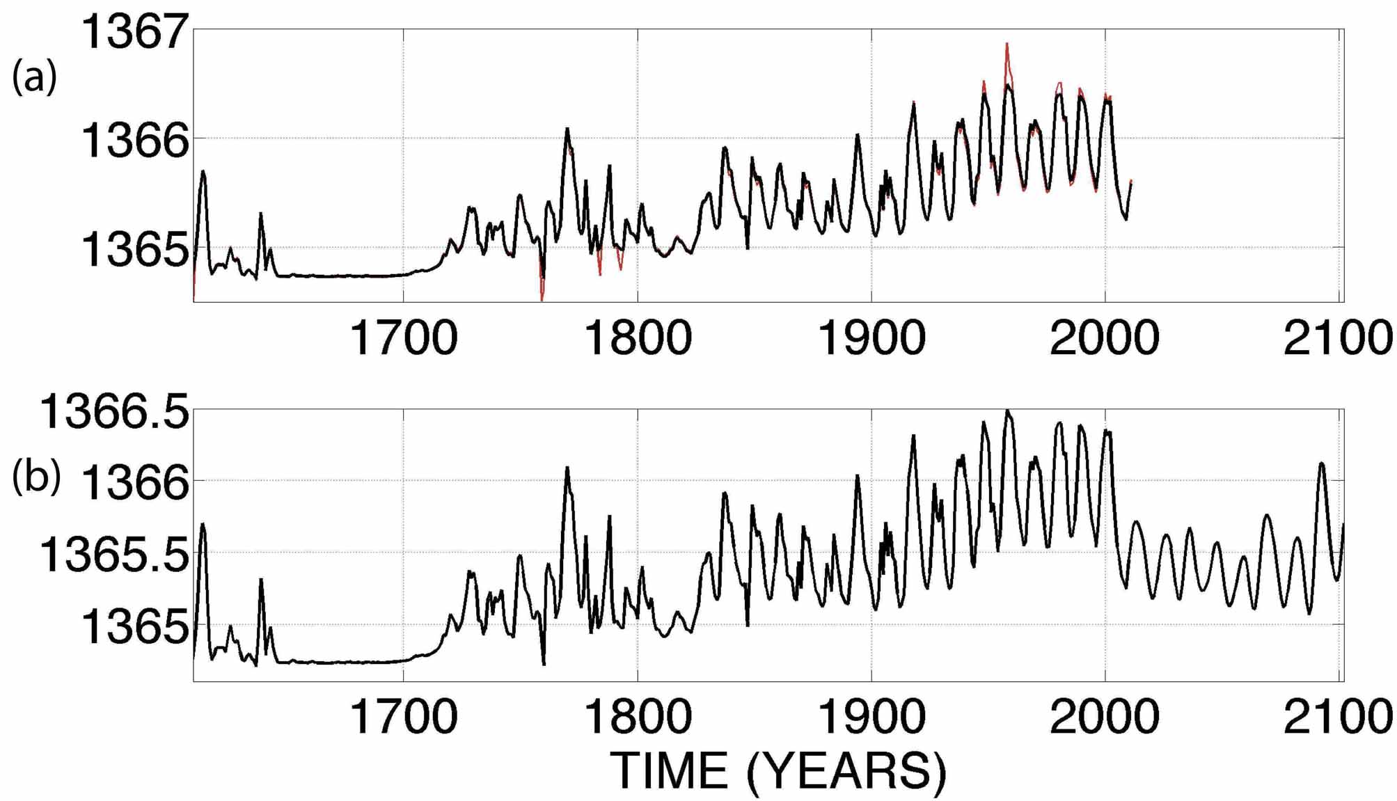
Figure 1: Time series. (a) The TSI-KRIVOVA-PMOD (red line) from $1610$ to $2010$ superposed on the times series estimated with the Least Squares Support Vector Machines (LS-SVM) between $1610$ and $2010$ (black line). (b) The LS-SVM model time series (black line) between $1610$ and $2100$

To project the TSI for the next hundred years, we use a method based on Least Squares Support Vector Machines (LS-SVM) with Nonlinear Autoregressive Exogenous (NARX) model and with radial basis function (RBF) kernel that allows a better precision in the estimation of the future values of a time series Vapnik (1998); Suykens et al. (2005).

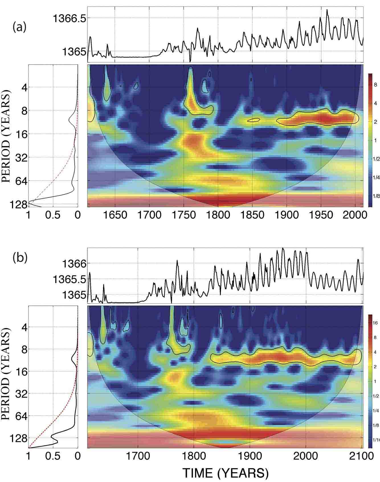
Figure 2: (a) Upper panel, TSI-KRIVOVA-PMOD; right panel spectral wavelet analysis; left panel global wavelet. (b) The same as in (a) but for the LS-SVM model.

Since the instrumental TSI records began in $1979$, we work with reconstructed TSI series. Long-term reconstructions of TSI Steinhilber et al. (2009); et al (2011) show epochs of maxima and minima when substantial changes in the TSI occur. These changes can contribute to climate variability et al (2010) and new estimate of the TSI for the 21st century, will have an important impact on climate modeling.

We tested three TSI recent reconstructions. Two of them use a model based on the evolution of the Sun s total and open magnetic flux: The Wang reconstruction Y-M.Wang et al. (2005) consider differential rotation, supergranular convection and meridional flow; this model is used to derive two TSI reconstructions, one with and one without a secularly varying background; from $1850$ onwards these reconstructions are the recommended solar forcings for the fifth Coupled Model Intercomparison Project $20$th century simulations Taylor et al. (2009).

The Krivova reconstruction Krivova et al. (2010) relies on time constants representing the decay and conversion of the different photospheric magnetic flux components. The Stenhilber reconstructionSteinhilber et al. (2009), uses the observationally derived relationship between TSI and the open solar magnetic field, the latter obtained from the cosmogenic radionuclide ${}^{10}Be$.

However, the best reconstruction to apply our method is the Krivova reconstruction Krivova et al. (2010) because it has a better temporal and spectral resolution compared to the Stenhilber reconstruction Steinhilber et al. (2009) and the correlation between the reconstructed and the PMOD composite is better than the Wang reconstructionY-M.Wang et al. (2005).

From $1610$ to $1975$ we use the Krivova reconstruction Krivova et al. (2010) and from $1976$ to $2010$ we use the PMOD composite. In this work we use the TSI-KRIVOVA-PMOD between 1610 and 2010.

To search for the future TSI values, the NARX LS-SVM was trained with $80\%$ of random data of the TSI-KRIVOVA-PMOD, obtaining a mean squared error (MSE) of $0.0084$, the testing of the remaining $20\%$ presents an MSE of $0.0073$.

We plot the TSI-KRIVOVA-PMOD with red line and the NARX LS-SVM model with black line in Fig. $1a$. It is clear that the NARX LS-SVM model (black line) reproduces very well the TSI-KRIVOVA-PMOD; the linear correlation coefficient between the TSI-KRIVOVA and the NARX LS-SVM model series for $1610$-$1975$ is $r=0.9969$, while $r$ value for the PMOD and the NARX LS-SVM model for $1976$-$2010$ interval is $0.9959$.

In Fig. $1b$ we present the NARX LS-SVM future TSI estimation (black line) between $2011$ and $2100$ with standard deviation $\sigma=0.4318$ $Wm^{-2}$. We notice a decreasing trend of the TSI between $2003$ and $2063$, coinciding with other types of prediction adopting different methodsV.M.Velasco et al. (2008); M. Lockwood and A.P. Rouillard and I.D. Finch (2009); et al. (2010, 2010).

However, it is not enough to conclude that the amplitudes among the reconstructed, the composite and the modeled time series are similar, it is also necessary to compare the spectral characteristics.

We apply the wavelet analysis using the Morlet function Torrence and Compo (1998), to quantify the TSI time series till 2100 A.D. and to analyse local variations of multiple periodicities. This method provides a higher resolution of periodicity, allows us to calculate the phase, and to filter the TSI in bandwidths et al. (2011).

Also, to calculate the confidence level we used the normalizepdf function, in this way the TSI will have a gaussian distributionGrinsted et al. (2004). Wavelet meaningful periodicities (confidence level greater than $95\%$) must be inside the cone of influence (COI), which is the region of the wavelet spectrum outside which the edge effects become important Torrence and Webster (1999). We also include the global spectra in the wavelet plots to show the power contribution of each periodicity inside the COI Velasco and Mendoza (2008).

We established our significance levels in the global wavelet spectra with a simple red noise model (increasing power with decreasing frequency Gilman et al. (1963)). We only took into account those periodicities above the red noise level.

In Fig. $2$ we show the wavelet analysis for the TSI-KRIVOVA-PMOD (Fig. $2a$) and the NARX LS-SVM model (Fig. $2b$). In the central panel of Fig. $2a$ the $11$-years cycle appears attenuated during the secular minima and is stronger since $\sim$$1875$, while the $\sim$$120$-years cycle keeps a more or less uniform power along all the time-span considered, both periodicities appear above the red noise level in the global spectra (right panel). Fig. $2b$ shows roughly the same spectral evolution of Fig. $2a$ but the two peaks above the red noise level are the $11$-years and the $240$-years. Also Fig. $2b$ indicates that the $11$-years cycle will be attenuated during the next $60$ years (to $2063$), which is a characteristic of a secular minima.

In Fig. $3$ we show a further analysis of the amplitudes (black areas) and phases (blue lines), that allow us to quantify the starting and ending of a cycle of the NARX LS-SVM model and were obtained using the inverse wavelet transform Torrence and Compo (1998). Fig. $3b$ shows the $11$-years cycle, as sunspots were so scarce during the “Prolonged Sunspot Minimum”, it has been suggested that the solar dynamo stopped Charbonneau (2010); Ossendrijver (2003). The figure clearly shows the 11-years amplitude attenuated during the Maunder, Dalton and Modern minima (negative phase of the periodicity of 120-years in Fig. 3c). The amplitude of the solar cycle never disappears completely, this is particularly so during the Maunder minimum Beer et al. (1998). After the year 2000 the peak amplitude of the cycle tends to decrease, in fact during the 21st minimum ($2003$$-$$2063$) it is similar to the Dalton or Modern minima ($1883$$-$$1940$).

The phase also shows an amplitude modulation, it presents an inversion between $\sim$$1780$ and $1790$, as this in not a particularly maximum or minimum time, we suggest that it comes probably from a shortcoming of the TS-KRIVOVA reconstruction in this time-interval.

From $2011$ to $2100$, the phase does not show any other inversion, probably indicating the good quality of our estimation. Fig. $3c$ shows the $120$-years cycle, we notice that it is the negative phase of this periodicity that coincides with the secular minima: Maunder between the years $1637$$-$$1704$, Dalton between the years $1771$$-$$1829$ , Modern between the years $1883$$-$$1940$ and the $21$st century minima between the years $2003$ and $2063$.

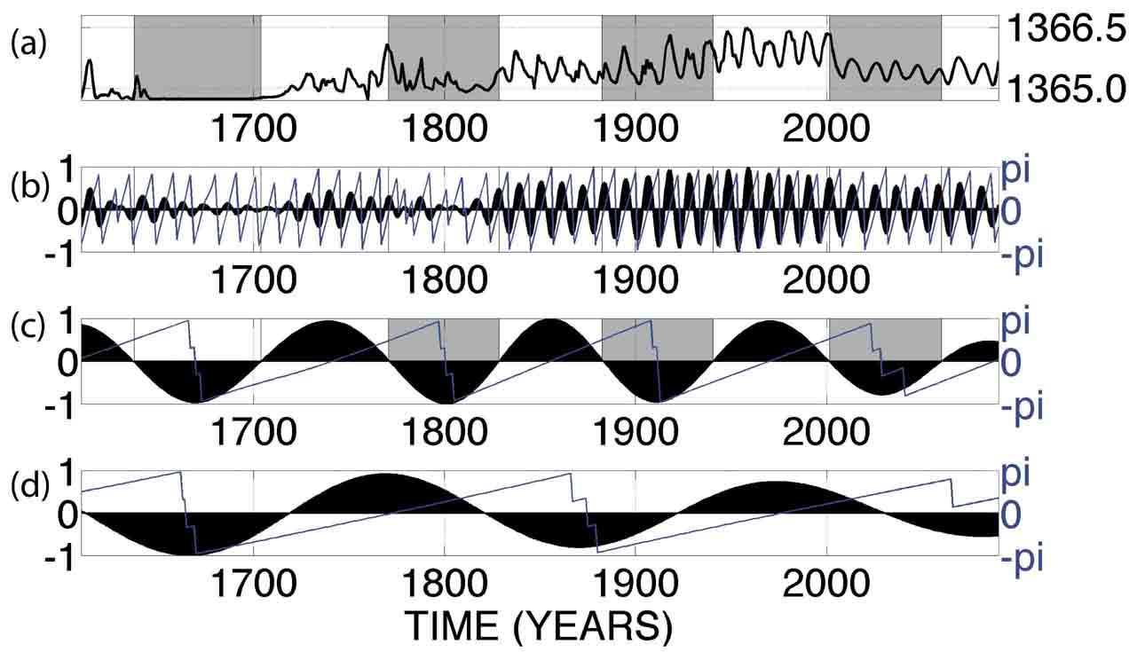
Figure 3: Phases (blue lines) and amplitudes (black areas) associated to the main periodicities of the LS-SVM model. The light-gray shading indicates the time-span of the secular minima. (a) Modeled time series . (b) The $11$-yrs cycle. (c) The $120$-yrs cycle. (d) The $240$-yrs cycle.

Based on this periodicity we calculate the average TSI for the secular minima: Maunder $1364.8$ $Wm^{-2}$, Dalton $1365.2$ $Wm^{-2}$ Modern $1365.5$ $Wm^{-2}$ and the $21$ st century $1365.4$ $Wm^{-2}$ $\pm$ $1\sigma=0.4318$ $Wm^{-2}$, this TSI value is between the Dalton and Modern minima. Again we observe that the phase does not change after $2010$.

The Modern maximum noticed between the years $1940$ and $2003$ has an average TSI of $1366$ $Wm^{-2}$, and the $21$st century minimum has a TSI average of $1365.4$ $Wm^{-2}$, this implies a negative radiative forcing of $\sim$$-0.1$ $Wm^{-2}$. The radiative forcing for the Maunder minimum to the Modern maximumKrivova et al. (2010) is $\sim$$0.21$ $Wm^{-2}$, then the radiative forcing associated to the $21$st century minimum is almost half of that forcing.

Finally, Fig. $3d$ shows the $240$-years cycle, it seem that according to the lag between the $120$-years and $240$-years cycles we have different amplitudes of the secular solar minima, for instance, when its negative phase coincides with the $120$-years cycle we have the deepest minima, like the Maunder minimum. Again, the phase of this periodicity holds for the next $100$ years.

To decide when the solar activity is “high” or “low”, we calculate the power of the TSI as a direct indicator of energy released by the solar dynamo and the level of activity for each solar cycle. We use the mean power value of the PMOD composite ($1976-2010$) to calculate the anomalies for each cycle. The power anomalies are normalized and appear as blue bars in Fig. 4, which also presents the TSI (solid line). There are positive power anomalies during solar cycles $21$ and $22$, coinciding with the end of the Modern maximum. Between solar cycles $23$ and $30$ the power anomalies are negative, coinciding with negative phase of the $120$-years periodicity. This reinforces the result of Fig. 3c suggesting that this periodicity is closely associated with secular minima. According to the power of the anomalies, solar cycles $23$–$25$ and $30$ could present lower activity than cycles $26$ to $29$, regardless of the fact that the peaks of cycles 27 and 28 are the lowest.

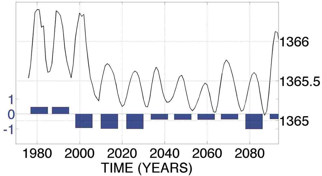
Figure 4: We use the mean power PMOD composite (1976-2010) to calculate the power anomaly for each cycle. The power anomalies are normalized and appear as blue bars. The TSI is the solid line. Negative (or Positive) power anomalies is ‘Low” (or “High”) solar activity

The calculated power anomalies show that low solar secular activity occurs when there are negative anomalies and high solar secular activity appears with positive anomalies. It is possible that the zero in the anomalies, represents the normal state of the dynamo. The “Prolonged Sunspot Minimum” discovered by Maunder, represents a phase of solar history and corresponds to a special state of the dynamo when it is working well below its average power.

This work was partially supported by DGAPA-UNAM, IN$103209-3$, IN$117009-3$, IN$105909$ and IN$117009$ grants, IXTLI: IX$101010$ and IX$100810$ grants and CONACYT-F$282795$ grant.

References

- Schwabe (1843) V. H. H. Schwabe, Astronomische Nachrichten, 473, 283–284 (1843).
- Maunder (1894) E.W. Maunder, Mon. Not. R. Astrom. Soc, 17, 173–176 (1894).
- Eddy (1976) J.A. Eddy, Science, 192 (4245), 1189–1202 (1976).
- Petrovary (2010) K. Petrovary, Living Rev. Solar Phys., 7 (2010).
- Charbonneau (2010) P. Charbonneau, Living Rev. Solar Phys., 7 (2010).
- Ossendrijver (2003) M. Ossendrijver, Astron. Astrophys. Rev., 11, 287–367 (2003).
- Mendoza and V.M.Velasco (2011) B. Mendoza and V.M.Velasco, Solar Physics, 271, 169–182 (2011).
- V.M.Velasco et al. (2008) V.M.Velasco, B. Mendoza, and J.F. Valdés-Galicia, Proceedings of the 30th International Cosmic Ray Conference, 1 (SH), 553–556 (2008).
- Tobias et al. (2004) S.M. Tobias, N.O. Weiss, and J. Beer., Astron. Geophys., 45, 2.6 (2004).
- Hale (1908) G. E. Hale, The Astrophysical Journal., 28, 315–343 (1908).
- M.S. Kirk, M.S. and W.D. Pesnell and C.A. Young and S.A. Hess-Webber (2009) M.S. Kirk, M.S. and W.D. Pesnell and C.A. Young and S.A. Hess-Webber, Solar Physics, 257, 99–112 (2009).
- C.O. Lee (2009) C.O. Lee, Solar Physics, 256, 345–363 (2009).
- E.J. Smith and A. Balogh (2008) E.J. Smith and A. Balogh, Geophys. Res. Lett., 35, L22103 (2008).
- D.J. McComas et al. (2008) D.J. McComas et al., Geophys. Res. Lett., 35, L18103 (2008).
- C. Fröhlich (2009) C. Fröhlich, Astron. Astrophys., 501, L27–L30 (2009).
- Fröhlich (2006) C. Fröhlich, Space Sci. Rev., 125, 53–65 (2006).
- Foukal et al. (2009) P. C. Foukal, H. Fr hlich, Spruit, and T.M.M. Wigley, Geophys. Res. Lett., 36, L19704 (2009).
- Usoskin et al. (2003) I.G. Usoskin, S.K. Solanki, M. Schussler, K. Mursula, and K. Alanko, Phys. Rev. Lett., 91, 211101, 211101 (2003).
- M. Lockwood and A.P. Rouillard and I.D. Finch (2009) M. Lockwood and A.P. Rouillard and I.D. Finch, Astrophys. J., 700, 937–944 (2009).
- et al. (2010) J.A. Abreu et al., Geophys. Res. Lett., 48, RG2004 (2010a).
- Russell et al. (1986) C.T. Russell, J.G. Luhmann, and L.K. Jian., Rev. Geophys., 320, 735–738 (1986).
- et al. (2010) N.R.Rigozo et al., Planetary and Space Sci., 58, 1971–1976 (2010b).
- Pesnell (2008) W.D. Pesnell, Living Rev. Solar Phys., 7(6) (2008).
- Vapnik (1998) V. Vapnik, Statistical Learning Theory (Jhon Wiley & Sons, New York., 1998).
- Suykens et al. (2005) J.A.K. Suykens, T.V. Gestel, J. De Brabanter, B. De Moor, and J. Vandewalle, Least-Squares Support Vector Machines (World Scientific Publishing Co. Pte. Ltd, 2005).
- Steinhilber et al. (2009) A.I. Steinhilber, J. Beer, and C. Fröhlich, Geophys. Res. Lett., 36, L19704 (2009).
- et al (2011) A.I. Shapiro et al, Astron. Astrophys., 529, A67 (2011).
- et al (2010) L.J. Gray, et al, Rev. Geophys, 48, RG4001 (2010).
- Y-M.Wang et al. (2005) Y-M.Wang, J. L. Lean, and N.R. Sheeley Jr., Astrophys. J., 625, 522–538 (2005).
- Taylor et al. (2009) K.E. Taylor, R.J. Stouffer, and G.A. Meehl, http:cmip-pcmdi.llnl.gov/cmip5/docs/TaylorCMIP5design.pdf (2009).
- Krivova et al. (2010) N.A. Krivova, L.E.A. Vieira, and S.K. Solanki., Journal of Geophysical Research, 115, A12112, 11 (2010).
- Torrence and Compo (1998) C. Torrence and G.P. Compo, Bull. Am. Meteorol. Soc., 79, 61–78 (1998).
- et al. (2011) W Soon et al., Journal of Atmospheric and Solar-Terrestrial Physics, 73, 2331–2344 (2011).
- Grinsted et al. (2004) A. Grinsted, J. Moore, and S. Jevrejera, Nonlinear Process. Geophys., 11, 561 566 (2004).
- Torrence and Webster (1999) C. Torrence and P. Webster, J. Clim., 12, 2679–2690. (1999).
- Velasco and Mendoza (2008) V.M. Velasco and B. Mendoza, Advances in Space Research, 12, 866–878 (2008).
- Gilman et al. (1963) D.L. Gilman, F.H. Fuglister, and J.M. Mitchell, J. Atmos. Sci., 20, 182–184 (1963).
- Beer et al. (1998) J. Beer, S.M. Tobias, and N.O. Weiss, Solar Physics, 181, 237–249 (1998).