Cylinder with Charged Anisotropic Source

Abstract

We take charged anisotropic fluid cylinder when there is no external pressure acting on the fluid. This is a cylindrical version of the Krori and Barua’s method to explore the field equations with anisotropic fluid. We discuss models with positive matter density and pressure that satisfy all the energy and stability conditions. It is found that charge does not vanish at the center of the cylinder. The equilibrium condition as well as physical conditions are discussed. Further, we highlight the connection between our solutions and the charged strange quark stars as well as with dark matter including charged massive particles. The graphical analysis of the matter variables versus charge is given which indicates a physically reasonable matter distribution.

Keywords: Field equations; Equation of state; Charged anisotropic source.
PACS: 04.40.Nr; 04.40.Dg; 04.20.Jb

1 Introduction

The study of general relativistic charged compact objects is of fundamental importance in astrophysics. Strong magnetic fields, different kinds of phase transitions and solid stellar core cause anisotropy in the fluids. However, charged fluids with anisotropy complicates the solution of the field equations. Equations of state (EoS) has important consequences in such situations. Many exact solutions have been obtained [1] by using a simple form of the energy-momentum tensor and assuming some symmetries.

There have been pervious discussions of a similar nature by Evan [2], Bronnikov [3], Latelier and Tobensky [4], and Kramer [5]. They used various EoS that could be written in the form $\rho=\gamma p$ for specific positive values of $\gamma$, as well as energy conservation. Some work has been done on charged anisotropic static matter by using spherically symmetric stars with the linear, nonlinear and Chaplygin gas EoS. Ivanov [6] showed that the field equations can be simplified by using linear EoS for a charged perfect fluid but with non-integrable equations. Sharma and Maharaj [7] explored the field equations for static spherically symmetric uncharged anisotropic fluid with combined linear EoS and a particular mass function.

Charged anisotropic fluids have been discussed in General Relativity since the pioneering work of Bonner [8]. Ray et al. [9] investigated charged anisotropic spheres with Chaplygin gas EoS. Thirukkanesh and Maharaj [10] generated models for charged anisotropic spherically symmetric stars by using linear EoS as well as choosing one of the metric functions and electric field intensity. Horvat et al. [11] studied gravastars for charged anisotropic fluid. Recently, Victor et al. [12] explored solutions for the charged anisotropic spheres with linear or nonlinear EoS.

Over the years, many authors have proposed various formulations to solve the field equations for cylindrically symmetric spacetime. Nilsson et al. [13] investigated cylindrically symmetric perfect fluid models. One of the authors (MS) [14] explored perfect fluid, static cylindrically symmetric solutions of the field equations by using different EoS. Sharif and Fatima [15] worked for the charged anisotropic cylinder but they discussed gravitational collapse. Som [16] explored the charged dust cylinder. However, there has been a little progress towards investigating charged anisotropic static cylindrically symmetric solutions with or without using an EoS.

In a recent paper [17], we have explored exact solutions of the field equations for the charged anisotropic static cylindrically symmetric spacetime using Thirukkanesh and Maharaj [10] approach. Here we extend this study for the charged anisotropic static cylindrically symmetric spacetime by using Victor et al. [12] procedure. A system of differential equations for matter as well as electric field intensity and anisotropic pressures are solved on the basis of linear and nonlinear EoS. Numerical factors depending on matching conditions are used with each EoS which provide relationship among charge distribution, pressure anisotropy and EoS.

The outline of the paper is as follows: In the next section, we write down the Einstein-Maxwell field equations for the static cylindrically symmetric spacetime and also express this system of equations with original Krori and Barua’s [18] assumptions. We apply the central and boundary conditions on electric field intensity and radial pressure respectively to analyze these field equations at center and on the boundary of the cylinder. Section 3 investigates models for linear, nonlinear and Chaplygin gas EoS by taking positive matter densities and pressures corresponding to the relevant EoS. In section 4, we match smoothly the interior and exterior metrics and bring adimesionality in the three models. Section 5 provides some physical features of these models. In particular, we discuss the stability conditions, energy conditions, the ven der Waals EoS [19] and the equilibrium conditions for our models. The last section 6 contains concluding remarks about the results.

2 The Field Equations

We take the static cylindrically symmetric spacetime given by [20]

$$ds^{2}=e^{2\nu}dt^{2}-e^{2\mu-2\nu}dr^{2}-r^{2}e^{-2\nu}d\phi^{2}-e^{2\mu-2\nu}dz^{2},$$ (1)

where $\nu$ and $\mu$ are functions of $r$. The transformation $d\phi=e^{\nu}d\theta$ leads the above equation to the following form [13, 15]

$$ds^{2}=e^{2\nu}dt^{2}-e^{2\mu-2\nu}dr^{2}-r^{2}d\theta^{2}-e^{2\mu-2\nu}dz^{2}.$$ (2)

The field equations for the charged anisotropic source are

$$R_{ab}-\frac{1}{2}g_{ab}R=\kappa(T^{(m)}_{ab}+T^{(em)}_{ab}),$$ (3)

where $T^{(m)}_{ab}$ and $T^{(em)}_{ab}$ are the energy-momentum tensors for anisotropic matter and electromagnetic field respectively. The energy-momentum tensor for anisotropic fluid is

$$T^{(m)}_{ab}=(\rho+p_{r})u_{a}u_{b}-p_{t}g_{ab}+(p_{t}-p_{r})\eta_{a}\eta_{b}$$ (4)

satisfying $u^{a}u_{a}=-\eta^{a}\eta_{a}=1$, where $\rho$ is the charge density, $p_{r}$ is the radial pressure, $p_{t}$ is the tangential pressure, $u_{a}=e^{\nu}\delta^{0}_{a}$ is the 4-velocity and $\eta_{a}=-e^{\mu-\nu}\delta_{a}^{1}$ is the 4-unit vector. The energy-momentum tensor for the electromagnetic field is

$$T^{(em)}_{ab}=\frac{1}{4\pi}(-g^{cd}F_{ac}F_{bd}+\frac{1}{4}g_{ab}F_{cd}F^{cd}),$$ (5)

where $F_{ab}=A_{b,a}-A_{a,b}$ is the Maxwell field tensor and $A_{a}$ is the 4-potential. The Maxwell field equations are given by

$$[\sqrt{-g}F^{ab}]_{,b}=4\pi J^{a}\sqrt{-g},\quad F_{[ab,c]}=0,$$ (6)

where $J^{a}=\sigma u^{a}$ is the 4-current of the fluid element and $\sigma$ is the proper charge density.

The field equations for the line element (2) become

$$e^{2\nu-2\mu}(\nu^{\prime\prime}-\mu^{\prime\prime})=8\pi\rho+E^{2},$$ (7)

$$\frac{e^{2\nu-2\mu}}{r}(-r\nu^{\prime 2}+r\nu^{\prime}\mu^{\prime}+\mu^{\prime})=8\pi p_{r}-E^{2},$$ (8)

$$e^{2\nu-2\mu}(\nu^{\prime}~{}^{2}+\mu^{\prime\prime})=8\pi p_{t}+E^{2},$$ (9)

$$\sigma=\frac{e^{2\nu-2\mu}}{4\pi r}(re^{\mu-\nu}E)^{\prime},$$ (10)

where prime denotes differentiation with respect to $r$ and $E=2\sqrt{\pi}e^{-\mu}\frac{\partial A}{\partial r}$ stands for em part. In the system of equations (7)-(10), there are seven unknowns, so we make physically reasonable choices for any two of the unknowns. We take the gravitational potential $e^{2\mu-2\nu}$ and the electric field intensity $E$ as [11]

$$e^{2\mu-2\nu} = \frac{1+(c_{1}-c_{2})r}{1+c_{1}r},$$ (11)

$$E^{2} = \frac{k(3+c_{1}r)}{(1+c_{1}r)^{2}},$$ (12)

where $c_{1},~{}c_{2}$ and $k$ are constants. Substituting Eqs.(11) and (12) in Eq.(10), we obtain

$$\sigma\approx\frac{\sqrt{3k}}{2\pi r}.$$ (13)

This shows that there is a singularity in the charge distribution at $r=0$. However, this choice keeps the charge distribution regular at the centre of the cylinder as $E(r)$ remains finite there (12).

The singularity free models for charged anisotropic static cylinder are constructed by taking [18]

$$\mu=Ar^{2},\quad\nu=Br^{2}+C,$$ (14)

where $A,~{}B$ and $C$ are constants. Using these values in Eqs.(7)-(10), it follows that

$$e^{2r^{2}(B-A)+2C}(2B-2A)=8\pi\rho+E^{2},$$ (15)

$$e^{2r^{2}(B-A)+2C}(-4B^{2}r^{2}+4ABr^{2}+2A)=8\pi p_{r}-E^{2},$$ (16)

$$e^{2r^{2}(B-A)+2C}(4B^{2}r^{2}+2A)=8\pi p_{t}+E^{2},$$ (17)

$$\sigma=\frac{e^{2r^{2}(B-A)+2C}}{4\pi r}(re^{r^{2}(A-B)-C}E)^{\prime}.$$ (18)

Now we impose the central and boundary conditions on $E(r)$ and $p_{r}(r)$ respectively as follows:

$$E(0)=0,\quad p_{r}(a)=0,$$ (19)

where $a$ is a positive constant and $r=a$ is the interface of the charged fluid and vacuum (i.e., boundary of the cylinder). We apply central conditions to the system of Eqs.(15)-(17), it follows that

$$\rho(0)=\frac{(B-A)e^{2C}}{4\pi},\quad p_{r}(0)=\frac{Ae^{2C}}{4\pi},\quad p_{t}(0)=\frac{Ae^{2C}}{4\pi}.$$ (20)

This shows that $p_{r}(r)=p_{t}(r)$ at $r=0$, hence the anisotropy of the cylinder vanishes at the center. Applying the boundary conditions to Eqs.(15)-(17), we get

$$\rho(a) = \frac{e^{2a^{2}(B-A)+2C}(-2B^{2}a^{2}+B+2ABa^{2})}{4\pi},$$ (21)

$$p_{t}(a) = \frac{e^{2a^{2}(B-A)+2C}(A+ABa^{2})}{2\pi},$$ (22)

$$E^{2}(a) = e^{2a^{2}(B-A)+2C}(4ABa^{2}+2A-4B^{2}a^{2}).$$ (23)

The general expressions for $p_{t}$ and $E^{2}$ from Eqs.(15)-(17) are

$$p_{t}(r) = \frac{e^{2r^{2}(B-A)+2C}(-2B+2B^{2}r^{2}+2A)}{4\pi}+\rho,$$ (24)

$$E^{2}(r) = e^{2r^{2}(B-A)+2C}(2B-2A)-8\pi\rho.$$ (25)

3 Models for Equations of State

The general form of EoS is

$$p_{r}=p_{r}(\rho,a_{1},a_{2}),$$ (26)

where $a_{1}$ and $a_{2}$ are parameters constrained by

$$p_{r}(0)=p_{r}[\rho(0),a_{1},a_{2}],\quad 0=p_{r}[\rho(a),a_{1},a_{2}].$$ (27)

Adding Eqs.(15) and (16), we obtain

$$\rho+p_{r}=\frac{e^{2r^{2}(B-A)+2C}}{8\pi}(-4B^{2}r^{2}+2B+4ABr^{2})\equiv l(r).$$ (28)

This equation may be used with the assumed EoS to find $\rho$ and $p_{r}$. The corresponding value of $\rho$ will be used in Eqs.(24) and (25) to evaluate $p_{t}$ and $E^{2}$ respectively. In the following we discuss three types of EoS:

3.1 The Linear EoS

This is given by

$$p_{r}=\alpha_{1}+\alpha_{2}\rho,$$ (29)

where $\alpha_{1},~{}\alpha_{2}$ are constants. Using this EoS, we obtain expressions for $\rho,~{}p_{r},~{}p_{t}$ and $E^{2}$ as follows:

$$\rho = \frac{e^{2r^{2}(B-A)+2C}(-4B^{2}r^{2}+2B+4ABr^{2})-8\pi\alpha_{1}}{8\pi(1+\alpha_{2})},$$ (30)

$$p_{r} = \frac{\alpha_{2}e^{2r^{2}(B-A)+2C}(-4B^{2}r^{2}+2B+4ABr^{2})+8\pi\alpha_{1}}{1+\alpha_{2}}.$$ (31)

Using Eq.(30) in Eqs.(24) and (25) successively, we get

$$p_{t} = \frac{e^{2r^{2}(B-A)+2C}((2B-4A-4B^{2}r^{2})(1+\alpha_{2})+4B^{2}r^{2}-4ABr^{2}-2B)}{8\pi(1+\alpha_{2})}$$ (32)

$$- \frac{\alpha_{1}}{1+\alpha_{2}},$$

$$E^{2} = \frac{e^{2r^{2}(B-A)+2C}((2B-2A)(1+\alpha_{2})+4B^{2}r^{2}-4ABr^{2}-2B)}{1+\alpha_{2}}-\frac{8\pi\alpha_{1}}{1+\alpha_{2}}.$$

The values of constants $\alpha_{1}$ and $\alpha_{2}$ are found by solving Eqs.(27) and (29) as

$$\alpha_{1}=-\frac{\rho(a)p_{r}(0)}{\rho(0)-\rho(a)},\quad\alpha_{2}=\frac{p_{r}(0)}{\rho(0)-\rho(a)}.$$ (34)

3.2 The Nonlinear EoS

The nonlinear EoS is given by

$$p_{r}=\beta_{1}+\frac{\beta_{2}}{\rho^{n}},$$ (35)

where $n\neq-1$ and $\beta_{1},~{}\beta_{2}$ are constants. It is a modification of the Chaplygin gas EoS used by Bertolami and Paramos [21] to describe neutral dark stars. For $n=1$, Eqs.(28) and (35) lead to

$$\rho=\frac{l(r)-\beta_{1}\pm\sqrt{(l(r)-\beta_{1})^{2}-4\beta_{2}}}{2}.$$ (36)

Substituting Eq.(36) in Eqs.(35), (24) and (25) respectively, it follows that

$$p_{r} = \beta_{1}+\frac{2\beta_{2}}{l(r)-\beta_{1}\pm\sqrt{(l(r)-\beta_{1})^{2}-4\beta_{2}}},$$ (37)

$$p_{t} = \frac{e^{2r^{2}(B-A)+2C}(-B+2B^{2}r^{2}+2A)}{4\pi}$$ (38)

$$+ \frac{l(r)-\beta_{1}\pm\sqrt{(l(r)-\beta_{1})^{2}-4\beta_{2}}}{2},$$

$$E^{2}(r) = e^{2r^{2}(B-A)+2C}(2B-2A)-4\pi\left(l(r)-\beta_{1}\right.$$ (39)

$$\pm \left.\sqrt{(l(r)-\beta_{1})^{2}-4\beta_{2}}\right),$$

where $l(r)$ is given by Eq.(28). The constants $\beta_{1}$ and $\beta_{2}$ are found from Eqs.(35) and (27) as

$$\beta_{1}=\frac{\rho(0)p_{r}(0)}{\rho(0)-\rho(a)},\quad\beta_{2}=-\frac{\rho(0)\rho(a)p_{r}(0)}{\rho(0)-\rho(a)}.$$ (40)

Equation (36) implies that $\beta_{2}$ must be negative so that each root in this equation has definite sign which will correspond to a positive definite matter density.

3.3 The Modified Chayplygin Gas EoS

This EOS has the following form

$$p_{r}=\gamma_{1}\rho+\frac{\gamma_{2}}{\rho},$$ (41)

where $\gamma_{1},~{}\gamma_{2}$ are constants. This is used to describe static, neutral, phantom-like sources [22]. Using this EoS with Eq.(28), we get

$$\rho=\frac{l(r)\pm\sqrt{l(r)^{2}-4(1+\gamma_{1})\gamma_{2}}}{2(1+\gamma_{1})}.$$ (42)

Substituting this value of $\rho$ in Eq.(41) as well as in Eqs.(24) and (25) successively, it follows that

$$p_{r} = \gamma_{1}\left(\frac{l(r)\pm\sqrt{l(r)^{2}-4(1+\gamma_{1})\gamma_{2}}}{2(1+\gamma_{1})}\right)$$ (43)

$$+ \frac{2\gamma_{2}(1+\gamma_{1})}{l(r)\pm\sqrt{l(r)^{2}-4(1+\gamma_{1})\gamma_{2}}},$$

$$p_{t} = \frac{e^{2r^{2}(B-A)+2C}(-B+2B^{2}r^{2}+2A)}{4\pi}$$ (44)

$$+ \frac{l(r)\pm\sqrt{l(r)^{2}-4(1+\gamma_{1})\gamma_{2}}}{2(1+\gamma_{1})},$$

$$E^{2} = e^{2r^{2}(B-A)+2C}(2B-2A)$$ (45)

$$- 4\pi\left(\frac{l(r)\pm\sqrt{l(r)^{2}-4(1+\gamma_{1})\gamma_{2}}}{1+\gamma_{1}}\right),$$

where $\gamma_{1}$ and $\gamma_{2}$ are

$$\gamma_{1}=\frac{\rho(0)p_{r}(0)}{\rho(0)^{2}-\rho(a)^{2}},\quad\gamma_{2}=-\frac{\rho(0)p_{r}(0)\rho(a)^{2}}{\rho(0)^{2}-\rho(a)^{2}}.$$ (46)

For $(1+\gamma_{1})<0$ and $\gamma_{2}>0$ or $(1+\gamma_{1})>0$ and $\gamma_{2}<0$, Eq.(42) yields roots of definite sign which will again correspond to the positive matter densities. It is clear that the positive or negative matter densities depend upon the positivity or negativity of the constants $\beta_{1},~{}\beta_{2},~{}\gamma_{1}$ and $\gamma_{2}$, i.e., the roots of Eqs.(36) and (42) respectively.

4 Matching Conditions and Adimensional Matter Sources

Here we take the charged static cylindrically symmetric spacetime as an exterior region given by [23]

$$ds^{2}=N(r)dt^{2}-\frac{1}{N(r)}dr^{2}-r^{2}d\theta^{2}-r^{2}d\psi^{2},\quad N(r)=\frac{q^{2}}{r^{2}}-\frac{2m}{r},$$ (47)

where $q$ and $m$ are charge and mass respectively. Using the transformation, $d\psi=\frac{1}{\sqrt{N(r)}}d\phi$, this takes the form

$$ds^{2}=N(r)dt^{2}-\frac{1}{N(r)}dr^{2}-r^{2}d\theta^{2}-\frac{r^{2}}{N(r)}d\phi^{2}.$$ (48)

With the radial transformation $r=\frac{m^{2}-q^{2}}{r^{\prime}}$, it becomes

$$ds^{2}=\frac{\frac{q^{2}}{r^{\prime 2}}-\frac{2m^{3}}{r^{\prime 3}}+\frac{2mq^{2}}{r^{\prime 3}}}{(\frac{m^{2}-q^{2}}{r^{\prime 2}})^{2}}dt^{2}-\frac{(\frac{m^{2}-q^{2}}{r^{\prime 2}})^{4}}{\frac{q^{2}}{r^{\prime 2}}-\frac{2m^{3}}{r^{\prime 3}}+\frac{2mq^{2}}{r^{\prime 3}}}(dr^{\prime 2}+d\phi^{2})-r^{\prime 2}d\theta^{2}.$$ (49)

To match the interior metric (2) with the exterior (49), we impose the continuity of $g_{00},~{}g_{11}$ and $\frac{\partial g_{00}}{\partial r}$ across a surface at $r^{\prime}=a$ by using the procedure [24]. In our case, this yields the following expressions for $A,~{}B$ and $C$ in terms of adimensional parameters $\eta=\frac{m}{a}$ and $\chi=\frac{|q|}{a}$ as

$$A = \frac{\ln(\eta^{2}-\chi^{2})}{a^{2}(\eta^{2}-\chi^{2})^{2}},$$ (50)

$$B = -\frac{1}{a^{2}(\eta^{2}-\chi^{2})}(\frac{1}{2}+\frac{\chi^{2}}{4(\chi^{2}-2\eta^{3}+\eta\chi^{2})}),$$ (51)

$$C = \frac{1}{2}+\frac{\chi^{2}}{4(\chi^{2}-2\eta^{3}+\eta\chi^{2})}+\ln\frac{\eta^{2}-\chi^{2}}{\sqrt{\chi^{2}-2\eta^{3}+\eta\chi^{2}}}.$$ (52)

We can see from Eq.(14) that $A$ and $B$ have dimension of $length^{-2}$ and $C$ is dimensionless. It is very important that the field equations can eventually be expressed in terms of these adimensional constants and the dimensionless radial coordinate $x=\frac{r}{a}$. Here adimesionality is denoted by $hats$. We assume that the interior of the fluid cylinder is described by $x\in[0,1)$. We reformulate all models as adimensional models where we are denoting $\hat{A}=a^{2}A,~{}\hat{B}=a^{2}B,~{}\hat{\rho}=a^{2}\rho,~{}\hat{p}_{r}=a^{2}p_{r},~{}\hat{p}_{t}=a^{2}p_{t},~{}\hat{E}^{2}=a^{2}E^{2}$ and $\hat{\sigma}=a^{2}\sigma$. The quantities which are originally dimensionless are denoted by the actual symbol. The central and the boundary conditions at $x\in[0,1)$ become

$$\hat{\rho}(0) = \frac{(\hat{B}-\hat{A})e^{2C}}{4\pi},$$ (53)

$$\hat{p_{r}}(0) = \frac{\hat{A}e^{2C}}{4\pi},$$ (54)

$$\hat{p_{t}}(0) = \frac{\hat{A}e^{2C}}{4\pi},$$ (55)

$$\hat{\rho}(1) = \frac{e^{2(\hat{B}-\hat{A})+2C}(2\hat{B}^{2}-\hat{B}-2\hat{A}\hat{B})}{4\pi},$$ (56)

$$\hat{p}_{t}(1) = \frac{e^{2(\hat{B}-\hat{A})+2C}(\hat{A}+\hat{A}\hat{B})}{2\pi},$$ (57)

$$\hat{E}^{2}(1) = e^{2(\hat{B}-\hat{A})+2C}(4\hat{A}\hat{B}+2\hat{A}-4\hat{B}^{2}).$$ (58)

The Adimensional linear EoS model

The adimensional linear EoS is given by

$$\hat{p}_{r} = \hat{\alpha}_{1}+\alpha_{2}\hat{\rho}.$$ (59)

The corresponding quantities will become

$$\hat{\rho} = \frac{e^{2x^{2}(\hat{B}-\hat{A})+2C}(-4\hat{B}^{2}x^{2}+2\hat{B}+4\hat{A}\hat{B}x^{2})-8\pi\hat{\alpha}_{1}}{8\pi(1+\alpha_{2})},$$ (60)

$$\hat{p}_{r} = \frac{8\pi\hat{\alpha}_{1}+\alpha_{2}e^{2x^{2}(\hat{B}-\hat{A})+2C}(-4\hat{B}^{2}x^{2}+2\hat{B}+4\hat{A}\hat{B}x^{2})}{1+\alpha_{2}},$$ (61)

$$\hat{p}_{t} = \frac{e^{2x^{2}(\hat{B}-\hat{A})+2C}}{8\pi}(-2\hat{B}+4\hat{B}^{2}x^{2}+4\hat{A})+\hat{\rho},$$ (62)

$$\hat{E}^{2} = e^{2x^{2}(\hat{B}-\hat{A})+2C}(2\hat{B}-2\hat{A})-8\pi\hat{\rho},$$ (63)

where

$$\hat{\alpha}_{1}=-\frac{\hat{\rho}(1)\hat{p}(0)}{\hat{\rho}(0)-\hat{\rho}(1)},\quad\alpha_{2}=\frac{\hat{p}_{r}(0)}{\hat{\rho}(0)-\hat{\rho}(1)}.$$ (64)

The Adimensional Nonlinear EoS Model

Here we have

$$\hat{p}_{r} = \hat{\beta}_{1}+\frac{\hat{\beta}_{2}}{\hat{\rho}}.$$ (65)

For this model, the corresponding quantities take the form

$$\hat{\rho} = \frac{\hat{l}(x)-\hat{\beta}_{1}\pm\sqrt{(\hat{l}(x)-\hat{\beta}_{1})^{2}-4\hat{\beta}_{2}}}{2},$$ (66)

$$\hat{p}_{t} = \frac{e^{2x^{2}(\hat{B}-\hat{A})+2C}(-\hat{B}+2\hat{B}^{2}x^{2}+2\hat{A})}{4\pi}+\hat{\rho},$$ (67)

$$\hat{E}^{2} = e^{2x^{2}(\hat{B}-\hat{A})+2C}(2\hat{B}-2\hat{A})-8\pi\hat{\rho},$$ (68)

where $\hat{\beta}_{1}$ and $\hat{\beta}_{2}$ are

$$\hat{\beta}_{1}=\frac{\hat{\rho}(0)\hat{p}_{r}(0)}{\hat{\rho}(0)-\hat{\rho}(1)},\quad\hat{\beta}_{2}=-\frac{\hat{\rho}(0)\hat{\rho}(1)\hat{p}_{r}(0)}{\hat{\rho}(0)-\hat{\rho}(1)}.$$ (69)

The Adimensional Modified Chaplygin EoS Model

The adimensional modified Chaplygin EoS model

$$\hat{p}_{r} = \gamma_{1}\hat{\rho}+\frac{\hat{\gamma}_{2}}{\hat{\rho}}$$ (70)

yield the following quantities

$$\hat{\rho} = \frac{\hat{l}(x)\pm\sqrt{\hat{l}(x)^{2}-4(1+\gamma_{1})\hat{\gamma}_{2}}}{2(1+\gamma_{1})},$$ (71)

$$\hat{p}_{t} = \frac{e^{2x^{2}(\hat{B}-\hat{A})+2C}(-\hat{B}+2\hat{B}^{2}x^{2}+2\hat{A})}{4\pi}+\hat{\rho},$$ (72)

$$\hat{E}^{2} = e^{2x^{2}(\hat{B}-\hat{A})+2C}(2\hat{B}-2\hat{A})-8\pi\hat{\rho},$$ (73)

where

$$\gamma_{1}=\frac{\hat{\rho}(0)\hat{p}_{r}(0)}{\hat{\rho}^{2}(0)-\hat{\rho}^{2}(1)},\quad\hat{\gamma}_{2}=-\frac{\hat{\rho}(0)\hat{p}_{r}(0)\hat{\rho}^{2}(1)}{\hat{\rho}^{2}(0)-\hat{\rho}^{2}(1)}.$$ (74)

The adimensional proper charge density for all the above three models will become

$$\hat{\sigma}=\frac{e^{2x^{2}(\hat{B}-\hat{A})+2C}}{2\pi x}\frac{d}{dx}(xe^{x^{2}(\hat{B}-\hat{A})+2C}\hat{E}).$$ (75)

5 Some Features of the Models

In this section, we discuss some insights of the three models. The exterior metric (47) implies that singularity occurs at $r=0,~{}\frac{q^{2}}{2m}$. It is regular everywhere except at $r=0$ [23]. The surface with $r=\frac{q^{2}}{2m}$ describes a right singular circular cylinder. Using Eqs.(50)-(52) in $\rho(0)$ of Eq.(20), it turns out to be positive. Following [12], we have $\eta=\frac{GM}{c^{2}a}\approx 1.147$ for $M$ to be the solar mass and $a=1.48km$. For this value of $\eta$, $\hat{\rho}(0),~{}\hat{\rho}(1),~{}\hat{p}_{t}(0),~{}\hat{p}_{t}(1),~{}\hat{E}(1)$ and $\hat{p}_{r}(0)$ turn out to be functions of $\chi$ only. Similarly, the expressions for $\hat{\alpha}_{1},~{}\alpha_{2},~{}\hat{\beta}_{1},~{}\hat{\beta}_{2},~{}\gamma_{1}$ and $\hat{\gamma}_{2}$ (EoS parameters in adimensional version) also depend only on $\chi$. The analysis of $A,~{}B$ and $C$ implies that the values of $\chi$ are restricted by the values of $\eta$ such that $\chi<\eta$ for $\eta>0$.

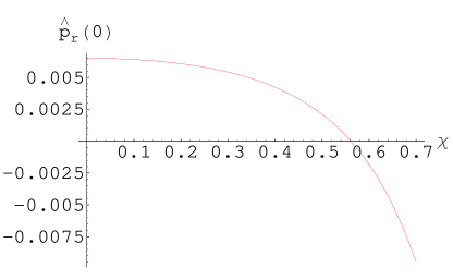
Figure 1: Variation of central density $\hat{\rho}(0)$ with $\chi$.

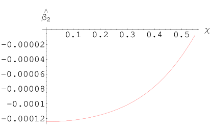
Figure 2: Variation of central pressure $\hat{p}_{r}(0)$ with $\chi$.

Figure 3: Variation of parameter $\hat{\beta}_{2}$ with $\chi$.

Figures 1 and 2 indicate that the central density $\hat{\rho}(0)$ and central pressure $\hat{p}_{r}(0)$ are monotonically decreasing with increasing values of $\chi$ for $\eta=1.147$ and $\chi\in(0,0.7]$. We see that $\hat{p}_{r}(0)>0$ only when $\chi\in[0,0.57)$, hence we take the maximum charge $\chi=0.56$ to discuss our models. Figures 3-5 show that $\hat{\beta}_{2}<0,~{}1+\hat{\gamma}_{1}>0$ and $\hat{\gamma}_{2}<0$ for the same value of $\eta$. We can have positive definite roots from Eqs.(66) and (71), hence we can analyse the models with positive matter density $\hat{\rho}(x)$. It is obvious that $\chi=0$ implies no charge. If we increase $\chi$, it increases repulsive electrostatic forces and consequently pressure and density change.

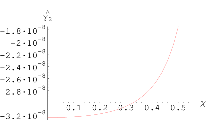
Figure 4: Variation of parameter $\hat{\gamma}_{1}$ with $\chi$.

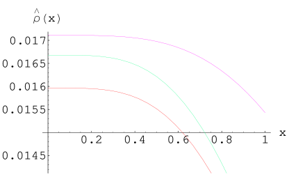
Figure 5: Variation of parameter $\hat{\gamma}_{2}$ with $\chi$.

Figure 6: Variation of matter density $\hat{\rho}(x)$ with $x$ for different values of $\chi$. Red, green and purple curves correspond to $\chi=0,0.3,0.56$ respectively.

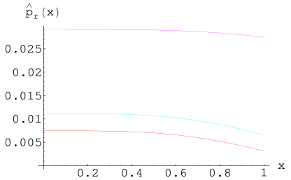
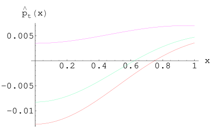
Figure 7: Variation of radial pressure $\hat{p}_{r}(x)$ with $x$ for different values of $\chi$. Red, green and purple curves correspond to $\chi=0,0.3,0.56$ respectively.

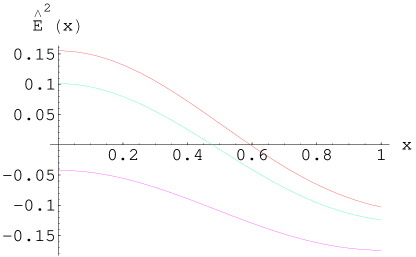
Figure 8: Variation of tangential pressure $\hat{p}_{t}(x)$ with $x$ for different values of $\chi$. Red, green and purple curves correspond to $\chi=0,0.3,0.56$ respectively.

Figure 9: Variation of Electric field intensity $\hat{E}(x)$ with $x$ for different values of $\chi$. Red, green and purple lines correspond to $\chi=0,0.3,0.56$ respectively.

Now we explore the behavior of matter sources for our models at different charges. Firstly, we investigate the sources with linear EoS. Figures 6-9 show the corresponding matter density, radial pressure, tangential pressure and electric field intensity. The graphs of density and pressure show the increasing behavior while the electric field intensity is decreasing with the increasing values of $\chi$. Further, $\hat{E}(x)$ decreases at every point in the interval $x\in(0,0.1]$ with increasing $\chi$. Figure 10 shows the behavior of charge density $\hat{\sigma}$ which is unbounded for each value of $\chi$.

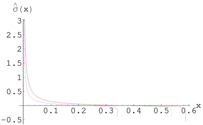
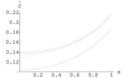
Figure 10: The charge density $\hat{\sigma}(x)$ for different values of $\chi$. Red, green and purple curves correspond to $\chi=0,0.3,0.56$ respectively.

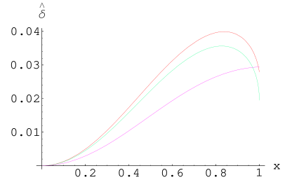
Figure 11: Measure of anisotropy $\hat{\delta}$ for the first model with $x$ for different values of $\chi$. Red, green and purple curves correspond to $\chi=0,0.3,0.56$ respectively.

Figure 12: Measure of anisotropy $\hat{\delta}$ for the second model with $x$ for different values of $\chi$. Red, green and purple lines correspond to $\chi=0,0.3,0.56$ respectively.

The analysis for models with nonlinear and Chaplygin gas EoS indicates that these models are similar to the model satisfying linear EoS. These models correspond to the decreasing matter densities and pressures. Each EoS affects the dependance of the measure of anisotropy $\hat{\delta}$ on $x$. The only difference arising from the three models is about the measure of anisotropy $\hat{\delta}=\hat{p}_{t}-\hat{p}_{r}$. Figure 11 displays the anisotropic parameter for the model corresponding to the linear EoS which is increasing with the increasing $\chi$. Figures 12 and 13 show the anisotropic parameters corresponding to the nonlinear and Chaplygin gas EoS respectively. From figures, we see that the anisotropic parameter for nonlinear EoS is increasing while for the Chaplygin gas EoS, it is decreasing with increasing $\chi$. In addition, Eq.(18) contains proper charge density $\sigma$ which implies that

$$E(r)=\frac{4\pi re^{\nu-\mu}}{r^{2}}\int_{0}^{r}r\sigma e^{2\mu-2\nu}dr=\frac{q(r)}{r^{2}},$$ (76)

where

$$q(r)=4\pi re^{\nu-\mu}\int_{0}^{r}r\sigma e^{2\mu-2\nu}dr$$ (77)

which is the net charge inside the cylinder of radius $r$.

For our cylindrically symmetric fluid models, Eqs.(7)-(10) represent the basic source parameters. We formulate table I by computing adimensional values for these basic sources. Approximate numerical values for central density $\hat{\rho}(0)$, central pressure $\hat{p}(0)$, tangential pressure $\hat{p}_{t}(1)$ and electric field intensity $\hat{E}^{2}(1)$, are shown in table I. We note that the maximum value of $\hat{\rho}(0)$ and the value of $\hat{p}_{r}(0)$ are smaller than maximum of $\hat{p}_{t}(1)$. These maxima correspond to zero net charge sources. The source variables $\hat{\rho}(0),~{}\hat{p}_{r}(0)$ with maximum charge ($\chi=0.56$) have been changed while $\hat{p}_{t}(0)$ changes its sign at the maximum charge. To compensate the stronger electric repulsion, this sign inversion of tangential pressure is necessary. This is summarized in the following table:

Table I. Approximate numerical values of some quantities.

$\chi$	$\hat{\rho}(0)$	$\hat{p}(0)$	$\hat{p}_{t}(1)$	$\hat{E}^{2}(1)$
0	0.0221364	0.00651431	0.00830257	0.266397
0.56	0.0172785	0.0000738598	-0.0000726	0.370451

Now we discuss some consequences of our results.

5.1 Stability

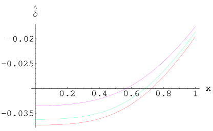
Figure 13: Measure of anisotropy $\hat{\delta}$ for the third model with $x$ for different values of $\chi$. Red, green and purple lines correspond to $\chi=0,0.3,0.56$ respectively.

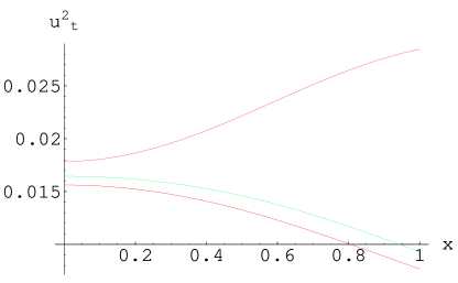
Figure 14: Variation of radial sound velocity $\hat{u}_{r}(x)$ with $x$ for different values of $\chi$. Red, green and purple lines correspond to $\chi=0,0.3,0.56$ respectively.

Figure 15: Variation of tangential sound velocity $\hat{u}_{t}(x)$ with $x$ for different values of $\chi$. Red, green and purple curves correspond to $\chi=0,0.3,0.56$ respectively.

Bertolami and Paramos [21] argued that if the generalized Chaplygin gas tends to a smooth distribution over space then most density perturbations tend to be flattened within a time scale related to their initial size and the characteristic speed of sound. One of the important physical acceptability conditions for anisotropic matter is that the squares of radial and tangential sound speeds ($u_{r}^{2}=\frac{dp_{r}}{d\rho}$ and $u_{t}^{2}=\frac{dp_{t}}{d\rho}$) should be less than the speed of light [25]. We explore it for the linear EoS model. The graphs of the squares of radial and tangential sound velocities are shown in Figures 14 and 15 respectively. These indicate that $u_{r}^{2}$ is independent of $x$ and decreases with increasing $\chi$ while $u_{t}^{2}$ monotonically increases with increasing $x$ and also increases with increasing $\chi$ for fixed $x$. For three particular values considered here, these parameters satisfy $0<u_{r}^{2}<1$ and $0<u_{t}^{2}<1$ everywhere within the charged fluid.

Now we use Herrera [25] and Andreasson’s [26] approach to identify potentially unstable or stable anisotropic matter configuration. According to their approach, $|u_{t}^{2}-u_{r}^{2}|\leq 1$ as shown in Figure 16. This implies that

$$(i)\quad-1\leq u_{t}^{2}-u_{r}^{2}\leq 0,\quad(ii)\quad 0<u_{t}^{2}-u_{r}^{2}\leq 1.$$

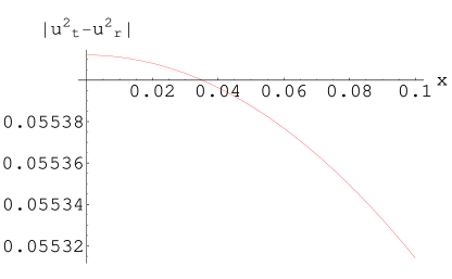
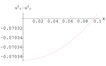
Figure 16: $|u_{t}^{2}-u_{r}^{2}|\leq 1$

Figure 17: $-1<u_{t}^{2}-u_{r}^{2}\leq 0$

The first expression corresponds to the potentially stable model which is obvious from Figure 17, while the second expression corresponds to the potentially unstable model. We note that our model satisfy the potentially stable condition. If the graph of $u_{t}^{2}-u_{r}^{2}$ keeps the same sign everywhere within a matter distribution, there will be no cracking and the system is stable. If there is a change of sign then it is alternating potentially unstable to stable region within the matter distribution and vice versa.

5.2 Energy Conditions

The energy conditions of the charged anisotropic fluid, the weak energy condition, the strong energy condition and the dominant energy condition are satisfied if and only if the following inequalities hold:

$$\hat{\rho}+\hat{p}_{r}\geq 0,$$ (78)

$$\hat{\rho}+\frac{\hat{E}^{2}}{8\pi}\geq 0,$$ (79)

$$\hat{\rho}+\hat{p}_{t}+\frac{\hat{E}^{2}}{4\pi}\geq 0,$$ (80)

$$\hat{\rho}+\hat{p}_{r}+2\hat{p}_{t}+\frac{\hat{E}^{2}}{4\pi}\geq 0,$$ (81)

$$\hat{\rho}+\frac{\hat{E}^{2}}{8\pi}-|\hat{p}_{r}-\frac{\hat{E}^{2}}{8\pi}|\geq 0,$$ (82)

$$\hat{\rho}+\frac{\hat{E}^{2}}{8\pi}-|\hat{p}_{t}+\frac{\hat{E}^{2}}{8\pi}|\geq 0.$$ (83)

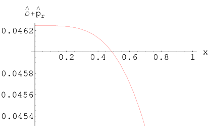
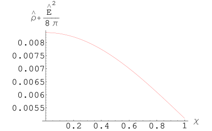
Figure 18: Weak Energy Condition 1

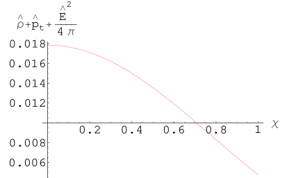
Figure 19: Weak Energy Condition 2

Figure 20: Strong Energy Condition 1

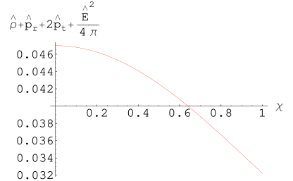
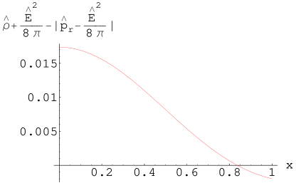
Figure 21: Strong Energy Condition 2

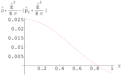
Figure 22: Dominant Energy Condition 1

Figure 23: Dominant Energy Condition 2

Figures 18-23 indicate that these inequalities hold for each $x\in[0,1]$.

5.3 The van der Waals (VDW) EoS

Lobo [19] introduced this type of bounded source for the sake of cosmology. Here we express this approach with VDW EoS given by

$$p_{r}=\frac{\omega_{1}\rho}{1-\omega_{3}\rho}-\omega_{2}\rho^{2}.$$ (84)

This is used to describe dark matter and dark energy as a single fluid. It is assumed that the interior and exterior metrics are joined and $E(0)=0=p_{r}(a)$. Further, $p_{r}$ is found at the center and boundary of the charged cylinder. Using Eqs.(84) and (30), it follows that

$$\omega_{2}\omega_{3}\rho^{3}-(\omega_{2}+\omega_{3})\rho^{2}+[1+\omega_{1}+\omega_{3}l(r)]\rho-l(r)=0,$$ (85)

where $\omega_{1}$ and $\omega_{2}$ are functions of $\rho(0),~{}\rho(a),~{}p_{r}(0)$ and $\omega_{3}$. We do not expect any interesting consequences from this equation, hence we leave it here.

5.4 Equilibrium Condition

Now we discuss the variation of the net charge corresponding to different forces compatible with equilibrium configuration for our models. In particular, when pressure gradients tend to zero and the charged fluid is more diluted, then what is the behavior of gravitational and other forces. Using Tolman-Oppenheimer-Volkov equation, we obtain

$$(\rho+p_{r})(e^{2\nu}(p_{r}-E^{2})-e^{4\nu-2\mu}\frac{\mu^{\prime}}{r})-\frac{dp_{r}}{dr}+\frac{\sigma qe^{\mu-\nu}}{r^{2}}+r(e^{2\mu+2\nu})(p_{t}-p_{r})=0.$$ (86)

This provides the equilibrium condition for the charged fluid elements subject to different forces. Here $q=q(r)$ as given in Eq.(77). In adimensional version, we can write

$$\hat{F}_{1}+\hat{F}_{2}+\hat{F}_{3}+\hat{F}_{4}=0,$$ (87)

where

$$\hat{F}_{1} = (\hat{\rho}+\hat{p}_{r})(e^{\hat{2B}x^{2}+2C}(\hat{p}_{r}-\hat{E}^{2})-2\hat{A}xe^{4\hat{B}x^{2}-2\hat{A}x^{2}+4C}),$$ (88)

$$\hat{F}_{2} = -\frac{d\hat{p}_{r}}{dx},$$ (89)

$$\hat{F}_{3} = \hat{\sigma}\hat{E}e^{x^{2}(\hat{B}-\hat{A}+C)},$$ (90)

$$\hat{F}_{4} = xe^{2x^{2}(\hat{B}-\hat{A}+2C)}(\hat{p}_{t}-\hat{p}_{r}).$$ (91)

The graphs of these forces with linear EoS at $\chi=0$ and $\chi=0.56$ are shown in Figures 24 and 25 respectively which indicate that the charge has a negligible effect on these forces, hence we obtain a static equilibrium. For $\chi=0,~{}\hat{F_{4}}$ point outwards at every $x\in(0,1]$ and $\hat{F_{2}}$ is along the $x$-axis. The electric force $\hat{F_{3}}$ acting on the fluid elements with unbounded $\hat{\sigma}$ located at $x=1$ is infinite. This is the weakest force because it changes sign at $x\approx 0.38$ and also the force $\hat{F}_{1}$ changes sign at $x\approx 0.9$ which is due to gravity. When $\chi=0.56$, the electric force is still unbounded and infinite. This unboundedness of the force $\hat{F}_{3}$ and sign inversion of the force $\hat{F}_{1}$ is essential for the configuration of our static, charged anisotropic model with linear EoS.

6 Outlook

The main purpose of this paper is to investigate the solutions of the coupled Einstein-Maxwell field equations for the static cylindrically symmetric spacetime. For this purpose, we have used charged anisotropic fluid with EoS in the light of Victor et al. [12] procedure developed for static spherically symmetric spacetime. In particular, the linear, nonlinear and Chaplygin EoS have been used. It is mentioned here that the linear EoS corresponds to the electrically charged isotropic strange quark stars on the basis of MIT bag model [27]. Our model with linear EoS also corresponds to the model by Victor et al. [12] for the charged anisotropic spherically symmetric fluid with the same EoS. We know that the nonlinear and Chaplygin EoS are used to describe non-static neutral gravitational isotropic fluids. Here we are taking static charged anisotropic fluid as we would like to explore the interior regions and the fluid vacuum interfaces of the charged anisotropic cylindrically symmetric stars with these EoS.

We have used the assumptions of Karori and Barua to explore the charged anisotropic static cylinder. Our models with nonlinear and Chaplygin EoS correspond to the dark matter and dark energy with constant matter densities and pressures [28]. Delgaty and Lake [29] proposed some physical conditions acceptable for perfect fluids, i.e., regularity of the charge at the origin, positive matter density and pressure, decreasing matter density and pressure with increasing $r$, causal sound propagation and smooth matching of internal and external metrics at boundary of the source. Burke and Hobill [30] added one more condition that sound velocity must be monotonically decreasing with increasing $r$ which was imposed on spherical perfect fluid [31, 32]. We have found that our cylindrical models satisfy most of the above physical conditions. In our case, conflict may arise for increasing tangential sound velocity, constant radial velocity and negative tangential pressure for higher values of $\chi$.

Finally, we would like point out that we have also explained charged anisotropic static cylindrically symmetric models in our recent paper [17] by using Thirukkanesh and Maharaj approach. In that paper, we have found that the charge distribution as well as $E$ become singular at $r=0$. However, here we have found non-singular behavior of these quantities.

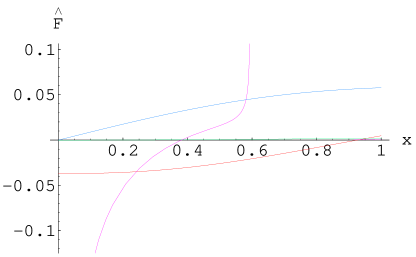
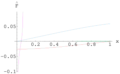
Figure 24: Four different forces $\hat{F}_{1}(x)$, $\hat{F}_{2}(x)$, $\hat{F}_{3}(x)$ and $\hat{F}_{4}(x)$ corresponding to red, green, purple and blue curves respectively are acting on the fluid elements in static equilibrium for $\chi=0$.

Figure 25: Four different forces $\hat{F}_{1}(x)$, $\hat{F}_{2}(x)$, $\hat{F}_{3}(x)$ and $\hat{F}_{4}(x)$ corresponding to red, green, purple and blue curves respectively are acting on the fluid elements in static equilibrium for $\chi=0.56$.

References

• [1] Stephani, H., Kramer, D., MacCallum, M. Hoenselaers, C. and Herlt, E.: Exact Solutions of Einstein’s Field Equations (Cambridge University Press, 2003).
• [2] Evan, A.B.: J. Phys. A10(1977)1303.
• [3] Bronnikov, K.A.: J. Phys. A12(1979)201.
• [4] Laterlier, P.S. and Tabensky, R.R.: Nuovo Cimento B28(1975)407.
• [5] Kramer, D.: Class. Quantum Grav. 5(1988)393.
• [6] Ivanov, B.V.: Phys. Rev. D65(2002)104001.
• [7] Sharma, R. and Maharaj, S.D.: Mon. Not. R. Astron. Soc. 375(2007)1265.
• [8] Bonner, B.W.: Z. Phys. 160(1960)59.
• [9] Ray et al.: Phys. Rev. D82(2010)104055.
• [10] Thirukkanesh, S. and Maharaj, S.D.: Class. Quantum Grav. 25(2008)253001.
• [11] Horvat, D., Ilijic, S. and Marunovic, A.: Class. Quantum Grav. 26(2009)025003.
• [12] Victor et al.: Phys. Rev. D82(2010)044052.
• [13] Nilsson, U., Uggla, C., and Marklund, M.: J. Math. Phys. 39(1998)3336.
• [14] Sharif, M.: J. Korean Phys. Soc. 37(2000)624.
• [15] Sharif, M. and Fatima, S. Gen. Relativ. Gravit. 43(2011)127.
• [16] Som, M.M.: Foc. Phys. Soc. 90(1967)1149.
• [17] Sharif, M. and Fatima, H.I.: Charged Anisotropic Static Cylindrically Symmetric Models, submitted for publication.
• [18] Krori, K.D. and Barua, J.: J. Phys. A Math. Gen. 8(1975)508.
• [19] Lobo, F.S.N.: Phys. Rev. D75(2006)024023.
• [20] Prasana, A.R.: Phys. Rev. D11(1975)2083.
• [21] Bertolami, O. and Paramos, J.: Phys. Rev. D72(2005)123512.
• [22] Jamil, M., Farooq, U. and Rashid, M.A.: Phys. J. C59(2009)907.
• [23] Chao-Guang, H.: Acta Physica Sinica 4(1995)617.
• [24] Junevicus, G.J.G.: J. Phys. A Math. Gen. 9(1976)2069.
• [25] Herrera, L.: Phys. Lett. A165(1992)206.
• [26] Andr easson, H.: Commun. Math. Phys. 288(2009)715.
• [27] Negreiros et al.: Phys. Rev. D80(2009)083006.
• [28] Tsujikawa, S.: Phys. Rev. D76(2007)023514.
• [29] Delgaty, M.S.R. and Lake, K.: Comput. Phys. Commun. 115(1998)395.
• [30] Burke, J. and Hobill, D.: arXiv:0910.3230.
• [31] Harko, T. and Mak, M.K.: Annalen Phys. 11(2002)3.
• [32] Abreu, H. Hernandez, H. and Nunez, L.A.: Class. Quantum Grav. 24(2007)4631.
Refer to caption