Using the de Haas-van Alphen effect to map out the closed
three-dimensional Fermi surface of natural graphite

Abstract

The Fermi surface of graphite has been mapped out using de Haas van Alphen (dHvA) measurements at low temperature with in-situ rotation. For tilt angles $\theta>60^{\circ}$ between the magnetic field and the c-axis, the majority electron and hole dHvA periods no longer follow the $\cos(\theta)$ behavior demonstrating that graphite has a 3 dimensional closed Fermi surface. The Fermi surface of graphite is accurately described by highly elongated ellipsoids. A comparison with the calculated Fermi surface suggests that the SWM trigonal warping parameter $\gamma_{3}$ is significantly larger than previously thought.

Graphite consists of Bernal stacked graphene layers with a weak inter layer coupling which leads to an in-plane dispersion which depends on the momentum in the direction perpendicular to the layers, $k_{z}$. Graphite is a semi metal with the carriers occupying a small region along the $H-K-H$ edge of the hexagonal Brillouin zone. The Slonczewski, Weiss, and McClure (SWM) Hamiltonian with its seven tight binding parameters $\gamma_{0},...,\gamma_{5},\Delta$, is based on group theoretical considerations and provides a remarkably accurate description of the band structure of graphite Slonczewski and Weiss (1958); McClure (1960). In a magnetic field, when trigonal warping is included ($\gamma_{3}\neq 0$) levels with orbital quantum number $n$ couple to levels with orbital quantum number $n+3$ and the Hamiltonian has infinite order. However, the infinite matrix can be truncated as the eigen values converge rapidly Nakao (1976). The validity of the SMW-model, has been extensively verified using many different experimental techniques e.g. Shubnikov-de Haas (SdH), de Haas-van Alphen (dHvA), thermopower, magneto-transmission, and magneto-reflectance measurements Soule (1958); Soule et al. (1964); Williamson et al. (1965); Schroeder et al. (1968); Woollam (1970, 1971a); Orlita et al. (2008); Chuang et al. (2009); Schneider et al. (2009); Zhu et al. (2009); Schneider et al. (2010a); Hubbard et al. (2011); Ubrig et al. (2011). However, recently claims Luk’yanchuk and Kopelevich (2004, 2006) for the observation, in electrical transport measurements, of massless two-dimensional (2D) charge carriers with a Dirac-like energy spectrum have caused much controversy Mikitik and Yu. V. Sharlai (2006); Luk’yanchuk and Kopelevich (2010); Schneider et al. (2010b).

The Fermi surface of graphite has electron and hole majority carrier pockets with maximal extremal cross sections at $k_{z}=0$ (electrons) $k_{z}\approx 0.35$ (holes). For both types of charge carriers the in-plane dispersion is parabolic (massive fermions). Only at the H point ($k_{z}=0.5$) the in-plane dispersion is linear, similar to that of charge carriers in graphene (massless Dirac fermions). At the H-point,there two possible extremal orbits. A minimal (neck) orbit of the majority hole carriers, which gives rise to minority carrier effects ($\alpha$-surface) and a maximal extremal orbit of the small ellipsoidal minority hole pocket ($\beta$ surface) which results from the intersection of the two majority hole ellipsoids. The existence of the three minority carrier pockets at the K-point, the so called outrigger pieces, was proposed by Nozières Nozières (1958), however their existence is considered to be unlikely due to the rather large value of $\gamma_{3}$, the SWM trigonal warping parameter, required.

In this Letter, we present a complete map of the Fermi surface of natural graphite obtained from dHvA measurements at low temperature ($T\approx 0.4$ K) with in-situ rotation. For tilt angles $\theta<60^{\circ}$, the dHvA periods of both the electrons and holes follow a $cos(\theta)$ dependence. While such a quasi-2D behavior is well established in the literature, previous dHvA measurements  Williamson et al. (1965), were unable to distinguish between a highly elongated 3D ellipsoid and a cylindrical 2D Fermi surface. Our results at larger tilt angles demonstrate unequivocally that graphite has a 3D closed Fermi surface which is accurately described by highly elongated ellipsoids provided the spin splitting is included. A comparison of our data with the full SWM calculations allows us to refine the SWM tight binding parameters, notably $\gamma_{3}$ is found to be significantly larger than previously thought.

For the dHvA measurements we used a mm-size piece of natural graphite, which was mounted on a CuBe cantilever which forms the mobile plate of a capacitive torque meter. The capacitive torque signal was measured with a lock-in amplifier using conventional phase sensitive detection at $5.3$ kHz. The measurements were performed using a $16$ T superconducting magnet and a dilution fridge, equipped with an in situ rotation stage. Fig. 1 (a) shows the torque $\tau$ as a function of the total magnetic field from $B=0-0.21$ T for a tilt angle $\theta=16^{\circ}$. The torque shows the expected dependence, $\tau(B)\propto-B^{2}$ (broken line), since $\tau=MB\sin(\theta)$ and the magnetization $M$ depends linearly on the magnetic field. Superimposed on the large monotonic background, small quantum oscillations are clearly visible, which reflect the oscillatory magnetization of the system as Landau levels pass through the Fermi energy. The dHvA oscillations can be better observed in the oscillatory torque ($\tau_{osc}$). Here the monotonic background has been removed by subtracting a smoothed (moving window average) data curve. The torque $\tau\propto sin(\theta)$ so that we cannot directly access the quantum oscillations in perpendicular field. In order to compare with our previous magnetotransport measurements we use the low angle $\theta=16^{\circ}$ data writing $B_{\perp}=B\cos(\theta)$. Fig. 1(a) shows $\tau_{osc}(B)$.

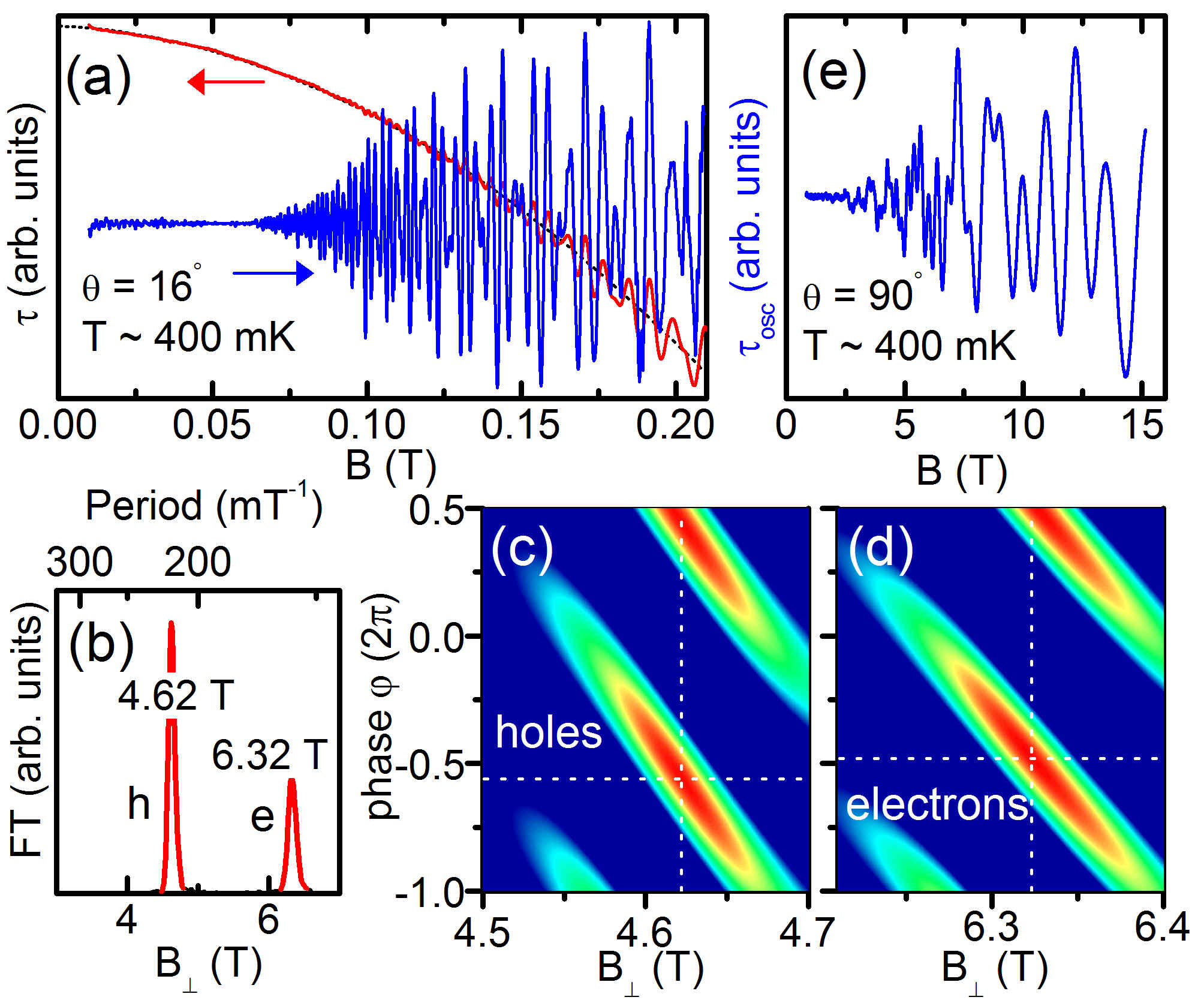
Figure 1: (color online) (a) The torque $\tau$ and oscillatory torque $\tau_{osc}$ versus total magnetic field for $\theta=16^{\circ}$. (b) Fourier transform of $\tau(1/B\cos(\theta))$. (c-d) The phase shift function $\mathrm{\Re}\left[\mathrm{exp}\left(i\varphi\right)f(\mathrm{B_{\perp}})\right]$ as a function of the phase and frequency. (e) Oscillatory torque $\tau_{osc}(B)$ for $B\parallel ab$ ($\theta=90^{\circ}$).

The phase and the frequency of the dHvA oscillations, were extracted from a Fourier analysis. The fundamental frequencies $B_{F\perp}^{e}=6.32\pm 0.1$ T and $B_{F\perp}^{h}=4.62\pm 0.1$ T for electrons and holes respectively, are obtained from the amplitude of the Fourier transform of $\tau_{osc}(1/B_{\perp})$ (see Fig. 1 (b)). In Fig. 1(c) and (d) we plot the phase shift function $K(\varphi,B_{\perp})=\mathrm{\Re}\left[\mathrm{exp}\left(i\varphi\right)f(\mathrm{B_{\perp}})\right]=\cos(\varphi-\varphi_{0})F(B_{\perp})$ as a function of the perpendicular magnetic field and the phase. The fundamental frequency and the phase $\varphi_{0}$ can be found from the maxima in the $\varphi-B$ plane. The phase values in units of $2\pi$ obtained are $\varphi_{0}^{e}=-(0.48\pm 0.1)$ and $\varphi_{0}^{h}=-(0.56\pm 0.1)$. The phase $\varphi_{0}=\gamma-\delta$ with $\gamma=1/2$ for massive Fermions or $\gamma=0$ for massless Dirac fermions. For a 3D Fermi surface the curvature along $k_{z}$ gives $\delta=\pm 1/8$ for minimum/maximum extremal cross sections. In contrast a cylindrical 2D Fermi surface gives $\delta=0$. We can therefore conclude, in agreement with recent dHvA measurements on highly oriented pyrolytic graphite (HOPG) Hubbard et al. (2011), that both the electrons and holes are massive Fermions with a parabolic energy spectrum (i.e. $\gamma=1/2$). In Fig. 1(e) we show the oscillatory torque $\tau_{osc}(B)$ in the $B\|ab$ configuration ($\theta=90^{\circ}$). The $B\parallel ab$ configuration can be found very precisely ($\delta\theta<0.1^{\circ}$), since the magnetization background changes sign at $\theta=90^{\circ}$. Well pronounced quantum oscillations are observed demonstrating unequivocally that the Fermi surface of graphite is 3D and closed.

In order to map out the Fermi surface, we have performed systematic angle dependent measurements. In Fig. 2(a) we plot the amplitude of the Fourier transform of $\tau_{osc}(1/B)$ as a function of the period of the oscillations) and the tilt angle $\theta$. The hole and electron features, together with the hole harmonic, can clearly be distinguished. For angles $\theta<60^{\circ}$, the dHvA period for both electrons and holes follow the well documented Soule et al. (1964); Williamson et al. (1965) $\cos(\theta)$ dependence. Such a behavior is characteristic of either a 2D material or very anisotropic material with an almost perfectly cylindrical Fermi surface. We can distinguish between these two scenarios at higher tilt angle. The non cylindrical nature of the Fermi surface is clearly revealed for $\theta\geq 60^{\circ}$ where deviations from the $\cos(\theta)$ behavior, are observed. Namely for $\theta\geq 75^{\circ}$ (see inset of Fig. 2), the slope of the dHvA periods for both the electrons and holes features changing dramatically reaching almost zero close to $\theta=90^{\circ}$ (see Fig. 2(b)). In addition, the hole feature clearly splits into two around $\theta=75^{\circ}$ due to a lifting of the spin degeneracy.

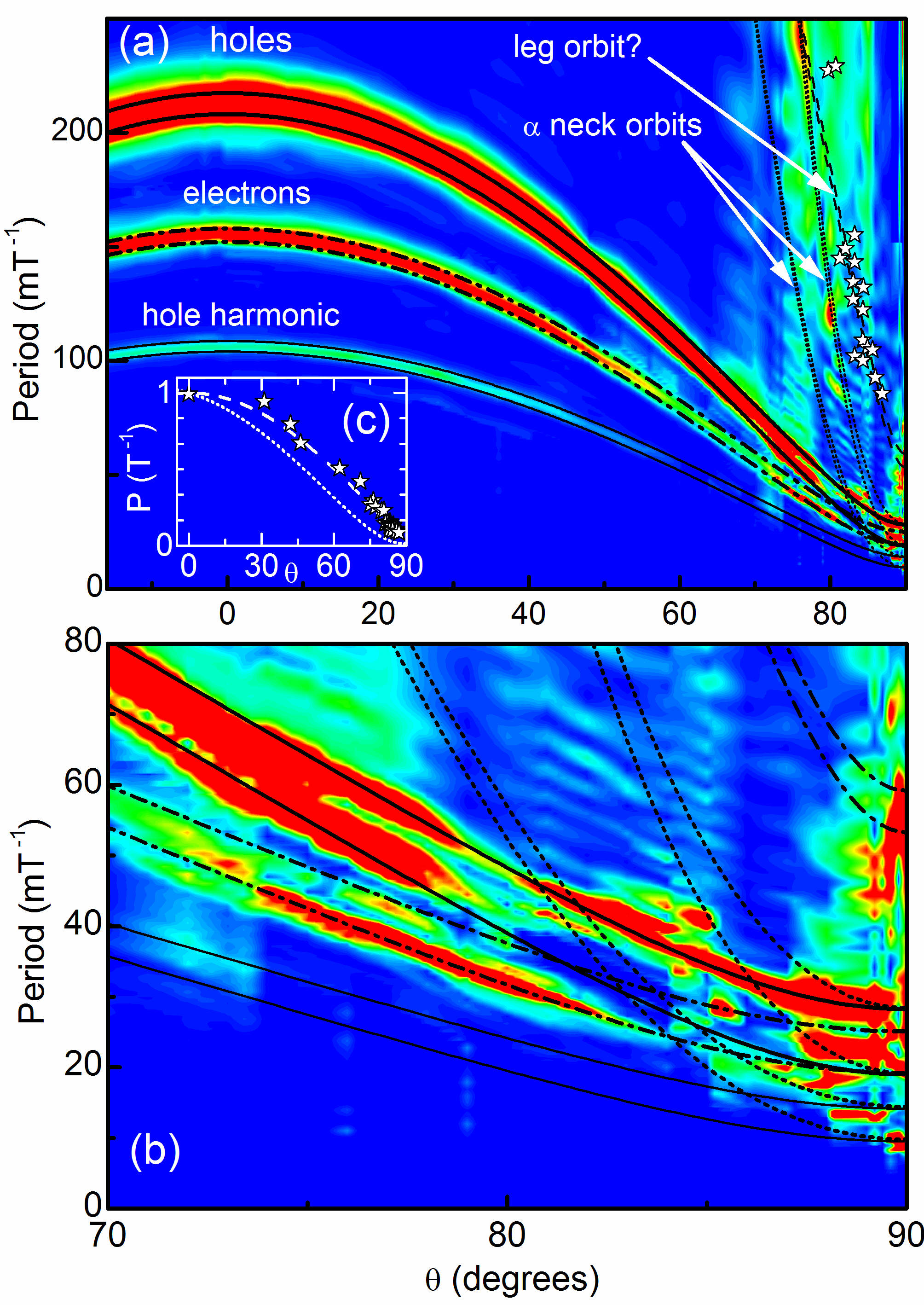
Figure 2: (color online) (a-b) Color plot : Amplitude of the Fourier transform of $\tau_{osc}(1/B)$ as a function of the period of the oscillations and the tilt angle ($\theta$). The calculated dHvA periods for ellipsoidal electron and hole Fermi surfaces are also shown for hole (solid lines), hole harmonic (thin solid lines), and electrons (dot-dash). The hole neck orbits with and without breakdown are shown as dotted lines. Woollam’s minority carrier dataWoollam (1971b) is shown as symbols. The dashed line is the prediction for an ellipsoid. (c) Woollam’s minority carrier data plotted over an extended range. The prediction for an ellipsoid (dashed line) and for a neck orbit (dotted line) are shown for comparison.

In a first approach the Fermi surface of graphite has been approximated using highly elongated ellipsoids. According to the Lifshitz-Onsager relation Onsager (1952), the fundamental frequencies $B_{F}=\hbar A/2\pi e$ are directly proportional to the extremal cross sectional areas $A$ of the Fermi surface. For the maximal extremal orbits the area is given by the intersection of a plane with the ellipse,

$$B_{F}\propto A=\pi ab/\sqrt{\sin^{2}\theta+(a^{2}/b^{2})\cos^{2}\theta},$$ (1)

where $a$ and $b$ are the semi-major and semi-minor axes of the ellipse and $\theta$ is the angle between the magnetic field and the $c$-axis of the graphite crystal. For elongated ellipsoids ($a/b\geq 5$) this follows very closely $\pi b^{2}/\cos\theta$ for $\theta<60^{\circ}$ i.e. follows closely the behavior of a 2D cylindrical Fermi surface.

For our data, matters are further complicated by the observed spin splitting for $\theta>70^{\circ}$. In order to include spin splitting in our simple model, we note that the oscillatory term can be written as,

$$\tau_{osc}\propto\cos\left(\frac{|E_{f}|}{\left(\frac{\hbar e}{m^{*}}\mp g^{*}\mu_{B}\right)B}+\phi\right)\equiv\cos\left(\frac{B_{F}^{\uparrow\downarrow}}{B}+\phi\right),$$ (2)

where $E_{f}$ is the Fermi energy, $m^{*}$ is the angle dependent effective mass, $g^{*}$ is the Landé g-factor, $\mu_{B}$ the Bohr magnetron and $\phi$ is a phase factor. From Equation 2 the frequency in the absence of spin splitting is $B_{F}=|E_{f}|m^{*}/\hbar e$. Thus, we have a simple relation between the frequency (period) of oscillations calculated for the ellipsoid and the expected frequencies when spin splitting is included,

$$1/B_{F}^{\uparrow\downarrow}=1/B_{F}\mp g^{*}\mu_{B}/2|E_{f}|$$ (3)

so that the expected splitting of the period is simply $\pm g^{*}\mu_{B}/2|E_{f}|$ independent of the angle $\theta$. The Fermi energy is $E_{F}^{h}\simeq-0.025$ eV for holes and $E_{F}^{e}=E_{f}^{h}-2\gamma_{2}\simeq 0.0246$ eV for electrons with $\gamma_{2}=-0.0243$ eV Nakao (1976). A reasonable fit to the observed splitting is obtained with $g^{*}=2.4$ for electrons and $g^{*}=4.0$ for holes. The value for holes is considerably larger than the value of $g^{*}=2.5$ found for both electrons and holes from magnetotransport Schneider et al. (2010a). It is not clear if this is due to the movement of the Fermi energy which is not taken into account in our analysis, or if $g^{*}$ is really larger for holes. The cross sectional area of the ellipsoids are obtained by fitting to the majority electron and hole frequencies at $\theta=0^{\circ}$ and at high tilt angles $\theta>70^{\circ}$. The parameters used are summarized in Table 1. The results of such a fit are plotted in Fig.2 as thick solid and dot-dash lines for the majority hole and electron pockets. The simple model fits the experimental data remarkably well, reproducing the observed angular dependence and the electron and hole spin splitting.

	$B_{f\perp}$ (T)	$A_{\perp}$	$A_{\parallel}$	$A_{\parallel}/A_{\perp}$	$A^{SWM}_{\perp}$
Maj. hole	4.7	4.49	40.3	9.0	4.33
Maj. elec.	6.45	6.15	43.1	7.0	6.26
Hole Leg(?)	$\simeq$1	0.95	17.0	17.8	-
Hole neck	$\simeq$0.43	0.41	40.3	98	0.41

Table 1: Summary of fundamental frequencies and areas of the extremal orbits (in units of $10^{12}$ cm^-2) found for the ellipsoidal and calculated SWM Fermi surface of graphite.

The minority carrier frequencies observed in graphite have been reviewed by Woollam Woollam (1971b). The area of the neck orbits can easily be calculated at the $H$-point where the dispersion $E=\hbar v_{f}\sqrt{k_{x}^{2}+k_{y}^{2}}$ is linear. The Fermi velocity $v_{f}=\sqrt{3}ea_{0}\gamma_{0}/2\hbar$ depends only on $\gamma_{0}$, whose value of $3.15$ eV is precisely known from magneto-optical data Orlita et al. (2008); Chuang et al. (2009); Ubrig et al. (2011). The area of $H$-point neck orbit for $B\perp ab$ is $\pi k_{f}^{2}=\pi E_{f}^{2}/\hbar^{2}v_{f}^{2}=0.43\times 10^{12}$ cm^-2 corresponds to a frequency of $\simeq 0.4$ T i.e., the large period ($1.2$ T^-1) minority carrier frequency of Ref. Woollam (1971b). The neck orbits have their origin in the two interpenetrating hole ellipsoids at the H-point Williamson et al. (1965). The size of this orbit is expected to increase rapidly with tilt angle as the initially small circular orbit is transformed into a large figure of eight orbit encompassing both hole ellipsoids (or a single ellipsoid if magnetic breakdown occurs at the H-point) Woollam (1971b). The area of these neck orbits, with and without magnetic breakdown, have been calculated within our simple model using the previously determined parameters for the majority hole ellipse. The only adjustable parameter is the interpenetration of the hole ellipsoids which was chosen to have the correct minority carrier frequency $\sim 0.4$ T. The calculated period of the neck orbits and are shown as dashed lines in Fig.2. The neck orbits have the same frequency the spin split majority hole and spin split majority hole harmonic at $\theta=90^{\circ}$ and so cannot be distinguished. Nevertheless, clear features correspond to the neck orbit with magnetic breakdown are observed in the data for $75<\theta<90^{\circ}$.

Woollam assigned the minority carrier period of $\simeq 1$ T^-1 to the H-point neck orbits, which in view of our results cannot be correct. Woollam’s data is plotted as symbols in Fig.2(a) and (c) and seems to join up nicely with the strong feature at around $50$ mT^-1 in our data. The calculated angular dependence for a neck orbit and an ellipsoid are shown as broken lines in Fig.2(c). Clearly, the angular dependence corresponds to an ellipsoid rather than a neck orbit. The angular dependence for an ellipsoid fitted to our data and the data of Woollam is shown in Fig.2(a).

Finally, we have calculated the SWM Fermi surface. For the diagonalization the SWM matrix is truncated to a size of $600\times 600$. The magnetic field dependence of the density of states at $E_{f}$ is calculated at $k_{z}=0$ (electrons) and $k_{z}=0.35$ (holes) assuming a reasonable Lorentzian broadening of the Landau levels. The Fourier transform is then compared with the observed frequencies for $B\perp ab$. The SWM parameters $\gamma_{0}$ and $\gamma_{1}$ are precisely known from magnetoptical dataOrlita et al. (2008); Chuang et al. (2009); Ubrig et al. (2011). $E_{f}$ and $\gamma_{3}$ are treated as fitting parameters. The hole surface is rather insensitive to $\gamma_{3}$ so that the correct hole frequency can be obtained by choosing $E_{f}$, and then the electron frequency can be tuned using $\gamma_{3}$. After a few iterations this process converges and the correct electron and hole frequencies are obtained with $E_{f}=-0.02505$ eV and $\gamma_{3}=0.443$ eV. The SWM parameters used are summarized in Table 2. The Fermi surface is then calculated by diagonalizing the SWM $4\times 4$ matrix in zero magnetic field to calculate the in plane dispersion for $k_{z}=0-0.5$ and looking for the crossing with $E_{f}$ for angles $\alpha=0-2\pi$ in the $k_{x}-k_{y}$ plane. The SWM Fermi surface is shown in Fig.3 and the calculated cross sectional areas are compared with the measured dHvA cross sections in Table 1. The good agreement confirms that the diagonalisation of the truncated $600\times 600$ matrix in magnetic field is fully consistent with the results of diagonalizing the $4\times 4$ SWM matrix in zero field.

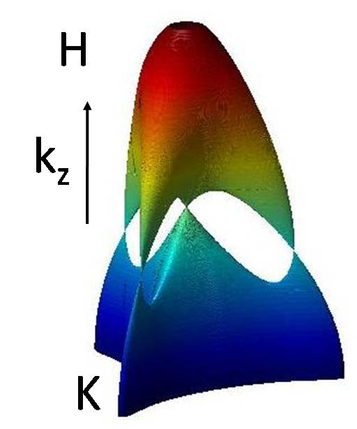
Figure 3: (color online) SWM Fermi surface of graphite along the H-K-H edge.

While the calculated Fermi surface consistent with the majority electron and hole frequencies it cannot explain the observed minority carrier frequency which is well approximated by an ellipsoid. Inspecting the SWM Fermi surface it can be seen that there is no extremal orbit in the vicinity of $\theta=0$, so that the frequency should not be observed except at high tilt angles, which is indeed the case for our data. However, this frequency is very clearly seen at $\theta=0$ in the data of Woollam. This suggests that something is missing from the calculated Fermi surface so that a significantly different set of SWM parameters might be required. Notably, increasing further the trigonal warping parameter $\gamma_{3}$ can generate minority carrier pockets.

$\gamma_{0}=3.15$ eV	$\gamma_{1}=0.375$ eV	$\gamma_{2}=-0.0243$ eV
$\gamma_{3}=0.443$ eV	$\gamma_{4}=0.07$ eV	$\gamma_{5}=0.05$ eV
$\Delta=-0.002$	$E_{f}=-0.02505$ eV

Table 2: Summary of the SWM parameters used.

In conclusion, angular dependent dHvA measurements on graphite reveal the 3D character of the Fermi surface of graphite. The Fermi surfaces are closed in all directions and well approximated by elongated ellipsoids. Spin splitting is clearly observed at high tilt angles and has to be included in the analysis in order to extract the correct Fermi surface. The SWM parameter $\gamma_{3}$ is significantly larger than previously thought.

We would like to thank Yu. I. Latyshev for providing natural graphite samples.

References

- Slonczewski and Weiss (1958) J. C. Slonczewski and P. R. Weiss, Phys. Rev. 109, 272 (1958).
- McClure (1960) J. W. McClure, Phys. Rev. 119, 606 (1960).
- Nakao (1976) K. Nakao, J. Phys. Soc. Japan 40, 761 (1976).
- Soule (1958) D. E. Soule, Phys. Rev. 112, 698 (1958).
- Soule et al. (1964) D. E. Soule, J. W. McClure, and L. B. Smith, Phys. Rev. 134, A453 (1964).
- Williamson et al. (1965) S. J. Williamson, S. Foner, and M. S. Dresselhaus, Phys. Rev. 140, A1429 (1965).
- Schroeder et al. (1968) P. R. Schroeder, M. S. Dresselhaus, and A. Javan, Phys. Rev. Lett. 20, 1292 (1968).
- Woollam (1970) J. A. Woollam, Phys. Rev. Lett. 70, 811 (1970).
- Woollam (1971a) J. A. Woollam, Phys. Rev. B 3, 1148 (1971a).
- Orlita et al. (2008) M. Orlita, C. Faugeras, G. Martinez, D. K. Maude, M. L. Sadowski, and M. Potemski, Phys. Rev. Lett. 100, 136403 (2008).
- Chuang et al. (2009) K.-C. Chuang, A. M. R. Baker, and R. J. Nicholas, Phys. Rev. B 80, 161410 (2009).
- Schneider et al. (2009) J. M. Schneider, M. Orlita, M. Potemski, and D. K. Maude, Phys. Rev. Lett. 102, 166403 (2009).
- Zhu et al. (2009) Z. Zhu, H. Yang, B. Fauqué, Y. Kopelevich, and K. Behnia, Nature Physics 6, 26 (2009).
- Schneider et al. (2010a) J. M. Schneider, N. A. Goncharuk, P. Vasek, P. Svoboda, Z. Vyborny, L. Smrcka, M. Orlita, M. Potemski, and D. K. Maude, Phys. Rev. B 81, 195204 (2010a).
- Hubbard et al. (2011) S. B. Hubbard, T. J. Kershaw, A. Usher, A. K. Savchenko, and A. Shytov, Phys. Rev. B 83, 035122 (2011).
- Ubrig et al. (2011) N. Ubrig, P. Plochocka, P. Kossacki, M. Orlita, D. K. Maude, O. Portugall, and G. L. J. A. Rikken, Phys. Rev. B 83, 073401 (2011).
- Luk’yanchuk and Kopelevich (2004) I. A. Luk’yanchuk and Y. Kopelevich, Phys. Rev. Lett. 93, 166402 (2004).
- Luk’yanchuk and Kopelevich (2006) I. A. Luk’yanchuk and Y. Kopelevich, Phys. Rev. Lett. 97, 256801 (2006).
- Mikitik and Yu. V. Sharlai (2006) G. P. Mikitik and Yu. V. Sharlai, Phys. Rev. B 73, 235112 (2006).
- Luk’yanchuk and Kopelevich (2010) I. A. Luk’yanchuk and Y. Kopelevich, Phys. Rev. Lett. 104, 119701 (2010).
- Schneider et al. (2010b) J. M. Schneider, M. Orlita, M. Potemski, and D. K. Maude, Phys. Rev. Lett. 104, 119702 (2010b).
- Nozières (1958) P. Nozières, Phys. Rev. 109, 1510 (1958).
- Woollam (1971b) J. A. Woollam, Phys. Rev. B 4, 3393 (1971b).
- Onsager (1952) L. Onsager, Phil. Mag. Ser. 7 43, 1006 (1952).