Power Allocation for Outage Minimization in Cognitive Radio Networks with Limited Feedback

Abstract

We address an optimal transmit power allocation problem that minimizes the outage probability of a secondary user (SU) who is allowed to coexist with a primary user (PU) in a narrowband spectrum sharing cognitive radio network, under a long term average transmit power constraint at the secondary transmitter (SU-TX) and an average interference power constraint at the primary receiver (PU-RX), with quantized channel state information (CSI) (including both the channels from SU-TX to SU-RX, denoted as $g_{1}$ and the channel from SU-TX to PU-RX, denoted as $g_{0}$) at the SU-TX. The optimal quantization regions in the vector channel space is shown to have a ’stepwise’ structure. With this structure, the above outage minimization problem can be explicitly formulated and solved by employing the Karush-Kuhn-Tucker (KKT) necessary optimality conditions to obtain a locally optimal quantized power codebook. A low-complexity near-optimal quantized power allocation algorithm is derived for the case of large number of feedback bits. More interestingly, we show that as the number of partition regions approaches infinity, the length of interval between any two adjacent quantization thresholds on the $g_{0}$ axis is asymptotically equal when the average interference power constraint is active. Similarly, we show that when the average interference power constraint is inactive, the ratio between any two adjacent quantization thresholds on the $g_{1}$ axis becomes asymptotically identical. Using these results, an explicit expression for the asymptotic SU outage probability at high rate quantization (as the number of feedback bits goes to infinity) is also provided, and is shown to approximate the optimal outage behavior extremely well for large number of bits of feedback via numerical simulations. Numerical results also illustrate that with 6 bits of feedback, the derived algorithms provide SU outage performance very close to that with full CSI at the SU-TX.

I Introduction

Scarcity of available vacant spectrum is limiting the growth of wireless products and services [3]. Traditional spectrum licensing policy forbids unlicensed users to transmit in order to avoid unfavorable interference at the cost of spectral utilization efficiency. This led to the idea of cognitive radio (CR) technology, originally introduced by J. Mitola [4], which holds tremendous promise to dramatically improve the efficiency of spectral utilization.
The key idea behind CR is that an unlicensed/secondary user (SU) is allowed to communicate over a frequency band originally licensed to a primary user (PU), as long as the transmission of SU does not generate unfavorable impact on the operation of PU in that band. Effectively, three categories of CR network paradigms have been proposed: interweave, overlay, and underlay [5]. In the underlay systems, also known as spectrum sharing model, which is the focus of this paper, the SU can transmit even when the PU is present, but the transmitted power of SU should be controlled properly so as to ensure that the resulting interference does not degrade the received signal quality of PU to an undesirable level [6] by imposing the so called interference temperature [7] constraints at PU (average or peak interference power (AIP/PIP) constraint) and as well as to enhance the performance of SU transmitter (SU-TX) to SU receiver (SU-RX) link.
Various notions of capacity for wireless channels include ergodic capacity (for delay-insensitive services), delay-limited capacity and outage probability (for real-time applications). These information theoretic capacity notions constitute important performance measures in analyzing the performance limits of CR systems. In [7], the authors investigated the ergodic capacity of such a dynamic narrowband spectrum sharing model under either AIP or PIP constraint at PU receiver (PU-RX) in various fading environments. The authors of [8] extended the work in [7] to asymmetric fading environments. In [9], the authors studied optimum power allocation for three different capacity notions under both AIP and PIP constraints. In [6], the authors also considered the transmit power constraint at the SU-TX and investigated the optimal power allocation strategies to achieve the ergodic capacity and outage capacity of SU under various combinations of secondary transmit (peak/average) power constraints and interference (peak/average) constraints.
Achieving the optimal system performance requires the SU-TX to acquire full channel state information (CSI) including the channel information from SU-TX to PU-RX and the channel information from SU-TX to SU-RX. Most of the above results assume perfect knowledge or full CSI, which is very difficult to implement in practice, especially the channel information from SU-TX to PU-RX without PU’s cooperation. A few recent papers have emerged that address this concern by investigating performance analysis with various forms of partial CSI at SU-TX, such as noisy CSI and quantized CSI. With assumption of perfect knowledge of the CSI from SU-TX to SU-RX channel, [10] studied the effect of imperfect channel information of the SU-TX to PU-RX channel under AIP or PIP constraint by considering the channel information from SU-TX to the PU-RX as a noisy estimate of the true CSI and employing the so-called ’tifr’ transmission policy. Another recent work [11] also considered imperfect CSI of the SU-TX to PU-RX channel in the form of noisy channel estimate (a range from near-perfect to seriously flawed estimates) and studied the effect of using a midrise uniformly quantized CSI of the SU-TX to PU-RX channel, while also assumed the SU-TX had full knowledge of the CSI from SU-TX to SU-RX channel. Recently, [12] has proposed a practical design paradigm for cognitive beamforming based on finite-rate cooperative feedback from the PU-RX to the SU-TX and cooperative feedforward from the SU-TX to the PU-RX. A robust cognitive beamforming scheme was also analyzed in [13], where full channel information on SU-TX to SU-RX channel was assumed, and the imperfect channel information on the SU-TX to PU-RX channel was modelled using an uncertainty set. Finally, [14] studied the issue of channel quantization for resource allocation via the framework of utility maximization in OFDMA based CR networks, but did not investigate the joint channel partitioning and rate/power codebook design problem. The absence of a rigorous and systematic design methodology for quantized resource allocation algorithms in the context of cognitive radio networks motivated our earlier work [15], where we addressed an SU ergodic capacity maximization problem in a wideband spectrum sharing scenario with quantized information about the vector channel space involving the SU-TX to SU-RX channel and the SU-TX to PU-RX channel over all bands, under an average transmit power constraint at the SU-TX and an average interference constraint at the PU-RX. A slightly different approach was taken in [16, 17] where the SU overheard the PU feedback link information and used this to obtain information about whether or not the PU is in outage and how the SU-TX should control its power to minimize interference on the PU-RX.
In this paper, we address the problem of minimizing the SU outage probability under an average transmit power (ATP) constraint at the SU-TX and an average interference power (AIP) constraint at the PU-RX. Similar to [15], we consider an infrastructure-based narrowband spectrum sharing scenario where a SU communicates to its base station (SU-BS) on a narrowband channel shared with a PU communicating to its receiver PU-RX contained within the primary base station (PU-BS). The key problem is the jointly designing the optimal partition regions of the vector channel space (consisting of the SU-TX to SU-RX channel (denoted by power gain $g_{1}$) and the interfering channel between the SU-TX and PU-RX (denoted by power gain $g_{0}$)) and the corresponding optimal power codebook, and is solved offline at a central controller called the CR network manager as in [15], based on the channel statistics. The CR network manager is assumed to be able to obtain the full CSI information of the vector channel space $(g_{1},g_{0})$ in real-time from the SU-BS and PU-BS, respectively, possibly via wired links (similar to backhaul links in multicell MIMO networks connecting multiple base stations). This real-time channel realization is then assigned to the optimal channel partition and the corresponding partition index is sent to the SU-TX (and to the SU-RX for decoding purposes) via a finite-rate feedback link. The SU-TX then uses the power codebook element associated with this index for data transmission. It was shown in [15] that without the presence of the CR network manager, and thus without the ability to jointly quantize the combined channel space, the SU capacity performance is significantly degraded if one carries out separate quantization of $g_{1}$ and $g_{0}$. Even if such a CR network manager cannot be implemented in practical cognitive radio networks due to resource constraints, the results derived in this paper will serve as a valuable benchmark. Under these networking assumptions, we prove a ’stepwise’ structure of the optimal channel partition regions, which helps us explicitly formulate the outage minimization problem and solve it using the corresponding Karush-Kuhn-Tucker (KKT) necessary optimality conditions. As the number of feedback bits go to infinity, we show that the power level for the last region approaches zero, allowing us to derive a useful low-complexity suboptimal quantized power allocation algorithm called ’ZPiORA’ for high rate quantization. We also derive some other useful properties related to the channel quantizer structure as the number of feedback bits approaches infinity: (a) under an active AIP constraint, the length of interval between any two adjacent quantization thresholds on $g_{0}$ axis is asymptotically the same, and (b) while when the AIP is inactive, the ratio between any two adjacent quantization thresholds on $g_{1}$ axis asymptotically becomes identical. Finally, with these properties, we derive explicit expressions for asymptotic (as the number of feedback bits increase) behavior of the SU outage probability with quantized power allocation for large resolution quantization. Numerical studies illustrate that with only 6 bits of feedback, the designed optimal algorithms provide secondary outage probability very close to that achieved by full CSI. With 2-4 bits of feedback, ZPiORA provides a comparable performance, thus making it an attractive choice for large number of feedback bits case. Numerical studies also show that ZPiORA performs better than two other suboptimal algorithms constructed using existing approximations in the literature. Finally, it is also shown that the derived asymptotic outage behavior approximates the optimal outage extremely well as the number of feedback bits becomes large.
This paper is organized as follows. Section II introduces the system model and the problem formulation based on the full CSI assumption. Section III presents the joint design of the optimal channel partition regions and an optimal power codebook algorithm. A low-complexity suboptimal quantized power allocation strategy is also derived using novel interesting properties of the quantizer structure and optimal quantized power codebooks. In Section IV, the asymptotic behavior of SU outage probability for high resolution quantization is investigated. Simulation results are given in Section V, followed by concluding remarks in Section VI.

II System Model and Problem Formulation

We consider an infrastructure-based spectrum sharing network where a SU communication uplink to the SU-BS coexists with a PU link (to the PU-BS) within a narrowband channel. Regardless of the on/off status of PU, the SU is allowed to access the band which is originally allocated to PU, so long as the impact of the transmission of SU does not reduce the received signal quality of PU below a prescribed level. All channels here are assumed to be Rayleigh block fading channels. Let $g_{1}=|h_{1}|^{2}$ and $g_{0}=|h_{0}|^{2}$, denote the nonnegative real-valued instantaneous channel power gains for the links from SU-TX to SU-RX and SU-TX to PU-RX respectively (where $h_{1}$ and $h_{0}$ are corresponding complex zero-mean circularly symmetric channel amplitude gains). The exponentially distributed channel power gain $g_{1}$ and $g_{0}$, are statistically mutually independent and, without loss of generality (w.l.o.g), are assumed to have unity mean. The additive noises for each channel are independent Gaussian random variables with, w.l.o.g, zero mean and unit variance. For analytical simplicity, the interference from the primary transmitter (PU-TX) to SU-RX is neglected following previous work such as [6, 7](in the case where the interference caused by the PU-TX at the SU-RX is significant, the SU outage probability results derived in this paper can be taken as lower bounds on the actual outage under primary-induced interference). This assumption is justified when either the SU is outside PU’s transmission range or the SU-RX is equipped with interference cancellation capability particularly when the PU signal is strong.
Given a channel realization (${g}_{0},g_{1}$), let the instantaneous transmit power (with full CSI) at the SU-TX be represented by $p({g}_{0},g_{1})$, then the maximum mutual information of the SU for this narrowband spectrum sharing system can be expressed as $R(g_{1},p({g}_{0},g_{1}))=\frac{1}{2}\log(1+g_{1}p({g}_{0},g_{1}))$, where $\log$ represents the natural logarithm. The outage probability of SU-TX with a pre-specified transmission rate $r_{0}$, is given as, $P_{out}=Pr\{R(g_{1},p({g}_{0},g_{1}))<r_{0}\}$, where $Pr\{A\}$ indicates the probability of event $A$ occurring. Using the interference temperature concept in [7], a common way to protect PU’s received signal quality is by imposing either an average or a peak interference power (AIP/PIP) constraint at the PU-RX. In [18], it was demonstrated that the AIP constraint is more flexible and favorable than the PIP constraint in the context of transmission over fading channels. Let $Q_{av}$ denotes the average interference power limit tolerated by PU-RX, then the AIP constraint can be written as, $E[g_{0}p({g}_{0},{g}_{1})]\leq Q_{av}$.
The following optimal power allocation problem that minimizes the outage probability of SU in a narrowband spectrum sharing with one PU, under both a long term average transmit power (ATP) constraint at SU-TX and an AIP constraint at the PU-RX, was considered in [6]

$$\min_{p({g}_{0},g_{1})\geq 0}~{}~{}Pr\{\frac{1}{2}\log(1+g_{1}p({g}_{0},g_{1}))<r_{0}\}$$

$$~{}~{}~{}~{}s.t.~{}~{}~{}~{}~{}E[p({g}_{0},{g}_{1})]\leq P_{av},~{}~{}~{}~{}~{}E[g_{0}p({g}_{0},{g}_{1})]\leq Q_{av}$$ (1)

where $P_{av}$ is the maximum average transmit power at SU-TX.
With the assumption that perfect CSI of both $g_{0}$ and $g_{1}$ is available at the SU-TX, the optimal power allocation scheme for Problem (1) is given by [6]: $p^{*}({g}_{0},{g}_{1})=\frac{c}{g_{1}}$ when $\lambda^{*}_{f}+\mu^{*}_{f}g_{0}<\frac{g_{1}}{c}$, and $0$ otherwise, where $c=e^{2r_{0}}-1$, and $\lambda^{*}_{f}$, $\mu^{*}_{f}$ are the optimal nonnegative Lagrange multipliers associated with the ATP constraint and the AIP constraint, respectively, which can be obtained by solving $\lambda^{*}_{f}(E[p({g}_{0},{g}_{1})]-P_{av})=0$ and $\mu^{*}_{f}(E[g_{0}p({g}_{0},{g}_{1})]-Q_{av})=0$ .
However, the assumption of full CSI at the SU-TX (especially that of ${g}_{0}$) is usually unrealistic and difficult to implement in practical systems, especially when this channel is not time-division duplex (TDD). In the next section, we are therefore interested in designing a power allocation strategy of the outage probability minimization Problem (1) based on quantized CSI at the SU-TX acquired via a no-delay and error-free feedback link with limited rate.

III Optimum Quantized power allocation (QPA) with imperfect $g_{1}$ and ${g}_{0}$ at SU-TX

III-A Optimal QPA with limited rate feedback strategy

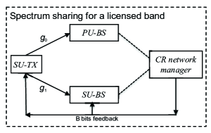
Figure 1: System model for narrowband spectrum sharing scenario with limited rate feedback

As shown in Fig.1, following our earlier work [15], we assume that there is a central controller termed as CR network manager who can obtain perfect information of ${g}_{0}$ and $g_{1}$, from PU-RX at the PU base station and SU-RX at the SU base station respectively, possibly over fibre-optic links, and then forward some appropriately quantized $(g_{0},g_{1})$ information to SU-TX through a finite-rate feedback link. For further details on the justification of resulting benefits due this assumption, see [15]. Under such a network modelling assumption, given B bits of feedback, a power codebook ${\cal{P}}$$=\{{p}_{1},\dots,{p}_{L}\}$ of cardinality $L=2^{B}$, is designed offline purely on the basis of the statistics of $g_{0}$ and $g_{1}$ information at the CR network manager. This codebook is also known a priori by both SU-TX and SU-RX for decoding purposes. Given a channel realization $({g}_{0},g_{1})$, the CR network manager employs a deterministic mapping from the current instantaneous $(g_{0},g_{1})$ information to one of $L$ integer indices (let ${\cal{I}}(g_{0},g_{1})$ denote the mapping, which partitions the vector space of $(g_{0},g_{1})$ into $L$ regions $\cal{R}$${}_{1},\dots,$$\cal{R}$_L, defined as ${\cal{I}}(g_{0},g_{1})=j,~{}~{}\text{if}~{}~{}(g_{0},g_{1})\in{\cal{R}}_{j},~{}~{}j=1,\dots,L$), and then sends the corresponding index $j={\cal{I}}(g_{0},g_{1})$ to the SU-TX (and the SU-RX) via the feedback link. The SU-TX then uses the associated power codebook element (e.g., if the feedback signal is $j$, then $p_{j}$ will be used as the transmission power) to adapt its transmission strategy.

Remark 1

Note that the CR network manager could be assumed to be located at the SU-BS for the current setup and in this case, the PU-BS simply has to cooperate with the SU-BS by sending the real-time full CSI information of $g_{0}$. However, for future generalization of our work to a multi-cell cognitive network scenario, we assume that the CR network manager is a separate entity, which can obtain information from multiple PU-BS and SU-BS if necessary.

Define an indicator function $X_{j},~{}j=1,\dots,L,$ as $X_{j}=1$ if $\frac{1}{2}\log(1+g_{1}p_{j})<r_{0}$, and $0$ otherwise. Let $Pr({\cal{R}}_{j})$, $E[\bullet|{\cal{R}}_{j}]$ represent $Pr((g_{0},g_{1})\in{\cal{R}}_{j})$ and $E[\bullet|(g_{0},g_{1})\in{\cal{R}}_{j}]$, respectively. Then the SU outage probability minimization problem with limited feedback can be formulated as

$$\min_{p_{j}\geq 0,~{}{\cal{R}}_{j}~{}\forall j}~{}\sum^{L}_{j=1}E[X_{j}|{\cal{R}}_{j}]Pr({\cal{R}}_{j})$$

$$~{}~{}s.t.~{}~{}~{}~{}~{}~{}~{}~{}~{}\sum^{L}_{j=1}E[p_{j}|{\cal{R}}_{j}]Pr({\cal{R}}_{j})\leq P_{av},~{}~{}~{}~{}~{}~{}~{}\sum^{L}_{j=1}E[g_{0}p_{j}|{\cal{R}}_{j}]Pr({\cal{R}}_{j})\leq Q_{av}.$$ (2)

Thus the key problem to solve here is the joint optimization of the channel partition regions and the power codebook such that the outage probability of SU is minimized under the above constraints.
The dual problem of (2) is expressed as, $\max_{\lambda\geq 0,~{}\mu\geq 0}~{}g(\lambda,\mu)-\lambda P_{av}-\mu Q_{av}$, where $\lambda,\mu$ are the nonnegative Lagrange multipliers associated with the ATP and AIP constraints in Problem (2), and the Lagrange dual function $g(\lambda,\mu)$ is defined as

$$g(\lambda,\mu)=\min_{{p}_{j}\geq 0,~{}{\cal{R}}_{j},~{}\forall j}~{}\sum_{j=1}^{L}E[X_{j}+(\lambda+\mu g_{0})p_{j}|{\cal{R}}_{j}]Pr({\cal{R}}_{j})$$ (3)

The procedure we use to solve the above dual problem is:

1. With fixed values of $\lambda$ and $\mu$, find the optimal solution (power codebook and quantization regions) for the Lagrange dual function (3).

2. Find the optimal $\lambda$ and $\mu$ by solving the dual problem using subgradient search method, i.e, updating $\lambda,~{}\mu$ until convergence using

   $$\lambda^{l+1}=[\lambda^{l}-\alpha^{l}(P_{av}-\sum^{L}_{j=1}E[p_{j}|{\cal{R}}_{j}]Pr({\cal{R}}_{j}))]^{+},$$

   $$\mu^{l+1}=[\mu^{l}-\beta^{l}(Q_{av}-\sum^{L}_{j=1}E[g_{0}p_{j}|{\cal{R}}_{j}]Pr({\cal{R}}_{j}))]^{+},$$ (4)

   where $l$ is the iteration number, $\alpha^{l}$, $\beta^{l}$ are positive scalar step sizes for the $l$-th iteration satisfying $\sum_{l=1}^{\infty}\alpha_{l}=\infty,\;\sum_{l=1}^{\infty}(\alpha_{l})^{2}<\infty$ and similarly for $\beta_{l}$, and $[x]^{+}=\max(x,0)$.

Remark 2

A general method to solve Step 1 is to employ a simulation-based optimization algorithm called Simultaneous Perturbation Stochastic Approximation (SPSA) algorithm (for a step-by-step guide to implementation of SPSA, see [19]), where one can use the objective function of Problem (3) as the loss function and the optimal power codebook elements for each channel partition are obtained via a randomized stochastic gradient search technique. Note that due to the presence of the indicator function and no explicit expression being available for the outage probability with quantized power allocation, we can’t directly exploit the Generalized Lloyd Algorithm (GLA) with a Lagrangian distortion, as we used in [15], to solve Problem (3). SPSA uses a simulation-based method to compute the loss function and then estimates the gradient from a number of loss function values computed by randomly perturbing the power codebook. Note that SPSA results in a local minimum (similar to GLA), but is computationally highly complex and the convergence time is also quite long.

Due to the high computational complexity of SPSA and its long convergence time to solve Problem (3), we will next derive a low-complexity approach for solving Problem (3). However, due to the original problem (2) not being convex with respect to the power codebook elements, the optimal solution we can obtain is also locally optimal.
Let ${\cal{P}}=\{p_{1},\dots,p_{L}\}$, where $p_{1}>\dots>p_{L}\geq 0$, and the corresponding channel partitioning ${\cal{R}}_{1},\dots,{\cal{R}}_{L}$ denote an optimal solution to Problem (3). Let $p({\cal I}(g_{0},g_{1}))$ represent the mapping from instantaneous $(g_{0},g_{1})$ information to the allocated power level. We can then obtain the following result:

Lemma 1

Let $\{v_{1},\dots,v_{L}\}$ denote the optimum quantization thresholds on the $g_{1}$ axis ($0<v_{1}<\dots<v_{L}$) and $\{s_{1},\dots,s_{L-1}\}$ indicate the optimum quantization thresholds on the $g_{0}$ axis ($0<s_{1}<\dots<s_{L-1}$). Then we have $\forall j,j=1,\dots,L-1$, $p({\cal{I}}(g_{0},g_{1}))=p_{j}$, if $v_{j}\leq g_{1}<v_{j+1},0\leq g_{0}<s_{j}$ and $p_{L}$ otherwise, where $v_{j}=\frac{c}{p_{j}},j=1,\dots,L$, and for $\forall j,j=1,\dots,L-1$, when $\mu>0,~{}s_{j}=\frac{1}{\mu(p_{j}-p_{L})}-\frac{\lambda}{\mu}$, while when $\mu=0,~{}s_{j}=\infty$, then condition $0\leq g_{0}<s_{j}$ boils down to $\lambda<\frac{1}{p_{j}-p_{L}}$. The region ${\cal{R}}_{L}$ includes two parts : the set ${\cal{R}}_{L1}=\{(g_{0},g_{1}):v_{j}\leq g_{1}<v_{j+1},g_{0}\geq s_{j},\forall j=0,\dots,L-1\}$ with $s_{0}=0,v_{0}=0$ and the set ${\cal{R}}_{L2}=\{(g_{0},g_{1}):g_{1}\geq v_{L},g_{0}\geq 0\}$. The entire set ${\cal{R}}_{L1}$ is in outage.

Proof: See Appendix -A.

Remark 3

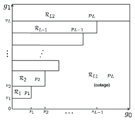
Figure 2: The ’stepwise structure’ of optimum quantization regions for $\mu>0$ case

When $\mu>0$, which implies that the AIP constraint is active, from Lemma 1, the optimum partition regions possess a stepwise structure, as shown in Fig.2. When $\mu=0$, i.e, the AIP constraint is inactive and only ATP constraint is active (we must have $\lambda>0$), Problem (2) becomes a scalar quantization problem involving quantizing $g_{1}$ only, and Lemma 1 reduces to : $p({\cal I}(g_{1}))=p_{j}$, if $v_{j}\leq g_{1}<v_{j+1},\forall j,j=1,\dots,L-1$, and $p_{L}$ otherwise, where $\lambda<\frac{1}{p_{j}-p_{L}},\forall j=1,2,\ldots,L-1$ and the two sub-regions of ${\cal{R}}_{L}$ become ${\cal{R}}_{L1}=\{g_{1}:0\leq g_{1}<v_{1}\}$ and ${\cal{R}}_{L2}=\{g_{1}:g_{1}\geq v_{L}\}$, and ${\cal{R}}_{L1}$ is in outage. Note that in this case we must have $Q_{av}\geq P_{av}$, due to $Q_{av}\geq\sum^{L}_{j=1}E[g_{0}p_{j}|{\cal{R}}_{j}]Pr({\cal{R}}_{j})=\sum^{L}_{j=1}E[p_{j}|{\cal{R}}_{j}]Pr({\cal{R}}_{j})=P_{av}$, where the last equality follows from the fact the $E[g_{0}|{\cal R}_{j}]=E[g_{0}]=1$ since ${\cal{R}}_{j}$ is formed purely based on the values of $g_{1}$, which is independent of $g_{0}$. Note also that one can easily prove the converse, that when $Q_{av}\geq P_{av}$, one must have $\mu=0$.

From Lemma 1, (due to the fading channels being independently exponentially distributed with unity mean) Problem (2) becomes,

$$\min_{p_{j}\geq 0,~{}\forall j}~{}P^{L}_{out}=1-e^{-v_{1}}+\sum^{L-1}_{j=1}(e^{-v_{j}}-e^{-v_{j+1}})e^{-s_{j}}\$$

$$~{}~{}s.t.~{}~{}p_{L}+\sum^{L-1}_{j=1}(p_{j}-p_{L})(e^{-v_{j}}-e^{-v_{j+1}})(1-e^{-s_{j}})\leq P_{av}$$

$$~{}~{}~{}~{}~{}~{}~{}~{}p_{L}+\sum^{L-1}_{j=1}(p_{j}-p_{L})(e^{-v_{j}}-e^{-v_{j+1}})(1-e^{-s_{j}}(1+s_{j}))\leq Q_{av}$$ (5)

where $P^{L}_{out}$ denotes the outage probability with $B=\log_{2}L$ bits feedback QPA, $v_{j}=\frac{c}{p_{j}},j=1,\dots,L$ and for $\forall j,j=1,\dots,L-1$, when $\mu>0,~{}s_{j}=\frac{1}{\mu(p_{j}-p_{L})}-\frac{\lambda}{\mu}$, whereas when $\mu=0,~{}s_{j}=\infty$. Although the above optimization problem may be verified to be non-convex, we can employ the KKT necessary conditions to find a local minimum for Problem (5). Taking the partial derivative of first order of the Lagrangian of Problem (5) over $p_{j},j=1,\dots,L-1$, and setting it to zero, we can obtain

$$(e^{-v_{j}}-e^{-v_{j+1}})[\lambda(1-e^{-s_{j}})+\mu(1-e^{-s_{j}}(1+s_{j}))]=e^{-v_{j}}\frac{c}{p^{2}_{j}}[\hat{f}(p_{j-1})-\hat{f}(p_{j})],~{}~{}1\leq j\leq L-1;$$ (6)

where $\hat{f}(p_{0})=1$ and $\hat{f}(p_{j})=(p_{j}-p_{L})(\lambda+\mu(1-e^{-s_{j}})),~{}1\leq j\leq L-1$. (6) also can be rewritten as $j=1,\dots,L-1$,

$$p_{j+1}=\frac{c}{v_{j}-\ln(1-\frac{\frac{c}{p^{2}_{j}}[\hat{f}(p_{j-1})-\hat{f}(p_{j})]}{\lambda(1-e^{-s_{j}})+\mu(1-e^{-s_{j}}(1+s_{j}))})},$$ (7)

Equating the partial derivative of the Lagrangian function of Problem (5) over $p_{L}$ to zero gives,

$$\sum^{L-1}_{j=1}(e^{-v_{j}}-e^{-v_{j+1}})[\lambda(1-e^{-s_{j}})+\mu(1-e^{-s_{j}}(1+s_{j}))]+e^{-v_{L}}\frac{c}{p^{2}_{L}}\hat{f}(p_{L-1})=\lambda+\mu.$$ (8)

Optimal values of $\lambda$ and $\mu$ can be determined by solving

$$\lambda[p_{L}+\sum^{L-1}_{j=1}(p_{j}-p_{L})(e^{-v_{j}}-e^{-v_{j+1}})(1-e^{-s_{j}})-P_{av}]=0$$

$$\mu[p_{L}+\sum^{L-1}_{j=1}(p_{j}-p_{L})(e^{-v_{j}}-e^{-v_{j+1}})(1-e^{-s_{j}}(1+s_{j}))-Q_{av}]=0$$ (9)

Thus, for fixed values $\lambda$ and $\mu$, we need to solve the $L$ equations given by (7), (8) to obtain the power codebook. Given $p_{1}$ and $p_{L}$, from (7) we can successively compute $p_{2},\dots,p_{L-1}$, and then we can jointly solve the equation (7) with $j=L-1$ and equation (8) numerically for $p_{1}$ and $p_{L}$. The optimal value of $\lambda$ and $\mu$ can be obtained by solving (9) with a subgradient method, i,e. by updating $\lambda$ and $\mu$ until convergence using (4). One can thus repeat the above two steps (i.e, given $\lambda$ and $\mu$ find the optimal power levels, and then using the resulting optimal power levels update $\lambda$ and $\mu$) iteratively until a satisfactory convergence criterion is met. This procedure can be formally summarized as:

1. First, if $P_{av}\leq Q_{av}$, we must have $\mu=0,~{}\lambda>0$. Starting with an arbitrary positive initial value for $\lambda$, solve (6), (8) to obtain a power codebook $\{p_{1},\dots,p_{L}\}$, and then use this codebook to update $\lambda$ by (4). Repeat these steps until convergence and the final codebook will be an optimal power codebook for Problem (5).

2. If $P_{av}>Q_{av}$, we must have $\mu>0$ by contradiction (since if $\mu=0$, we must have $P_{av}\leq Q_{av}$). Let $\lambda=0$, then solving KKT conditions gives an optimal value of $\mu$ and corresponding power codebook $\{p_{1},\dots,p_{L}\}$. With this codebook, if $\sum^{L}_{j=1}E[p_{j}|{\cal{R}}_{j}]Pr({\cal{R}}_{j})\leq P_{av}$, then it is an optimal power codebook for Problem (5). Otherwise we must have $\lambda>0$ too, in which case, starting with arbitrary positive initial values for $\lambda$ and $\mu$, obtain the corresponding power codebook $\{p_{1},\dots,p_{L}\}$, and then update $\lambda$ and $\mu$ by (4). Repeat these steps until convergence and the final codebook will be an optimal power codebook for Problem (5).

III-B Suboptimal QPA Algorithm

When the number of feedback bits $B$ (or alternatively, $L$) goes to infinity, we can obtain the following Lemma that allows us to obtain a suboptimal but computationally efficient quantized power allocation algorithm for large but finite $L$.

Lemma 2

$\lim_{L\rightarrow\infty}p_{L}=0$

Proof: See appendix -B.

Remark 4

Lemma 2 shows that regardless of whether $\mu>0$ or $\mu=0$, with high rate quantization, the power level for the last region ${\cal{R_{L}}}$ approaches zero, which also implies the following as $L\rightarrow\infty$:
1) The non-outage part of ${\cal{R_{L}}}$, given by ${\cal{R_{L}}}_{2}$, disappears gradually. In other words, ${\cal{R_{L}}}\rightarrow{\cal{R_{L}}}_{1}$. Thus, when $L\rightarrow\infty$, ${\cal{R_{L}}}$ becomes the outage region with zero power assigned to it.
2) When $\mu>0$, the quantization thresholds on the $g_{0}$ axis $s_{j}\rightarrow s_{j}^{\prime}$ (where $s_{j}^{\prime}=\frac{1}{\mu p_{j}}-\frac{\lambda}{\mu}$), which gives $v_{j}=c\lambda+c\mu s^{\prime}_{j}$, and it means all the points given by coordinates $(s^{\prime}_{j},v_{j})$ lie on the line of $g_{1}=c\lambda+c\mu g_{0}$. Therefore, as $L\rightarrow\infty$, the stepwise shape of the structure in $\mu>0$ case (i.e, the boundary between non-outage and outage regions) approaches the straight line $g_{1}=c\lambda+c\mu g_{0}$, which is consistent with the full CSI-based power allocation result in [6].

Thus, when $L$ is large, applying Lemma 2 (i.e, $p_{L}\rightarrow 0$) to Problem (5), the above $L$ KKT conditions (6) and (8) can be simplified into $L-1$ equations:

$$(e^{-v_{j}}-e^{-v_{j+1}})[\lambda(1-e^{-s^{\prime}_{j}})+\mu(1-e^{-s^{\prime}_{j}}(1+s^{\prime}_{j}))]$$

$$=e^{-v_{j}}\frac{c}{p^{2}_{j}}[p_{j-1}(\lambda+\mu(1-e^{-s^{\prime}_{j-1}}))-p_{j}(\lambda+\mu(1-e^{-s^{\prime}_{j}}))],\;\forall j,j=1,\dots,L-1$$ (10)

where when $\mu>0$, the quantization thresholds on the $g_{0}$ axis are given by $s^{\prime}_{j}=\frac{1}{\mu p_{j}}-\frac{\lambda}{\mu}$, $s^{\prime}_{0}=0$, and $p_{0}=\frac{1}{\lambda+\mu s^{\prime}_{0}}$, while when $\mu=0,~{}s^{\prime}_{j}=\infty,s^{\prime}_{0}=0$, and $p_{0}=\frac{1}{\lambda}$. (10) can be also written as

$$p_{j+1}=\frac{c}{v_{j}-\ln(1-\frac{\frac{c}{p^{2}_{j}}[p_{j-1}(\lambda+\mu(1-e^{-s^{\prime}_{j-1}}))-p_{j}(\lambda+\mu(1-e^{-s^{\prime}_{j}}))]}{\lambda(1-e^{-s^{\prime}_{j}})+\mu(1-e^{-s^{\prime}_{j}}(1+s^{\prime}_{j}))})},~{}~{}~{}j=1,\dots,L-2;$$

$$\frac{\lambda(1-e^{-s^{\prime}_{L-1}})+\mu(1-e^{-s^{\prime}_{L-1}}(1+s^{\prime}_{L-1}))}{\frac{c}{p^{2}_{L-1}}[p_{L-2}(\lambda+\mu(1-e^{-s^{\prime}_{L-2}}))-p_{L-1}(\lambda+\mu(1-e^{-s^{\prime}_{{L-1}}}))]}=1$$ (11)

Thus, for given values of $\lambda$ and $\mu$, starting with a specific value of $p_{1}$, we can successively compute $p_{2},\dots,p_{L-1}$ using the first equation of (11) (recall that $v_{j}=\frac{c}{p_{j}}$). Then the second equation in (11) becomes an equation in $p_{1}$ only, which can be solved easily using a suitable nonlinear equation solver. We call this suboptimal QPA algorithm as ’Zero Power in Outage Region Approximation’(ZPiORA), which is applicable to the case of a large number of feedback bits, where the exact definition of “large” will be dependent on the system parameters. Through simulation studies, we will illustrate that for our choice of system parameters, ZPiORA performs well even for as low as $B=2$ bits of feedback.
Alternative suboptimal algorithms: For comparison purposes, we also propose two alternative suboptimal algorithms described below:

1. The first suboptimal algorithm is based on an equal average power per (quantized) region (EPPR) approximation algorithm, proposed in [20] in a non-cognitive or typical primary network setting for an outage minimization problem with only an ATP constraint. More specifically, by applying the mean value theorem (similar to [20]) into the KKT conditions (6) with $j=2,\dots,L-1$, we can easily obtain that $p_{j}(e^{-v_{j}}-e^{-v_{j+1}})[\lambda(1-e^{-s_{j}})+\mu(1-e^{-s_{j}}(1+s_{j}))]\approx p_{j-1}(e^{-v_{j-1}}-e^{-v_{j}})[\lambda(1-e^{-s_{j-1}})+\mu(1-e^{-s_{j-1}}(1+s_{j-1}))],~{}~{}j=2,\dots,L-2$. Adding the two equations of (9) together and applying (8), we have $\sum^{L-1}_{j=1}p_{j}(e^{-v_{j}}-e^{-v_{j+1}})[\lambda(1-e^{-s_{j}})+\mu(1-e^{-s_{j}}(1+s_{j}))]=\lambda P_{av}+\mu Q_{av}-e^{-v_{L}}\frac{c}{p_{L}}(p_{L-1}-p_{L})(\lambda+\mu(1-e^{-s_{L-1}}))$. Since $e^{-v_{L}}\frac{c}{p_{L}}(p_{L-1}-p_{L})(\lambda+\mu(1-e^{-s_{L-1}}))$ can be approximated as $p_{L-1}(e^{-v_{L-1}}-e^{-v_{L}})[\lambda(1-e^{-s_{L-1}})+\mu(1-e^{-s_{L-1}}(1+s_{L-1}))]$ by using the mean value theorem, we can obtain the following $L$ (approximate) equations, namely $p_{j}(e^{-v_{j}}-e^{-v_{j+1}})[\lambda(1-e^{-s_{j}})+\mu(1-e^{-s_{j}}(1+s_{j}))]\approx\frac{\lambda P_{av}+\mu Q_{av}}{L},~{}j=1,\dots,L-1$ and $p_{L}(1-\sum^{L-1}_{j=1}(e^{-v_{j}}-e^{-v_{j+1}})[\lambda(1-e^{-s_{j}})+\mu(1-e^{-s_{j}}(1+s_{j}))])\approx\frac{\lambda P_{av}+\mu Q_{av}}{L}$. Then one can jointly solve the above $L$ equations and two other equations ((6) with $j=1$ and (8)) for $\lambda,\mu,p_{j},\forall j=1,\dots,L$. We call this suboptimal algorithm as the “Modified EPPR (MEPPR)” approximation algorithm. Obviously, ZPiORA is computationally much simpler than this method, especially when $\mu>0$. Furthermore, from simulations, when $P_{av}$ or ${Q_{av}}$ is small, the performance of ZPiORA is always better than MEPPR. It is seen however that when both $P_{av}$ and $Q_{av}$ are large, for a small number of feedback bits, MEPPR may outperform ZPiORA, whereas with a sufficiently large number of feedback bits, ZPiORA is a more accurate approximation due to Lemma 2 (when $L$ is large, $p_{L}$ approaches zero, whereas MEPPR has $p_{L}>0$ $\forall L$). See Section V for more details. Note that, an equal probability per region (excluding the outage region) approximation algorithm employed in [12] for scalar quantization can not be applied to our case (vector quantization), since it will increase the computational complexity even further.

2. The second algorithm is based on GLA with a sigmoid function approximation (GLASFA) method proposed by [21], where the sigmoid function is used to approximate the indicator function in the Lagrange dual function (3). More specifically, given a random initial power codebook, we use the nearest neighbor condition of Lloyd’s algorithm with a Lagrangian distortion $d((g_{0},g_{1}),j)=X_{j}+(\lambda+\mu g_{0})p_{j}$ to generate the optimal partition regions [22] given by, ${\cal{R}}_{j}=\{(g_{0},g_{1}):X_{j}+(\lambda+\mu g_{0})p_{j}\leq X_{i}+(\lambda+\mu g_{0})p_{i},\forall i\not=j\}$, $i,j=1,\dots,L$. We then use the resulting optimal partition regions to update the power codebook by $p_{j}\approx\text{argmin}_{p_{j}\geq 0}E[\sigma(k(\frac{1}{2}\log(1+g_{1}p_{j})-r_{0}))+(\lambda+\mu g_{0})p_{j}|R_{j}]Pr(R_{j})$ for $j=1,\dots,L$, where we use the approximation $X_{j}\approx\sigma(k(\frac{1}{2}\log(1+g_{1}p_{j})-r_{0}))$, $\sigma(x)=\frac{1}{1+e^{x}}$ being the sigmoid function where the coefficient $k$ controls the sharpness of the approximation (for detailed guidelines on choosing $k$ see [21]). The above two steps of GLA are repeated until convergence. Numerical results illustrate that ZPiORA significantly outperforms this suboptimal method. See Section V for more details.

IV Asymptotic outage behaviour of QPA under high resolution quantization

In this section, we derive a number of asymptotic expressions for the SU outage probability when the number of feedback bits approaches infinity. To this end, we first derive some useful properties regarding the quantizer structure at high rate quantization:

Lemma 3

As the number of quantization regions $L\rightarrow\infty$, we can obtain the following result: with $\mu>0$, the optimum quantization thresholds on the $g_{0}$ axis satisfy
$s^{\prime}_{1}-s^{\prime}_{0}\approx s^{\prime}_{2}-s^{\prime}_{1}\approx\dots\approx s^{\prime}_{L-1}-s^{\prime}_{L-2}$, where $s^{\prime}_{j}=\frac{1}{\mu p_{j}}-\frac{\lambda}{\mu},j=1,\dots,L-1$ and $s^{\prime}_{0}=0$. With $\mu=0$, the optimum quantization thresholds on the $g_{1}$ axis satisfy $\frac{v_{1}}{v_{0}}\approx\frac{v_{2}}{v_{1}}\dots\approx\frac{v_{L-1}}{v_{L-2}}$, where $v_{j}=\frac{c}{p_{j}},j=1,\dots,L-1$ and here $v_{0}=c\lambda$.

Proof: See Appendix -C.

Lemma 4

In the high rate quantization regime, as $L\rightarrow\infty$, we have

$$\sum^{L-1}_{j=1}(e^{-v_{j}}-e^{-v_{j+1}})[\lambda(1-e^{-s^{\prime}_{j}})+\mu(1-e^{-s^{\prime}_{j}}(1+s^{\prime}_{j}))]\approx\frac{\lambda P_{av}+\mu Q_{av}}{L-1}\sum^{L-1}_{j=1}\frac{1}{p_{j}}.$$ (12)

where when $\mu>0$, $s^{\prime}_{j}=\frac{1}{\mu p_{j}}-\frac{\lambda}{\mu}$, whereas when $\mu=0,~{}s^{\prime}_{j}=\infty$, and (12) simplifies to $ce^{-v_{1}}\approx\frac{P_{av}}{L-1}\sum^{L-1}_{j=1}v_{j}$ with $v_{j}=\frac{c}{p_{j}}$.

Proof: See Appendix -D.
With Lemma 3 and Lemma 4, the main result of this section can be obtained in the following Theorem.

Theorem 1

The asymptotic SU outage probability for a large number of feedback bits is given as,
$P^{L}_{out}\approx 1-e^{-c\lambda_{f}^{*}}[1-(1-e^{-\frac{a}{L}})\frac{1-e^{-a(1+\frac{1}{c\mu_{f}^{*}})}}{1-e^{-\frac{a(1+\frac{1}{c\mu_{f}^{*}})}{L}}}]$ (for $\mu>0$) where $a$ is a constant satisfying

$$(\lambda_{f}^{*}P_{av}+\mu_{f}^{*}Q_{av})(\lambda_{f}^{*}+\frac{a}{2c})e^{c\lambda_{f}^{*}}$$

$$\approx[(\lambda_{f}^{*}+\mu_{f}^{*})(1-\frac{c\mu_{f}^{*}}{1+c\mu_{f}^{*}}(1-e^{-a(1+\frac{1}{c\mu_{f}^{*}})}))-\frac{c(\mu_{f}^{*})^{2}}{(1+c\mu_{f}^{*})^{2}}(1-e^{-a(1+\frac{1}{c\mu_{f}^{*}})}(1+a(1+\frac{1}{c\mu_{f}^{*}})))].$$ (13)

We also have $\lim_{L\rightarrow\infty}P^{L}_{out}=1-e^{-c\lambda_{f}^{*}}[1-\frac{1-e^{-a(1+\frac{1}{c\mu_{f}^{*}})}}{1+\frac{1}{c\mu_{f}^{*}}}]$. For $\mu=0$, $P^{L}_{out}\approx 1-e^{-c\lambda_{f}^{*}(1+\frac{\beta}{L})}$, where $\beta$ is a constant given by $e^{-c\lambda_{f}^{*}}\approx{\lambda_{f}^{*}P_{av}}\frac{e^{\beta}-1}{\beta}$. In this case we also have $\lim_{L\rightarrow\infty}P^{L}_{out}=1-e^{-c\lambda_{f}^{*}}$.

Proof: See Appendix -E.

V Numerical Results

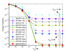
Figure 3: Outage probability performance comparison between ZPiORA, MEPPR and optimal QPA

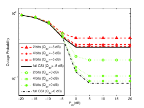
Figure 5: Effect of increasing feedback bits on outage performance of SU

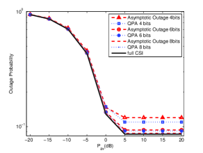
Figure 6: Comparison between asymptotic outage performance and QPA performance with $Q_{av}=0dB$

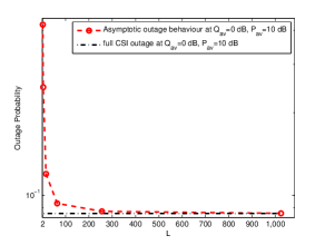
Figure 7: Asymptotic outage behaviour versus the number of quantization level $L$

In this section, we will examine the outage probability performance of the SU in a narrowband spectrum sharing system with the proposed power allocation strategies via numerical simulations. All the channels involved are assumed to be independent and undergo identical Rayleigh fading, i.e, channel power gain $g_{0}$ and $g_{1}$ are independent and identically exponentially distributed with unity mean. The required transmission rate is taken to be $r_{0}=0.25$ nats per channel use.
Fig. 3 displays the SU outage probability performance of the suboptimal algorithm ZPiORA versus $P_{av}$ with feedback bits $B=\{1,2\}$, under $Q_{av}=-5$ dB and $Q_{av}=0$ dB respectively, and compares these results with the corresponding outage performance of the suboptimal method MEPPR and the optimal QPA. As observed from Fig. 3, when $Q_{av}=-5$ dB, with $B$ fixed, the outage performances of ZPiORA and corresponding optimal QPA almost overlap with each other. When $Q_{av}=0$ dB and $P_{av}\leq-5$ dB, with the same number of feedback bits, the outage performances of these two methods are still indistinguishable; and with $P_{av}>-5$ dB, the outage performance gap between ZPiORA and corresponding optimal QPA is decreasing with increasing B. For example, with 1 bit feedback, at $P_{av}=10$ dB, the outage gap between ZPiORA and optimal QPA is $0.0347$, but with 2 bits of feedback, the outage performance of these two methods are very close to each other, which agrees with Lemma 2 that ZPiORA is a near-optimal algorithm for large number of feedback bits. Now we look at the performance comparison between ZPiORA and MEPPR. As illustrated in Fig. 3, when $P_{av}$ or ${Q_{av}}$ is small, with B bits feedback, the performance of ZPiORA is always better than MEPPR. This is attributed to the fact that when $P_{av}$ or ${Q_{av}}$ is small, it can be easily verified that $p_{L}$ is close to zero, but MEPPR always uses $p_{L}>0$. However, when both $P_{av}$ and $Q_{av}$ are large (e.g. $P_{av}\geq 0$ dB and $Q_{av}=0$ dB), for 1 bit feedback case, MEPPR outperforms ZPiORA and performs very close to the optimal QPA, whereas with a sufficiently large number of feedback bits (in fact, with more than just 2 bits of feedback), ZPiORA is a more accurate approximation due to Lemma 2. These results confirm the ZPiORA is a better option for a large number of feedback bits, not to mention that ZPiORA is much simpler to implement than MEPPR.
In addition, Fig. 4 compares the outage performance of ZPiORA with another suboptimal method (GLASFA) with $Q_{av}=-5$ dB. We can easily observe that with a fixed number of feedback bits (2 bits or 4 bits), ZPiORA always outperforms GLASFA. And ZPiORA is also substantially faster than GLASFA. For example, with fixed $\lambda$ and $\mu$ and 4 bits of feedback ($Q_{av}=-5$dB, $P_{av}=10$ dB), when implemented in MATLAB (version 7.11.0.584 (R2010b)) on a AMD Quad-Core processor (CPU P940 with a clock speed of $1.70$ GHz and a memory of 4 GB), it was seen that GLASFA (with 100,000 training samples, starting $k=20$ and increasing it by a factor of 1.5 at each step which finally converged at about $k=768.8672$) took approximately 299.442522 seconds (different initial guesses of the power codebook may result in different convergence time). In comparison, ZPiORA took only 0.006237 seconds to achieve comparable levels of accuracy. These results further confirm the efficiency of ZPiORA.
Fig. 5 illustrates the outage performance of SU with optimal QPA strategy versus $P_{av}$ with feedback bits $B=\{2,4,6\}$, under $Q_{av}=-5$ dB and $Q_{av}=0$ dB respectively, and studies the effect of increasing the number of feedback bits on the outage performance. For comparison, we also plot the corresponding SU outage performance with full CSI case. Since ZPiORA is an efficient suboptimal method for large number of feedback bits, we employ ZPiORA to obtain the outage performance instead of using optimal QPA for $B=6$ bits. First, it can be easily observed that all the outage curves decrease gradually as $P_{av}$ increases until $P_{av}$ reaches a certain threshold, when the outage probability attains a floor. This is due to the fact that in the high $P_{av}$ regime, the AIP constraint dominates. For a fixed number of feedback bits, the higher $Q_{av}$ is, the smaller the resultant outage probability is, since higher $Q_{av}$ means PU can tolerate more interference. Fig. 5 also illustrates that for fixed $Q_{av}$, introducing one extra bit of feedback substantially reduces the outage gap between QPA and the perfect CSI case. To be specific, for $Q_{av}=0$ dB and $P_{av}=10$ dB, with $2$ bits, $4$ bits and $6$ bits of feedback, the outage gaps with the full CSI case are approximately $0.1083$, $0.0249$ and $0.006979$ respectively. And for any $Q_{av}$, only 6 bits of feedback seem to result in an SU outage performance very close to that with full CSI case.
Figure 6 compares the asymptotic outage performance derived in Theorem 1 and the optimal QPA performance $B=\{4,6,8\}$ under $Q_{av}=0$ dB. It is clearly observed that increasing number of feedback bits substantially shrinks the outage performance gap between the asymptotic outage approximation and the corresponding optimal QPA performance. For instance, with 4, 6, 8 bits of feedback at $P_{av}=10$ dB, the outage gap between the asymptotic outage approximation and the corresponding optimal QPA are around $0.0325$, $0.00618$, $0.000168$ respectively. These results confirm that the derived asymptotic outage expressions in Theorem 1 are highly accurate for $B\geq 8$ bits of feedback. In addition, Figure 7 depicts the asymptotic outage probability behavior of SU versus the number of quantization level $L$ at $Q_{av}=0$ dB, $P_{av}=10$ dB, and compares the result with the corresponding full CSI performance. It can be seen from Figure 7 that the outage decreases as the number of quantization level $L$ increases, however, as $L$ increases beyond a certain number ($L\geq 2^{8}$, i.e, $B\geq 8$ bits), the outage probability curve starts to saturate and approaches the full CSI performance. This further confirms that only a small number of feedback bits is enough to obtain an outage performance close to the perfect CSI-based performance.

VI Conclusions and extensions

In this paper, we designed optimal power allocation algorithms for secondary outage probability minimization with quantized CSI information for a narrowband spectrum sharing cognitive radio framework under an ATP constraint at SU-TX and an AIP constraint at PU-RX. We prove that the optimal channel partition structure has a “stepwise” pattern based on which an efficient optimal power codebook design algorithm is provided. In the case of a large number of feedback bits, we derive a novel low-complexity suboptimal algorithm ZPiORA which is seen to outperform alternative suboptimal algorithms based on approximations used in the existing literature. We also derive explicit expressions for asymptotic behavior of the SU outage probability for a large number of feedback bits. Although the presented optimal power codebook design methods result in locally optimal solutions (due to the non-convexity of the quantized power allocation problem), numerical results illustrate that only 6 bits of feedback result in SU outage performance very close to that obtained with full CSI at the SU transmitter. Future work will involve extending the results to more complex wideband spectrum sharing scenario along with consideration of other types of interference constraints at the PU receiver.

-A Proof of Lemma 1:

We use an analysis method similar to [23] to prove our problem’s optimal quantizer structure. Let ${\cal{P}}=\{p_{1},\dots,p_{L}\}$, where $p_{1}>\dots>p_{L}\geq 0$, and the corresponding channel partitioning ${\cal{R}}=\{{\cal{R}}_{1},\dots,{\cal{R}}_{L}\}$ denote the optimal solution to the optimization problem (2), and $p(g_{0},g_{1})=p_{j},~{}~{}\text{if}~{}~{}(g_{0},g_{1})\in{\cal{R}}_{j}$.
Let ${\cal{R}}^{*}_{j}=\{(g_{0},g_{1}):v_{j}\leq g_{1}<v_{j+1},0\leq g_{0}<s_{j}\},~{}j=1,\dots,L-1$ and ${\cal{R}}^{*}_{L}={\cal{R}}^{*}_{L1}\cup{\cal{R}}^{*}_{L2}=\{(g_{0},g_{1}):v_{j}\leq g_{1}<v_{j+1},~{}g_{0}\geq s_{j},\forall j=0,1,\dots,L-1\}\cup\{(g_{0},g_{1}):g_{1}\geq v_{L},g_{0}\geq 0\}$, where $s_{0}=0$ and $v_{0}=0$. We assume that the set ${\cal{R}}^{*}_{j}\setminus{\cal{R}}_{j}$ is a non-empty set, where $\setminus$ is the set subtraction operation (i.e, if $(g_{0},g_{1})\in{\cal{R}}^{*}_{j}\setminus{\cal{R}}_{j}$, then $(g_{0},g_{1})\in{\cal{R}}^{*}_{j}$ but $(g_{0},g_{1})\notin{\cal{R}}_{j}$). Then, the set ${\cal{R}}^{*}_{j}\setminus{\cal{R}}_{j}$ can be partitioned into two subsets $S^{-}_{j}=({\cal{R}}^{*}_{j}\setminus{\cal{R}}_{j})\cap(\cup^{j-1}_{k=1}{\cal{R}}_{k})$ and $S^{+}_{j}=({\cal{R}}^{*}_{j}\setminus{\cal{R}}_{j})\cap(\cup^{L}_{k=j+1}{\cal{R}}_{k})$. In what follows, we denote the empty set by $\emptyset$.
(1): We will show that $S^{-}_{j}=\emptyset,~{}\forall j=1,\dots,L$.
(a): When $j=1$, it is obvious that $S^{-}_{1}=\emptyset$. When $1<j<L$, if $S^{-}_{j}\not=\emptyset$, then we can always reassign the set $S^{-}_{j}$ into region ${\cal{R}}_{j}$ without changing the overall outage probability. This is due to the fact that within the set $S^{-}_{j}\in{\cal{R}}^{*}_{j}$, we have $v_{j}\leq g_{1}<v_{j+1}$ resulting in $\frac{1}{2}\log(1+g_{1}p_{j})\geq r_{0}$, and the power level in $(\cup^{j-1}_{k=1}{\cal{R}}_{k})$ satisfies $p_{k}>p_{j}$. Thus $S^{-}_{j}$ is never in outage. However, the new assignment can achieve a lower Lagrange dual function (LDF) in (3), due to $g^{\prime}(\lambda,\mu)-g(\lambda,\mu)=E[(\lambda+\mu g_{0})(p_{j}-p_{k})|S^{-}_{j}]Pr(S^{-}_{j})<0$, where $g^{\prime}(\lambda,\mu)$ denotes the LDF with the new assignment, which contradicts the optimality of the solution ${\cal{P}},{\cal{R}}$.
(b) When $j=L$, if $S^{-}_{L}\not=\emptyset$, we can again reassign the set $S^{-}_{L}$ into region ${\cal{R}}_{L}$. 1) If some part of $S^{-}_{L}$ is in the set $\{(g_{0},g_{1}):0\leq g_{1}<v_{1},~{}g_{0}\geq 0\}$ of ${\cal{R}}^{*}_{L1}$, we have $\frac{1}{2}\log(1+g_{1}p_{1})<r_{0}$, which implies that this part of $S^{-}_{L}$ is always in outage. Therefore, this reassignment for this part of $S^{-}_{L}$ will not change the outage probability but will decrease the LDF due to the power level $p_{L}$ in ${\cal{R}}_{L}$ is the lowest. 2) For any $j$ ($j=1,\dots,L-1$), if some part of $S^{-}_{L}$ (denoted by “$S^{-}_{Lp}$”) exists in the set $\{(g_{0},g_{1}):v_{j}\leq g_{1}<v_{j+1},~{}g_{0}\geq s_{j}\}$ of ${\cal{R}}^{*}_{L1}$, we have $\frac{1}{2}\log(1+g_{1}p_{j})\geq r_{0}$, $\frac{1}{2}\log(1+g_{1}p_{j+1})<r_{0}$ and $(\lambda+\mu g_{0})(p_{j}-p_{L})\geq 1$. And given $S^{-}_{Lp}\subset(\cup^{L-1}_{k=1}{\cal{R}}_{k})$, let the power level for $S^{-}_{Lp}$ be $p_{k}$ (where $k$ could be any value from $\{1,\dots,L-1\}$). Reassigning this part of set $S^{-}_{L}$ into region ${\cal{R}}_{L}$ will reduce the value of the LDF, since if $k\leq j$ (implying $p_{k}\geq p_{j}$), $g^{\prime}(\lambda,\mu)-g(\lambda,\mu)=E[1+p_{L}(\lambda+\mu g_{0})-p_{k}(\lambda+\mu g_{0})|S^{-}_{Lp}]Pr(S^{-}_{Lp})<0$ and if $k>j$ (implying $p_{k}<p_{j}$), $g^{\prime}(\lambda,\mu)-g(\lambda,\mu)=E[1+p_{L}(\lambda+\mu g_{0})-1-p_{k}(\lambda+\mu g_{0})|S^{-}_{Lp}]Pr(S^{-}_{Lp})<0$. 3) If some part of $S^{-}_{L}$ belongs to the set ${\cal{R}}^{*}_{L2}$, similar to (a), we can show that the new partition for this part of $S^{-}_{L}$ does not change the overall outage probability and meanwhile reduces the value of the LDF. These all contradict optimality.
(2): We will now show that the set $S^{+}_{j}=\emptyset,~{}j=1,\dots,L$. When $j=L$, it’s straightforward that $S^{+}_{L}=\emptyset$. When $j<L$, we assume that $S^{+}_{j}\not=\emptyset$. Within the set $S^{+}_{j}\in{\cal{R}}^{*}_{j}$, we have $v_{j}\leq g_{1}<v_{j+1}$, implying $\frac{1}{2}\log(1+g_{1}p_{j+1})<r_{0}$, or in other words, $S^{+}_{j}\in(\cup^{L}_{k=j+1}{\cal{R}}_{k})$ is in outage. We can reallocate the set $S^{+}_{j}$ into region ${\cal{R}}_{j}$. This reassignment not only lowers the outage probability ($S^{+}_{j}$ with $p_{j}$ will not be in outage) but also lowers the value of the LDF, given by $g^{\prime}(\lambda,\mu)-g(\lambda,\mu)=E[(\lambda+\mu g_{0})(p_{j}-p_{k})-1|S^{+}_{j}]Pr(S^{+}_{j})\leq E[(\lambda+\mu g_{0})(p_{j}-p_{L})-1|S^{+}_{j}]Pr(S^{+}_{j})<0$, due to $g_{0}<s_{j}=\frac{1}{\mu(p_{j}-p_{L})}-\frac{\lambda}{\mu}$. This also contradicts optimality.
Therefore, we have ${\cal{R}}^{*}_{j}\setminus{\cal{R}}_{j}=\emptyset,~{}\forall j=1,\dots,L$, i.e, ${\cal{R}}^{*}_{j}\subseteq{\cal{R}}_{j},~{}\forall j=1,\dots,L$. Since $\cup^{L}_{j=1}{\cal{R}}^{*}_{j}=\text{the whole space of}~{}(g_{0},g_{1})=\cup^{L}_{j=1}{\cal{R}}_{j}$, and ${\cal{R}}^{*}_{j}\subseteq{\cal{R}}_{j},~{}\forall j$, we can obtain that ${\cal{R}}^{*}_{j}={\cal{R}}_{j},~{}\forall j=1,\dots,L.$

-B Proof of Lemma 2:

We assume that $\lim_{L\rightarrow\infty}p_{L}\not=0$. Let $\delta=\lim_{L\rightarrow\infty}p_{L}>0$. From the KKT condition (8), we have

$$e^{-v_{L}}\frac{c}{p^{2}_{L}}(p_{L-1}-p_{L})(\lambda+\mu(1-e^{-s_{L-1}})) =(\lambda+\mu)(P^{L}_{out}+e^{-v_{L}})+\mu\sum^{L-1}_{j=1}(e^{-v_{j}}-e^{-v_{j+1}})e^{-s_{j}}s_{j}$$

$$\geq(\lambda+\mu)(P^{L}_{out}+e^{-v_{L}})$$ (14)

Let $P^{f}_{out}$ denote the outage probability with full CSI at SU-TX, then we have $P^{L}_{out}\geq P^{f}_{out}$ and $\lim_{L\rightarrow\infty}P^{L}_{out}=P^{f}_{out}$. Taking the limit $L\rightarrow\infty$ on both sides of (14), we have

$$\lim_{L\rightarrow\infty}e^{-v_{L}}\frac{c}{p^{2}_{L}}(p_{L-1}-p_{L})(\lambda+\mu(1-e^{-s_{L-1}}))\geq(\lambda+\mu)(P^{f}_{out}+e^{-\frac{c}{\delta}})\not=0$$ (15)

Given $p_{1}>\dots>p_{L}>0$, it is clear that the sequence $\{p_{j}\},\;j=1,2,\ldots,L$ is a monotonically decreasing sequence bounded below, therefore it must converge to its greatest-lower bound $\delta$, as $L\rightarrow\infty$. Therefore, it can be easily shown that for an arbitrarily small $\epsilon>0$, we can always find a sufficiently large $L$ such that $p_{L-1}-p_{L}<\epsilon$. Thus, as $L\rightarrow\infty$, $(p_{L-1}-p_{L})\rightarrow 0$, which implies when $\mu>0$, $s_{L-1}=\frac{1}{\mu(p_{L-1}-p_{L})}-\frac{\lambda}{\mu}\rightarrow\infty$. This implies that

$$\lim_{L\rightarrow\infty}e^{-v_{L}}\frac{c}{p^{2}_{L}}(p_{L-1}-p_{L})(\lambda+\mu(1-e^{-s_{L-1}}))=e^{-\frac{c}{\delta}}\frac{c}{\delta^{2}}(\lambda+\mu)\lim_{L\rightarrow\infty}(p_{L-1}-p_{L})=0.$$ (16)

which is in contradiction with (15). Thus, we must have $\lim_{L\rightarrow\infty}p_{L}=0$.

-C Proof of Lemma 3:

As $L\rightarrow\infty$, from Lemma 2, we have $p_{L}\rightarrow 0$. Applying it to Problem (5), we have the KKT conditions as (10).
1) $\mu>0$: From $s^{\prime}_{j}=\frac{1}{\mu p_{j}}-\frac{\lambda}{\mu}$, we have $p_{j}=\frac{1}{\lambda+\mu s^{\prime}_{j}}$, and we also have $p_{0}=\frac{1}{\lambda+\mu s^{\prime}_{0}}$. Applying it to (10), the right hand side (RHS) of equation (10) becomes,

$$RHS =e^{-v_{j}}\frac{c}{p^{2}_{j}}[\frac{\lambda+\mu(1-e^{-s^{\prime}_{j-1}})}{\lambda+\mu s^{\prime}_{j-1}}-\frac{\lambda+\mu(1-e^{-s^{\prime}_{j}})}{\lambda+\mu s^{\prime}_{j}}]$$

$$=e^{-v_{j}}\frac{c(s^{\prime}_{j-1}-s^{\prime}_{j})}{p^{2}_{j}}\frac{\frac{\lambda+\mu(1-e^{-s^{\prime}_{j-1}})}{\lambda+\mu s^{\prime}_{j-1}}-\frac{\lambda+\mu(1-e^{-s^{\prime}_{j}})}{\lambda+\mu s^{\prime}_{j}}}{s^{\prime}_{j-1}-s^{\prime}_{j}}$$ (17)

From the mean value theorem (MVT), we have

$$\frac{\frac{\lambda+\mu(1-e^{-s^{\prime}_{j-1}})}{\lambda+\mu s^{\prime}_{j-1}}-\frac{\lambda+\mu(1-e^{-s^{\prime}_{j}})}{\lambda+\mu s^{\prime}_{j}}}{s^{\prime}_{j-1}-s^{\prime}_{j}}=\frac{-\mu}{(\lambda+\mu s^{\prime})^{2}}[\lambda(1-e^{-s^{\prime}})+\mu(1-e^{-s^{\prime}}(1+s^{\prime}))]$$ (18)

where $s^{\prime}\in[s^{\prime}_{j-1},s^{\prime}_{j})$. As the number of feedback bits $B=\log_{2}L\rightarrow\infty$, the length of quantization interval on $g_{0}$ axis $[s^{\prime}_{j-1},s^{\prime}_{j}),j=1,\dots,L-1$ approaches zero [20]. Hence (18) becomes,

$$\frac{\frac{\lambda+\mu(1-e^{-s^{\prime}_{j-1}})}{\lambda+\mu s^{\prime}_{j-1}}-\frac{\lambda+\mu(1-e^{-s^{\prime}_{j}})}{\lambda+\mu s^{\prime}_{j}}}{s^{\prime}_{j-1}-s^{\prime}_{j}}\approx\frac{-\mu}{(\lambda+\mu s^{\prime}_{j})^{2}}[\lambda(1-e^{-s^{\prime}_{j}})+\mu(1-e^{-s^{\prime}_{j}}(1+s^{\prime}_{j}))]$$ (19)

Applying (19) to (17), we have $RHS\approx e^{-v_{j}}c\mu(s^{\prime}_{j}-s^{\prime}_{j-1})[\lambda(1-e^{-s^{\prime}_{j}})+\mu(1-e^{-s^{\prime}_{j}}(1+s^{\prime}_{j}))]$. Similarly, as $L\rightarrow\infty$, we also have the length of quantization interval on the $g_{1}$ axis $[v_{j},v_{j+1}),j=1,\dots,L-2$ approaches zero, thus from MVT, $e^{-v_{j}}-e^{-v_{j+1}}\approx e^{-v_{j}}(v_{j+1}-v_{j})$. Thus the left hand side (LHS) of equation (10) can be approximated as, $LHS\approx e^{-v_{j}}(v_{j+1}-v_{j})[\lambda(1-e^{-s^{\prime}_{j}})+\mu(1-e^{-s^{\prime}_{j}}(1+s^{\prime}_{j}))$. Hence, we have $\forall j=1,\dots,L-2,$ $v_{j+1}-v_{j}\approx c\mu(s^{\prime}_{j}-s^{\prime}_{j-1})$, from which we get $s^{\prime}_{j+1}-s^{\prime}_{j}\approx s^{\prime}_{j}-s^{\prime}_{j-1},\forall j=1,\dots,L-2$, namely, $s^{\prime}_{L-1}-s^{\prime}_{L-2}\approx\dots\approx s^{\prime}_{1}-s^{\prime}_{0}$, since $v_{j}=c\lambda+c\mu s^{\prime}_{j}$.

2) $\mu=0$: In this case, we have $s^{\prime}_{j}=\infty,j=1,\dots,L-1$. Thus (10) becomes $e^{-v_{j}}-e^{-v_{j+1}}=e^{-v_{j}}\frac{c}{p^{2}_{j}}(p_{j-1}-p_{j})$, where $j=1,\dots,L-1$ and $p_{0}=\frac{1}{\lambda}$, which can be rewritten as $\frac{1}{v_{j}}(e^{-v_{j}}-e^{-v_{j+1}})=\frac{1}{v_{j-1}}e^{-v_{j}}(v_{j}-v_{j-1})$, where $v_{0}=\frac{c}{p_{0}}=c\lambda$. Applying MVT into as before, we have $\frac{1}{v_{j}}e^{-v_{j}}(v_{j+1}-v_{j})\approx\frac{1}{v_{j-1}}e^{-v_{j}}(v_{j}-v_{j-1}),\forall j=1,\dots,L-2$, which yields $\frac{v_{j+1}}{v_{j}}\approx\frac{v_{j}}{v_{j-1}},\forall j=1,\dots,L-2$, namely, $\frac{v_{L-1}}{v_{L-2}}\approx\dots\approx\frac{v_{1}}{v_{0}}$.

This completes the proof for Lemma 3.

-D Proof of Lemma 4:

As $L\rightarrow\infty$, from Lemma 2, we have $p_{L}\rightarrow 0$. Adding the two equations of (9) together and applying $p_{L}\rightarrow 0$, we have

$$\sum^{L-1}_{j=1}p_{j}(e^{-v_{j}}-e^{-v_{j+1}})[\lambda(1-e^{-s^{\prime}_{j}})+\mu(1-e^{-s^{\prime}_{j}}(1+s^{\prime}_{j}))]=\lambda P_{av}+\mu Q_{av}$$ (20)

The KKT conditions (10) can be rewritten as

$$p_{j}(e^{-v_{j}}-e^{-v_{j+1}})[\lambda(1-e^{-s^{\prime}_{j}})+\mu(1-e^{-s^{\prime}_{j}}(1+s^{\prime}_{j}))]=p_{j-1}e^{-v_{j}}(v_{j}-v_{j-1})\frac{[\hat{f}^{\prime}(p_{j-1})-\hat{f}^{\prime}(p_{j})]}{p_{j-1}-p_{j}}$$ (21)

where $\hat{f}^{\prime}(p_{j})=p_{j}(\lambda+\mu(1-e^{-s^{\prime}_{j}}))$. As mentioned before, when $L\rightarrow\infty$, we have the length of quantization interval on the $g_{1}$ axis $[v_{j-1},v_{j}),j=2,\dots,L-1$ approaching zero. Hence we also have the length of the interval $[p_{j-1},p_{j}),j=2,\dots,L-1$ approaching zero, since $v_{j}=\frac{c}{p_{j}}$. Thus from MVT, we have

$$e^{-v_{j-1}}-e^{-v_{j}} \approx e^{-v_{j}}(v_{j}-v_{j-1})$$

$$\frac{\hat{f}^{\prime}(p_{j-1})-\hat{f}^{\prime}(p_{j})}{p_{j-1}-p_{j}} \approx\lambda(1-e^{-s^{\prime}_{j-1}})+\mu(1-e^{-s^{\prime}_{j-1}}(1+s^{\prime}_{j-1}))$$ (22)

Applying (22) into (21), we can obtain, $\forall j=2,\dots,L-1$

$$p_{j}(e^{-v_{j}}-e^{-v_{j+1}})[\lambda(1-e^{-s^{\prime}_{j}})+\mu(1-e^{-s^{\prime}_{j}}(1+s^{\prime}_{j}))]\approx$$

$$p_{j-1}(e^{-v_{j-1}}-e^{-v_{j}})[\lambda(1-e^{-s^{\prime}_{j-1}})+\mu(1-e^{-s^{\prime}_{j-1}}(1+s^{\prime}_{j-1}))]$$ (23)

Then applying the result of (23) into (20), we can have $j=1,\dots,L-1$

$$p_{j}(e^{-v_{j}}-e^{-v_{j+1}})[\lambda(1-e^{-s^{\prime}_{j}})+\mu(1-e^{-s^{\prime}_{j}}(1+s^{\prime}_{j}))]\approx\frac{\lambda P_{av}+\mu Q_{av}}{L-1}$$ (24)

which gives,

$$\sum^{L-1}_{j=1}(e^{-v_{j}}-e^{-v_{j+1}})[\lambda(1-e^{-s^{\prime}_{j}})+\mu(1-e^{-s^{\prime}_{j}}(1+s^{\prime}_{j}))]\approx\frac{\lambda P_{av}+\mu Q_{av}}{L-1}\sum^{L-1}_{j=1}\frac{1}{p_{j}}.$$ (25)

This completes the proof for Lemma 4.

-E Proof of Theorem 1:

1) $\mu>0$: From Lemma 3, we can easily obtain, $s^{\prime}_{j}\approx js^{\prime}_{1},\;\frac{1}{p_{j}}=\lambda+\mu s^{\prime}_{j}\approx\lambda+j\mu s^{\prime}_{1}$, and ${v_{j}}=\frac{c}{p_{j}}\approx c\lambda+jc\mu s^{\prime}_{1},\forall j=1,\dots,L-1$, Let $z=\sum^{L-1}_{j=1}(e^{-v_{j}}-e^{-v_{j+1}})[\lambda(1-e^{-s^{\prime}_{j}})+\mu(1-e^{-s^{\prime}_{j}}(1+s^{\prime}_{j}))]$, which implies that $0<z<\lambda+\mu$. Then from Lemma 4, we have $\frac{1}{L-1}\sum^{L-1}_{j=1}\frac{1}{p_{j}}\approx z^{\prime}$, where $z^{\prime}=\frac{z}{\lambda P_{av}+\mu Q_{av}}$ and $0<z^{\prime}<\frac{\lambda+\mu}{\lambda P_{av}+\mu Q_{av}}$. Using the above results, we get $s^{\prime}_{1}\approx\frac{2(z^{\prime}-\lambda)}{\mu L}=\frac{d}{L}$, where $d=\frac{2(z^{\prime}-\lambda)}{\mu}$. Let $a=c\mu d=2(z^{\prime}-\lambda)c$, then $s^{\prime}_{1}\approx\frac{a}{c\mu L}$. Since $0<z^{\prime}<\frac{\lambda+\mu}{\lambda P_{av}+\mu Q_{av}}$, we have $\lim_{L\rightarrow\infty}\frac{a}{L}=0$. From the definition of $z$ above, we have

$$z =(\lambda+\mu)e^{-v_{1}}-\sum^{L-1}_{j=1}(e^{-v_{j}}-e^{-v_{j+1}})[(\lambda+\mu)e^{-s^{\prime}_{j}}+\mu e^{-s^{\prime}_{j}}s^{\prime}_{j}]$$

$$\approx e^{-c\lambda}[(\lambda+\mu)e^{-\frac{a}{L}}-(1-e^{-\frac{a}{L}})(\lambda+\mu)\sum^{L-1}_{j=1}e^{-j(\frac{a}{L}+s^{\prime}_{1})}-(1-e^{-\frac{a}{L}})\mu s^{\prime}_{1}\sum^{L-1}_{j=1}je^{-j(\frac{a}{L}+s^{\prime}_{1})}]$$

$$\approx e^{-c\lambda}[(\lambda+\mu)e^{-\frac{a}{L}}-(1-e^{-\frac{a}{L}})(\lambda+\mu)\sum^{L-1}_{j=1}e^{-j\frac{b}{L}}-(1-e^{-\frac{a}{L}})\frac{a}{cL}\sum^{L-1}_{j=1}je^{-j\frac{b}{L}}]$$ (26)

where $b=a+Ls^{\prime}_{1}=a(1+\frac{1}{c\mu})$ and we also have $\lim_{L\rightarrow\infty}\frac{b}{L}=0$. Since $\sum^{L-1}_{j=1}e^{-j\frac{b}{L}}=\frac{1-e^{-b}}{1-e^{-\frac{b}{L}}}-1$, and $\sum^{L-1}_{j=1}je^{-j\frac{b}{L}}=-\frac{e^{(-\frac{b}{L}-b)}(Le^{\frac{b}{L}}-e^{b}-L+1)}{(1-e^{-\frac{b}{L}})^{2}}$, (26) becomes

$$z \approx e^{-c\lambda}[(\lambda+\mu)(1-(1-e^{-\frac{a}{L}})\frac{1-e^{-b}}{1-e^{-\frac{b}{L}}})-(1-e^{-\frac{a}{L}})\frac{a}{cL}\frac{e^{-\frac{b}{L}}(1-e^{-b})-Le^{-b}(1-e^{-\frac{b}{L}})}{(1-e^{-\frac{b}{L}})^{2}}]$$ (27)

Since $\lim_{L\rightarrow\infty}\frac{a}{L}=0$ and $\lim_{L\rightarrow\infty}\frac{b}{L}=0$, we have $1-e^{-\frac{a}{L}}\approx\frac{a}{L}$ and $1-e^{-\frac{b}{L}}\approx\frac{b}{L}$. And when $L\rightarrow\infty$, we approach the full CSI scenario, thus implying $\lambda\approx\lambda^{f},\mu\approx\mu^{f}$. Using these results in (27), we have

$$z \approx e^{-c\lambda_{f}^{*}}[(\lambda_{f}^{*}+\mu_{f}^{*})(1-\frac{a}{b}(1-e^{-b}))-\frac{a^{2}}{cb^{2}}((1-\frac{b}{L})(1-e^{-b})-be^{-b})]$$

$$\approx e^{-c\lambda_{f}^{*}}[(\lambda_{f}^{*}+\mu_{f}^{*})(1-\frac{a}{b}(1-e^{-b}))-\frac{a^{2}}{cb^{2}}(1-e^{-b}(1+b))]$$ (28)

Since $z=(\lambda P_{av}+\mu Q_{av})z^{\prime}=(\lambda P_{av}+\mu Q_{av})(\lambda+\frac{a}{2c})\approx(\lambda_{f}^{*}P_{av}+\mu_{f}^{*}Q_{av})(\lambda_{f}^{*}+\frac{a}{2c})$, we can obtain $a$ from the following approximation:

$$(\lambda_{f}^{*}P_{av}+\mu_{f}^{*}Q_{av})(\lambda_{f}^{*}+\frac{a}{2c})e^{c\lambda_{f}^{*}}$$

$$\approx[(\lambda_{f}^{*}+\mu_{f}^{*})(1-\frac{c\mu_{f}^{*}}{1+c\mu_{f}^{*}}(1-e^{-a(1+\frac{1}{c\mu_{f}^{*}})}))-\frac{c(\mu_{f}^{*})^{2}}{(1+c\mu_{f}^{*})^{2}}(1-e^{-a(1+\frac{1}{c\mu_{f}^{*}})}(1+a(1+\frac{1}{c\mu_{f}^{*}})))]$$ (29)

From (29), with given $P_{av}$ and $Q_{av}$, $a$ is a constant. Then when $L$ is large,

$$P^{L}_{out} \approx 1-e^{-v_{1}}+\sum^{L-1}_{j=1}(e^{-v_{j}}-e^{-v_{j+1}})e^{-s^{\prime}_{j}}\approx 1-e^{-c\lambda}[e^{-\frac{a}{L}}-(1-e^{-\frac{a}{L}})\sum^{L-1}_{j=1}e^{-j\frac{b}{L}}]$$

$$=1-e^{-c\lambda}[1-(1-e^{-\frac{a}{L}})\frac{1-e^{-b}}{1-e^{-\frac{b}{L}}}]\approx 1-e^{-c\lambda_{f}^{*}}[1-(1-e^{-\frac{a}{L}})\frac{1-e^{-a(1+\frac{1}{c\mu_{f}^{*}})}}{1-e^{-\frac{a(1+\frac{1}{c\mu_{f}^{*}})}{L}}}]$$ (30)

and $\lim_{L\rightarrow\infty}P^{L}_{out}=1-e^{-c\lambda_{f}^{*}}[1-\frac{1-e^{-a(1+\frac{1}{c\mu_{f}^{*}})}}{1+\frac{1}{c\mu_{f}^{*}}}]$.
2) $\mu=0$: Let $y=\frac{v_{1}}{v_{0}}=\frac{v_{1}}{c\lambda}>1$, then again, from Lemma 3, we can get for $j=1,\dots,L-1$, $v_{j}\approx c\lambda y^{j}$. From Lemma 4, we have $e^{-c\lambda y}\approx\frac{\lambda P_{av}}{L-1}\sum^{L-1}_{j=1}y^{j}=\frac{\lambda P_{av}}{L-1}\frac{y^{L}-y}{y-1}$. With $x=y-1$, we have, $e^{-c\lambda(1+x)}\approx{\lambda P_{av}}(1+x)\frac{(1+x)^{L-1}-1}{x(L-1)}$. Now, suppose $\lim_{L\rightarrow\infty}xL=\infty$. Since $(1+x)^{L-1}>1+(L-1)x+\frac{1}{2}(L-2)(L-1)x^{2}$, we have $\lim_{L\rightarrow\infty}\frac{(1+x)^{L-1}-1}{(L-1)x}>\lim_{L\rightarrow\infty}1+\frac{1}{2}(L-2)x=\infty$. Then taking the limit as $L\rightarrow\infty$, we have $\lim_{L\rightarrow\infty}e^{-c\lambda(1+x)}=\infty$, which contradicts $\lim_{L\rightarrow\infty}e^{-c\lambda(1+x)}<1$, thus we must have $\lim_{L\rightarrow\infty}xL=0\leq\beta<\infty$ (where $\beta$ is a constant), implying as $L\rightarrow\infty$, $x\rightarrow\frac{\beta}{L}$. Applying this result, we get $e^{-c\lambda(1+\frac{\beta}{L})}\approx{\lambda P_{av}}(1+\frac{\beta}{L})\frac{(1+\frac{\beta}{L})^{L-1}-1}{\frac{\beta}{L}(L-1)}$. After taking the limit as $L\rightarrow\infty$ on both sides of above equation, we have $e^{-c\lambda_{f}^{*}}\approx{\lambda_{f}^{*}P_{av}}\frac{e^{\beta}-1}{\beta}$, from which one can solve for $\beta$ approximately. Note that in the above approximation, we have used $\lim_{L\rightarrow\infty}(1+\frac{\beta}{L})^{L-1}=e^{\beta}$ and when $L$ is large, $\lambda\approx\lambda_{f}^{*}$. Therefore, when $L$ is large, $P^{L}_{out}=1-e^{-v_{1}}=1-e^{-c\lambda(1+x)}\approx 1-e^{-c\lambda_{f}^{*}(1+\frac{\beta}{L})}$, $\lim_{L\rightarrow\infty}P^{L}_{out}=1-e^{-c\lambda_{f}^{*}}$.

This completes the proof for Theorem 1.

Figure 4: Outage probability performance comparison between ZPiORA and other possible suboptimal algorithm : GLASFA

References

- [1]
- [2]
- [3] J.M. Peha, “Sharing Spectrum Through Spectrum Policy Reform and Cognitive Radio,” Proc. of the IEEE, vol. 97, no. 4, pp. 708-719, Apr. 2009.
- [4] J. Mitola III, “Cognitive radio for flexible mobile multimedia communications,” IEEE Int. Workshop on Mobile Multimedia Commun. (MoMuC) , San Diego, CA, USA, Nov. 1999, pp. 3-10.
- [5] A. Goldsmith, S.A. Jafar, I. Maric, and S. Srinivasa, “Breaking spectrum gridlock with cognitive radios: an information theoretic perspective,” Proceedings of the IEEE, vol. 97, no. 5, pp. 894-914, May 2009.
- [6] X. Kang, Y. Liang, A. Nallanathan, H.K. Garg and R. Zhang, “Optimal power allocation for fading channels in cognitive radio networks: Ergodic capacity and outage capacity,” IEEE Trans. Wireless Commun., vol. 8, no. 2, pp. 940-950, Feb. 2009.
- [7] A. Ghasemi and E. S. Sousa, “Fundamental limits of spectrum-sharing in fading environments,” IEEE Trans. Wireless Commun., vol. 6, no. 2, pp. 649-658, Feb. 2007.
- [8] H. A. Suraweera, J. Gao, P. J. Smith, M. Shafi and M. Faulkner “Channel capacity limits of cognitive radio in asymmetric fading environments ,” IEEE International Conference on Commun. (ICC 2008) , Beijing, China, May 2008, pp. 4048 - 4053 .
- [9] L. Musavian and S. Aissa, “Capacity and power allocation for spectrum-sharing communications in fading channels,” IEEE Trans. Wireless Commun., vol. 8, no. 1, pp. 148-156, Jan. 2009.
- [10] L. Musavian and S. Aissa, “Fundamental capacity limits of cognitive radio in fading environments with imperfect channel information,” IEEE Trans. Commun., vol. 57, no. 11, pp. 3472-3480, Nov. 2009.
- [11] H.A. Suraweera, P.J. Smith and M. Shafi, “Capacity Limits and Performance Analysis of Cognitive Radio With Imperfect Channel Knowledge,” IEEE Transactions on Vehicular Technology, vol. 59, no. 4, pp. 1811-1822, February 2010.
- [12] K. Huang and R. Zhang “Cooperative feedback for multi-antenna cognitive radio networks ,” IEEE Transactions on Signal Processing, vol. 59, no. 2, pp. 747-758, February 2011.
- [13] L. Zhang, Y-C. Liang, Y. Xin and H.V. Poor, “Robust Cognitive Beamforming with Partial Channel State Information,” IEEE Transactions on Wireless Communications, vol. 8, no. 8, pp. 4143-4153, August 2009.
- [14] A.G. Marques, X. Wang and G.B. Giannakis, “Dynamic Resource Management for Cognitive Radios Using Limited-Rate Feedback,” IEEE Transactions on Signal Processing, vol. 57, no. 9, pp. 3651-3666, September 2009.
- [15] Y. Y. He and S. Dey “Power allocation in spectrum sharing cognitive radio networks with quantized channel information,” IEEE Trans. Commun., vol. 59, no. 6, pp. 1644-1656, June 2011,
- [16] S. Huang, X. Liu and Z. Ding, “Decentralized Cognitive Radio Control Based on Inference from Primary Link Control Information,” IEEE Journal on Selected Areas in Communications, vol. 29, no. 2, Feb. 2011.
- [17] K. Eswaran, M. Gastpar and K. Ramachandran, “Cognitive Radio Through Primary Control Feedback,” IEEE Journal on Selected Areas in Communications, vol. 29, no. 2, Feb. 2011.
- [18] R. Zhang, “On peak versus average interference power constraints for protecting primary users in cognitive radio networks,” IEEE Trans. Wireless Commun., vol. 8, no. 4, pp. 2112-2120, April 2009.
- [19] J. C. Spall, “Implementation of the simultaneous perturbation algorithm for stochastic optimization,” IEEE Transactions on Aerospace and Electronic Systems, vol. 34, no. 3, pp. 817–823, Jul. 1998.
- [20] A. Khoshnevis and A. Sabharwal, “Performance of quantized power control in multiple antenna systems,” in Proc. IEEE International Conference on Communication(ICC’04), Paris, France, Jun. 2004, pp. 803–807.
- [21] B. Khoshnevis and Wei Yu,“Joint Power Control and Beamforming Codebook Design for MISO Channels with Limited Feedback,” IEEE Global Telecommunications Conference(GLOBECOM 2009), Honolulu, HI, USA, Dec. 2009, pp. 1 - 6.
- [22] P. A. Chou, T. Lookabaugh and R. M. Gray “Entropy-Constrained Vector Quantization,” in IEEE TRANSACTIONS ON ACOUSTICS, SPEECH, AND SIGNAL PROCESSING, vol. 31, no. 1, pp. 31–42, Jan. 1989.
- [23] M. A. Khojastepour, G. Yue, X. Wang and M. Madihian, “Optimal power control in MIMO systems with quantized feedback,” IEEE Transactions on Wireless Communications, vol. 7, no. 12, pp. 4859–4866, Dec. 2008.