Optimized differential energy loss estimation for tracker detectors

Abstract

The estimation of differential energy loss for charged particles in tracker detectors is studied. The robust truncated mean method can be generalized to the linear combination of the energy deposit measurements. The optimized weights in case of arithmetic and geometric means are obtained using a detailed simulation. The results show better particle separation power for both semiconductor and gaseous detectors.

1 Introduction

The identification of charged particles is crucial in several fields of particle and nuclear physics: particle spectra, correlations, selection of daughters of resonance decays and for reducing the background of rare physics processes [1, 2]. Tracker detectors, both semiconductor and gaseous, can be employed for particle identification, or yield extraction in the statistical sense, by proper use of energy deposit measurements along the trajectory of the particle. While for gaseous detectors a wide momentum range is available, in semiconductors there is practically no logarithmic rise of differential energy loss ($\mathrm{d}E/\mathrm{d}x$) at high momentum, thus only momenta below the the minimum ionization region are accessible. In this work two representative materials, silicon and neon are studied. Energy loss of charged particles inside matter is a complicated process. For detailed theoretical model and several comparisons to measured data see Refs. [3, 4].

While the energy lost and deposited differ, they will be used interchangeably in the discussion. It is also clear that the energy read out also varies due to noise and digitization effects.

This article is organized as follows: Sec. 2 describes the microscopical energy loss simulation used in this study. Sec. 3 introduces the basic method of truncated mean, while Sec. 4 deals at length with the optimization of weighted arithmetic and geometric means. Possible handling of different path lengths is discussed in Sec. 5. Results of the simulation and applications of the optimized weighted means are shown in Sec. 6. The work ends with conclusions and it is supplemented by four Appendices with interesting results, such as optimal weights in case of few (App. A) and many measurements (App. B); some theoretical insights (App. C); also on connection to maximum likelihood estimation (App. D).

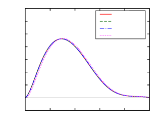
Figure 1: Comparison of differential energy loss distributions for 300 $\mu$m silicon (left) and 1 cm neon (right), at $\beta\gamma=3.17$. The probability density function (solid) is shown with theory motivated fits (dashed). Above a certain $\mathrm{d}E/\mathrm{d}x$ value, indicated by the vertical dash-dotted lines, a power function was used, while below that the product of a power and a Gaussian (silicon) or the product of a power and an exponential (neon) was taken. For details see App. C.

2 Simulation

When a charged particle traverses material it loses energy in several discrete steps, dominantly by resonance excitations ($\delta$-function) and Coulomb excitations (truncated power-law term). This latter is the reason for the long tail observed in energy deposit distributions.

The probability of an excitation, energy deposit, along the path of the incoming particle is a function of $\beta\gamma=p/m$ of the particle and depends on properties of the traversed material. The conditional probability density $p(\Delta|t)$, deposit $\Delta$ along a given path length $t$, can be built using the above mentioned elementary excitations combined with an exponential occurrence model. The details of the microscopical simulation can be found in Refs. [3], [4] and [5]. The result of these recursive convolutions is a smooth asymmetric density distribution with long tails (see Fig. 1, solid lines). In order to model detector and readout noise, Gaussian random values with standard deviation of 2 keV (0.01 keV) were added to each hit for silicon (neon). For further studies on noise dependence see Sec. 6.1.

3 Truncated mean

There are several possibilities for the estimation of the differential energy loss of a charged particle. An approach using some theoretical model of energy loss would enable to use advanced methods such as maximum likelihood estimation. However, especially at startup, particle detectors are not expected to be understood to the degree that would enable the use of such estimator. The results would be quite sensitive to the choice of the model, precision of detector gain calibration, the level of noise and several backgrounds.

One of the robust and simple estimators is the so called truncated mean that is traditionally used in gas filled detector chambers [6, 7]. It reduces the influence of high energy deposits in the tail of the energy deposit distribution. For this aim a given fraction of the upper 30-60% (and sometimes the lower 0-10%) measurements are discarded and only the remaining measurements are averaged with equal weights. Recent studies show that five or even four layers of silicon allow to reach 10% resolution, using the truncated mean method [2].

Let $\Delta_{i}$ denote the deposit and $t_{i}$ denote the path length in the active material of the detector, in case of the $i$th measurement of the particle trajectory. The differential energy loss is $y_{i}\equiv\Delta_{i}/t_{i}$. The numbering of the measurements is such that they are ordered: $y_{i}\leq y_{i+1}$, in case of $n$ space points ($i=1,2,\dots,n$). The estimator is simply

$$y=\frac{\sum_{i=1}^{n}w_{i}y_{i}}{\sum_{i=1}^{n}w_{i}}.$$

E.g. if only the lower half of the hits are used, (0%,50%) truncation, the corresponding weights $$w_{i}$$ are

$$w_{i}=\begin{cases}0&\text{if $2i>n+1$}\\ 1/2&\text{if $2i=n+1$}\\ 1&\text{if $2i<n+1$}.\end{cases}$$

In the rest of this paper by simple truncated mean we will mean this (0%,50%) truncation.

Figure 2: Correlation matrix of hits $(i,j)$ for 300 $\mu$m silicon (left) and 1 cm neon (right), at $\beta\gamma=3.17$, in case of 20 hits on track.

4 Weighted means

It is possible to generalize this estimator, and optimize the weights, by looking at some measures of its distribution. The generalization can be twofold. Instead of a simple truncated mean, the more general weighted mean, linear combination, can be examined where the constant weights are allowed to take on different values, not just 0, 1/2 or 1. In addition it is possible that the performance of the weighted mean is more beneficial when averaging a monotonic function of the measurements $x_{i}=R(y_{i})$ than just taking the $y_{i}$ values themselves. It is clear that the transformed values are also ordered: $x_{i}\leq x_{i+1}$. Let us look at the linear combination of $n$ measurements

$$y =R^{-1}\left(\sum_{i=1}^{n}w_{i}R(y_{i})\right), R(y)\equiv x =\sum_{i=1}^{n}w_{i}x_{i}$$ (1)

where $\sum_{i=1}^{n}w_{i}=1$. In the following two cases will be examined further. If $R$ is identity we get back the weighted arithmetic mean, the use of $R(y)=\log y$ gives the weighted geometric mean. While the former choice is historical and most simple, the geometric mean has its root in the behavior of energy loss distribution since that can be approximated by log-normal distribution. In that sense $\log(y)$ seems to have a more symmetric distribution than the long tailed $y$.

In fact an optimization of the transformation function $R$ could complete the study, but that task appears to be highly non-trivial. Both arithmetic and geometric means are special cases among power functions, $R(y)=y^{p}$, with $p=1$ and $p\rightarrow 0$, respectively:

$$y_{\text{arith}} =\sum w_{i}y_{i}, y_{\text{geom}} =\exp\left(\sum w_{i}\ln y_{i}\right).$$

Note that extreme cases $p=-\infty$ (minimum) and $p=\infty$ (maximum) are also included in the weighted arithmetic mean.

4.1 Goal of the optimization

In order to facilitate clean particle identification and extraction of particle yields, the distribution of the estimator should be narrow and should be sensitive to changes in the average energy loss. If the momentum of the particle or its mass is altered the distribution of deposited energy will change accordingly. A small change can be modelled by multiplying each energy deposit along the trajectory with a factor $1+\alpha$, where $\alpha$ is small. If the distribution of the estimator is close to Gaussian (mean $m$, standard deviation $\sigma$), its mean will shift. The separation power between the original and altered distributions, in units of standard deviation, will be

$$\frac{1}{\sigma}\frac{\partial m}{\partial\alpha}.$$

In case of the arithmetic mean, the estimator is linear, $\partial m/\partial\alpha=m$, thus the relative resolution $\sigma/m$ has to be minimized (see Sec. 4.2). For the geometric mean the multiplication corresponds to a shift $\alpha$, hence the the absolute resolution $\sigma$ is to be minimized (see Sec. 4.3).

The mean of the $i$th ordered measurement and the covariance of the $i$th and $j$th measurements play a central role in the optimization. They are determined as

$$m_{i} =\langle x_{i}\rangle, V_{ij} =\langle x_{i}x_{j}\rangle-\langle x_{i}\rangle\langle x_{j}\rangle.$$

Both $m_{i}$ and $V_{ij}$ can be estimated using detailed physics simulation described in Sec. 2. The correlation matrix for silicon and neon is shown in Fig. 2, for a given thickness and $\beta\gamma$ choice, in case of 20 hits on track. Higher deposits are strongly correlated, thus they contain less information and should get less weight than other hits. The mean and variance of the estimator $\sum_{i=1}^{n}w_{i}x_{i}$ (Eq. (1)) are

$$m =\sum_{i=1}^{n}m_{i}w_{i}, \sigma^{2} =\sum_{i,j=1}^{n}w_{i}V_{ij}w_{j}.$$ (2)

With help of optimized weights not only the differential energy loss, but also its variance can be estimated, a definite advantage over the simple truncated or other plain averages. The weights are of practical use if, for a wide range of number of hits on track, they appear independent of or insensitive to $\beta\gamma$ values and material thickness. In the following it is shown that this is indeed the case.

4.2 Weighted arithmetic mean

The task is to minimize the relative resolution

$$\frac{\sigma}{m}=\frac{\sqrt{{\bf w}^{T}V{\bf w}}}{{\bf m}{\bf w}}$$

by varying the weights ${\bf w}$. (Note that here we switched to vector and matrix forms.) The square of this quantity is

$$q({\bf w})=\frac{{\bf w}^{T}V{\bf w}}{({\bf w}^{T}{\bf m})({\bf m}^{T}{\bf w})}=\frac{{\bf w}^{T}V{\bf w}}{{\bf w}^{T}M{\bf w}}.$$

The term on the right side is a generalized Rayleigh quotient, $M={\bf m}\otimes{\bf m}^{T}$ is a dyadic matrix. For the first variation $\delta q$

$$\delta q=\frac{\delta[{\bf w}^{T}(V-qM){\bf w}]}{{\bf w}^{T}M{\bf w}}$$

A vector $${\bf w} q \delta q=0 V{\bf w}=qM{\bf w}$$ that minimizes must give and thus satisfy , which can be rearranged to get

$${\bf w}=q(V^{-1}{\bf m})({\bf m}^{T}{\bf w}).$$

Here the vectors ${\bf w}$ and $V^{-1}{\bf m}$ should be parallel. If sum of the weights has to be one, the optimal weights are

$${\bf w}=\frac{V^{-1}{\bf m}}{{\bf 1}^{T}V^{-1}{\bf m}}$$ (3)

where ${\bf 1}$ is a column vector of ones. It follows that the value of the relative resolution at the minimum is

$$\min\left(\frac{\sigma}{m}\right)=\sqrt{q}=\frac{1}{\sqrt{{\bf m}^{T}V^{-1}{\bf m}}}.$$

The sensitivity on the weights could be obtained from the Hessian

$$H=2\frac{V-qM}{({\bf w}^{T}{\bf m})({\bf m}^{T}{\bf w})}.$$

Since at minimum $H{\bf w}={\bf 0}$, according to Cramer’s rule $\operatorname{det}H=0$, so $H$ is singular. The sensitivity on weights, corresponding to 1% increase of the relative resolution, can be demonstrated as

$$\Delta w_{i}=\sqrt{10^{-2}\cdot 2q/H_{ii}}.$$ (4)

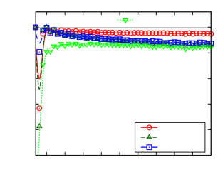
Figure 3: From top to bottom: normalization factors for 300 $\mu$m silicon and 1 cm neon, at various $\beta\gamma$ values; normalization factors in case of $\beta\gamma=3.17$ for silicon and neon, at various thicknesses. Lines are drawn to guide the eye.

4.3 Weighted geometric mean

The task is to minimize the variance $\sigma^{2}$, with the constraint $\sum_{i}w_{i}=1$. Thus, the expression to minimize is

$$q({\bf w})={\bf w}^{T}V{\bf w}+\lambda\left({\bf 1}^{T}{\bf w}-1\right).$$

Figure 4: Comparison of differential energy loss distributions for 300 $\mu$ silicon (left) and 1 cm neon (right), at $\beta\gamma=3.17$. The probability density function (solid) is shown with estimators obtained using the simple truncated mean (dashed) and the weighted arithmetic mean after optimization (dash-dotted), in case of 6 hits on track. The horizontal bar indicates the magnitude of noise (2 keV for silicon, 0.01 keV for neon), multiplied by a factor 10.

where $\lambda$ is a Lagrange multiplier. At the minimum there is linear system of equations to solve

$$2V{\bf w}+\lambda{\bf 1} ={\bf 0}, {\bf 1}^{T}{\bf w}-1 =0$$

or in matrix form

$$H\begin{pmatrix}{\bf w}\\ \lambda\end{pmatrix} =\begin{pmatrix}{\bf 0}\\ 1\end{pmatrix}, H =\begin{pmatrix}2V&{\bf 1}\\ {\bf 1}^{T}&0\end{pmatrix}$$

where $H$ is also the Hessian of $q$. The block matrix $H$ can be inverted

$$H^{-1}=\frac{1}{{\bf 1}^{T}V^{-1}{\bf 1}}\begin{pmatrix}-V^{-1}-V^{-1}{\bf 1}{\bf 1}^{T}V^{-1}&V^{-1}{\bf 1}\\ {\bf 1}^{T}V^{-1}&-2\end{pmatrix}$$

and the equations are solved. The optimal weights are

$${\bf w}=\frac{V^{-1}{\bf 1}}{{\bf 1}^{T}V^{-1}{\bf 1}}$$ (5)

while the multiplier is $\lambda=-2/({\bf 1}^{T}V^{-1}{\bf 1})$. A comparison of Eq. (3) and Eq. (5) shows that both expressions have a similar structure. It follows that the value of the standard deviation at the minimum is

$$\min(\sigma)=\frac{1}{\sqrt{{\bf 1}^{T}V^{-1}{\bf 1}}}$$

which is at the same time the relative resolution of the back-transformed $\exp(x)\equiv y$. The sensitivity on weights, corresponding to 1% increase of the relative resolution can be obtained.

4.4 Rescaling the weights

Note that the resulted weights for both the arithmetic and geometric means are functions of the number of measurements $n$. Similarly, both the mean and the variance of the estimators vary with $n$. In order to eliminate the dependence of the mean, the weights are renormalized by taking the $n~{}\rightarrow~{}\infty$ limit as reference

$${\bf w^{\prime}}(n)={\bf w}(n)\cdot\frac{m(\infty)}{m(n)}.$$

Normalization factors for the arithmetic mean are shown in Fig. 3. It is clear the values quickly converge to 1 as the number of hits on track increases. Even at low hit values ($n\leq 4$) the factors are quite independent of $\beta\gamma$ and thickness, this is especially true for silicon.

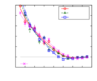
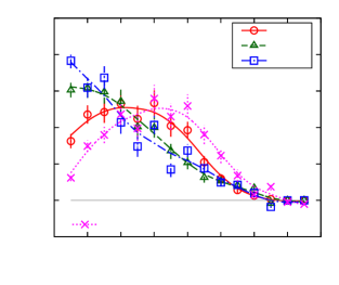
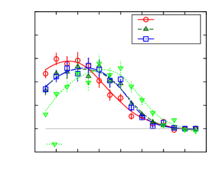
Figure 5: Optimal weights for 300 $\mu$m silicon (upper left) and 1 cm neon (upper right). Values are shown for $\beta\gamma=$ 1.00, 3.17 and 10.0. Optimal weights at $\beta\gamma=3.17$ are shown for 300, 600 and 1200 $\mu$m silicon (lower left); 1, 2 and 4 cm neon (lower right). All results are given for tracks with 15 hits ($i=1,\dots,15$). For comparison the optimal weights of the geometric mean are also shown (triangles down and crosses). The lines are drawn to guide the eye.

5 Weighted mean with different path lengths

In this study we assumed that the path lengths for each hit in the sensitive detector are the same. In case of real particle trajectories there is a variance due to bending in the magnetic field, placement of the detector units. The energy deposits can be corrected towards a reference path length. The distribution of energy deposit $\Delta$ depends on the velocity $\beta$ of the particle and the thickness of the traversed material $t$. To a good approximation, the most probable energy loss $\Delta_{p}$ and the full width of the distribution at half maximum $\Gamma_{\Delta}$ are [3]

$$\Delta_{p} =\xi\left[\ln\frac{2mc^{2}\beta^{2}\gamma^{2}\xi}{I^{2}}+0.2000-\beta^{2}-\delta\right]$$

$$\Gamma_{\Delta} =4.018\xi$$ (6)

where

$$\xi =\frac{K}{2}z^{2}\frac{Z}{A}\rho\frac{t}{\beta^{2}}$$

is the Landau parameter; $K=4\pi N_{A}r_{e}^{2}m_{e}c^{2}=0.307~{}075~{}\mathrm{MeV~{}cm^{2}/mol}$; $z$ is the charge of the particle in electron charge units; $Z$, $A$ and $\rho$ are the mass number, atomic number and the density of the material, respectively [8]. Let us consider the distribution of $y=\Delta/t$ values for a given particle, that is, at a fix $\beta$. The width of its distribution is independent of $t$ (Eq. (6)), while the most probable value $y_{p}$ scales with $t$ as

$$y_{p}(t)=y_{p}(t_{0})+\frac{K}{2}z^{2}\frac{Z}{A}\rho\frac{\ln(t/t_{0})}{\beta^{2}}$$

where $t_{0}$ denotes a fixed reference thickness. The slight $t$ dependence can be minimized by correcting each measurement to $y(t_{0})$. For that, $\beta$ can be estimated from $y$, obtained from the deposits without the above discussed path length correction.

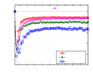
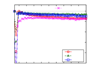
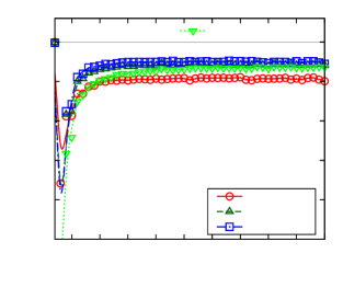
Figure 6: Performance of the optimized estimator. The ratio of the relative resolutions (weighted over simple truncated mean) is given as a function of number of hits on track $n$: for 300 $\mu$m silicon (upper left), and 1 cm neon (upper right), at various $\beta\gamma$ values; for silicon (lower left), and neon (lower right), at $\beta\gamma=3.17$ and various thicknesses. For comparison the performance of optimized weighted geometric mean is also shown (triangles down and crosses). Lines are drawn to guide the eye.

6 Results

Particle identification and yield extraction in the statistical sense are particularly difficult at those momenta where the differential energy losses of different type of particles are close. For hadrons, the pion-kaon resolution gets problematic above about 0.8 GeV/$c$, while for the pion-proton case it happens above about 1.6 GeV/$c$. Hence the relevant $\beta\gamma$ region is $1-10$.

In this work charged particles with $\beta\gamma=$ 1.00, 3.16 and 10.0 are studied, with number of hits $2-50$. Both semiconductor and gaseous detectors are investigated: for silicon thicknesses of 300, 600 and 1200 $\mu$m, while for neon with 1, 2 and 4 cm are chosen. For each study one million particles are used. (In order to speed up computation several million hits in 300 $\mu$m silicon and 1 cm neon were generated beforehand, for each $\beta\gamma$ settings, and later combined for longer path-length deposits.)

Comparisons of differential energy loss distributions and the estimators obtained via the simple truncated mean and the weighted arithmetic mean after optimization are shown in Fig. 4, in case of 6 hits on track.

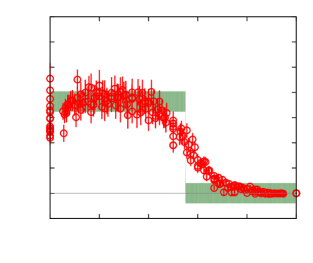
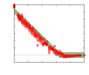
Figure 7: Optimal weights scaled with the number of hits ($n\cdot w_{i}$) as a function of normalized hit number $(i-1)/(n-1)$, if $4\leq n\leq 20$, at $\beta\gamma=3.17$. Values are shown for 300 $\mu$m silicon (left) and 1 cm neon (right). The shaded regions indicate a simple description of the weights: a combination of linear and constant functions with changes at 0.65 for silicon, and 0.55 for neon.

Optimal weights for 300 $\mu$m silicon and 1 cm neon are shown in Fig. 5-upper, for several $\beta\gamma$ values. Optimal weights for silicon and neon at $\beta\gamma=3.17$ are plotted in Fig. 5-lower, for several thicknesses. All results are given for tracks with 15 hits, $i=1,\dots,15$. The weights are remarkably independent of $\beta\gamma$ and material thickness for silicon, while some changes with increasing thickness are seen for neon. In case of silicon the hits $10\leq i\leq 15$ have very small, in some cases even negative weights, while the lowest deposits have the highest values. In case of 1 cm neon the hits $1\leq i\leq 8$ have roughly equal relevance, while the rest of the hits is not important. For comparison the optimal weights of the geometric mean are also shown. While for silicon there is good agreement with arithmetic mean weights, for neon the numbers somewhat differ but they show similar qualitative features.

The performance of the optimized estimator can be expressed as the ratio of the relative resolutions (weighted over simple truncated mean). These are shown as a function of number of hits on track at various $\beta\gamma$ values (Fig. 6-upper), and thicknesses (Fig. 6-lower). It is clear that there is substantial improvement for both silicon and neon, for all $\beta\gamma$ and thickness values. In case of few hits (e.g. $n=3$) the resolution decreased by 20-30% with respect to the simple truncation. Note that the improvement tends to a limiting value and the relative ratio is steadily below 1 for many hits. For comparison the performance of the optimized weighted geometric mean is also plotted. It essentially shows a behavior simular to that of the arithmetic mean, although with a better improvement at very low $n$ for neon.

6.1 Other considerations

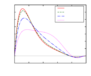
Detector and readout noise are more important for silicon since their magnitude is higher with respect to the energy deposit. Apart from the standard values (2 keV for silicon, 0.01 keV for neon), noise dependence of optimal weights was studied (Fig. 8). While higher values do not influence the weights for neon, in case of silicon at 10 keV their distribution starts to deform into a box distribution. This behavior can be understood: the addition of the Gaussian noise softens the lower leading edge of the energy deposit distribution (Fig. 1-left) and makes the lower values less important.

In a more complete detector simulation the effects of readout threshold (underflow, left truncation) and the upper limit of detector linearity (right censoring, overflow) should be taken into account. Still, this latter is likely not important since the highest deposits in any case will have low weights.

6.2 Universality, connections

While the list of weights as function of number of hits can be tabulated (see App. A), it would be much easier to find a simpler description. Optimal weights scaled with the number of hits ($n\cdot w_{i}$) as a function of normalized hit number $z\equiv(i-1)/(n-1)$ are plotted in Fig. 7, if $4\leq n\leq 20$. The dependence on the normalized hit number can be easily described as a combination of linear and constant functions. For silicon, with $z_{\text{Si}}\approx 0.65$,

$$n\cdot w_{i} =\begin{cases}2(z_{\text{Si}}-z)/z_{\text{Si}}^{2}&\text{if $z<z_{\text{Si}}$}\\ 0,&\text{otherwise}\end{cases}$$ (7)

while for neon, with $$z_{\text{Ne}}\approx 0.55$$,

$$n\cdot w_{i} =\begin{cases}1/z_{\text{Ne}}&\text{if $z<z_{\text{Ne}}$}\\ 0,&\text{otherwise}.\end{cases}$$ (8)

In case of many measurements, the optimal weights can be obtained using the energy deposit distribution, App. B gives a detailed derivation.

The simple functional forms described in Eqs. (7) and (8) have a deeper cause, namely it is strongly connected to the functional form of the deposit distribution. For detailed argumentation see App. C. If the density (Fig. 1) can be locally described by

• a power function, the local weights are zero;

• a product of exponential and power functions, the local weights are constant;

• a product of Gaussian and power functions, the local weights are linear in $z$.

This study was restricted to linear combination of measurements. It can be shown that while for semiconductor detectors the optimized weighted mean estimator may be further improved by using maximum likelihood methods, for gaseous detectors the simple (0%,55%) truncation (Eq. (8)) already gives excellent results (see App. D).

7 Conclusions

The estimation of differential energy loss for charged particles in tracker detectors was studied. It was shown that the simple truncated mean method can be generalized to the linear combination of the energy deposit measurements. The optimized weights are rather independent of particle momentum and material thickness, allowing for a robust estimation. Weighted arithmetic and geometric means result in better particle separation power for both semiconductor and gaseous detectors. Further inspections showed that weights are deeply connected to corresponding energy deposit distribution, allowing for a simple universal description of weights as function of number of hits.

Appendix A Optimal weights in case of few measurements

The obtained weights for 300 $\mu$m silicon and 1 cm neon, at $\beta\gamma=3.17$, in case of hit numbers $2\leq n\leq 9$ are shown in Tables 1 and 2, respectively. Errors indicate the sensitivity corresponding to 1% increase of the relative resolution of the estimator.

Appendix B Optimal weights in case of many measurements

A random variable $x$ is described by the probability density function $f(x)$ and cumulative distribution function $F(x)=\int_{-\infty}^{x}f(x^{\prime})dx^{\prime}$. During an observation $f$ is sampled $n$ times, these measurements are rearranged to increasing order ($x_{i}\leq x_{i+1}$, $i=1,2,\dots,n$). We are interested in the means $m_{i}$ and covariance $V_{ij}$ of the ordered samples in the continuous limit ($n\gg 1$).

B.1 Means and covariance of measurements

The probability density that $x_{i}$ is the $i$th measurement

$$p(x_{i})=\frac{n!}{(i-1)!(n-i)!}F(x_{i})^{i-1}f(x_{i})[1-F(x_{i})]^{n-i}.$$

It is easier to work with $-\log p$, since its minimum gives the most probable value $\overline{x_{i}}$. In the Gaussian approximation the mean $m_{i}=\overline{x_{i}}$ and its variance $V_{ii}$ is also calculable. If $1<i<n$, then the factors containing $F$ already constrain well enough the position of $m_{i}$, hence $f(x_{i})$ can be approximated by a constant:

$$p(x_{i})\approx\frac{n!}{(i-1)!(n-i)!}F(x_{i})^{i-1}[1-F(x_{i})]^{n-i}.$$ (9)

At $x_{i}=m_{i}$

$$[-\log p(x)]^{\prime} =0, 1/V_{ii} =[-\log p(x)]^{\prime\prime}.$$

By solving the equation on the left, we get

$$F(m_{i}) =\frac{i-1}{n-1}, V_{ii} =\frac{(i-1)(n-i)}{(n-1)^{3}f^{2}(m_{i})}.$$ (10)

Note again that the above approximations are valid only for $1<i<n$. (For the lowest and highest measurements we would get $m_{1}=-\infty$, $m_{n}=\infty$, and $\sigma_{1}^{2}=\sigma_{n}^{2}=\infty$.)

The probability density that $x_{i}$ and $x_{j}$ are the $i$th and $j$th measurements ($i\leq j$), respectively,

$$p(x_{i},x_{j})=\frac{n!}{(i-1)!(j-i-1)!(n-j)!}\cdot\\ \cdot F(x_{i})^{i-1}[F(x_{j})-F(x_{i})]^{j-i-1}[1-F(x_{j})]^{n-j}.$$

Similarly to Eq. (9), by assuming $1<i<j<n$, we have omitted the factors $f(x_{i})$ and $f(x_{j})$.

Close to its minimum $p(x_{i},x_{j})$ can be approximated by a multivariate normal distribution. At the minimum ($x_{i}=m_{i}$ and $x_{j}=m_{j}$) the correlation coefficient is

$$\rho_{ij}={\frac{\partial^{2}\log p}{\partial x_{i}\partial x_{j}}}\;\Biggl{/}{\sqrt{\frac{\partial^{2}\log p}{\partial x_{i}^{2}}\frac{\partial^{2}\log p}{\partial x_{j}^{2}}}}.$$

The partial derivatives are

$$\frac{\partial^{2}\log p}{\partial x_{i}\partial x_{j}} =(n-1)^{2}\frac{j-i-1}{(j-i)^{2}}f(m_{i})f(m_{j}))$$

$$\begin{split}\frac{\partial^{2}\log p}{\partial x_{i}^{2}}&=\frac{n-1}{j-i}f^{\prime}(m_{i})-\\ &-(n-1)^{2}\frac{(j-i)(j-1)-(i-1)}{(i-1)(j-i)^{2}}f^{2}(m_{i})\end{split}$$

$$\begin{split}\frac{\partial^{2}\log p}{\partial x_{j}^{2}}&=-\frac{n-1}{j-i}f^{\prime}(m_{j})-\\ &-(n-1)^{2}\frac{(j-i)(n-i)-(n-j)}{(n-j)(j-i)^{2}}f^{2}(m_{j}).\end{split}$$

In the $n\gg 1$ limit the coefficients of $f^{\prime}$ can be neglected if compared to the ones of the $f^{2}$ terms. Similarly the nominators of the coefficient of $ff$ in all three cases can be simplified by neglecting the terms $1$, $(i-1)$ and $(n-j)$, respectively:

$$\frac{\partial^{2}\log p}{\partial x_{i}\partial x_{j}} \approx(n-1)^{2}\frac{1}{j-i}f(m_{i})f(m_{j})$$

$$-\frac{\partial^{2}\log p}{\partial x_{i}^{2}} \approx(n-1)^{2}\frac{(j-1)}{(i-1)(j-i)}f^{2}(m_{i})$$

$$-\frac{\partial^{2}\log p}{\partial x_{j}^{2}} \approx(n-1)^{2}\frac{(n-i)}{(n-j)(j-i)}f^{2}(m_{j}).$$

With that the correlation coefficient is

$$\rho_{ij}=\sqrt{\frac{(i-1)(n-j)}{(n-i)(j-1)}}.$$

Note that $\rho_{ij}$ does not depend on $f$. The covariance of the $i$th and $j$th measurements ($i\leq j$) is

$$V_{ij}=\rho_{ij}\sqrt{V_{ii}V{jj}}=\frac{(i-1)(n-j)}{(n-1)^{3}f(m_{i})f(m_{j})}.$$ (11)

The expression gives nicely back the variance ($i=j$) already obtained in Eq. (10)-right.

B.2 Optimal weights

With the vector of means $m_{i}$ (Eq. (10)-left) and the covariance matrix $V_{ij}$ (Eq. (11)), the optimal weights are calculable. In the high $n$ limit, we can consider the following continuous variables

$$a \equiv\frac{i-1}{n-1}, b \equiv\frac{j-1}{n-1}, 0<a,b<1.$$

The means and covariance in this variables are

$$m(a) =F^{-1}(a)$$

$$V(a,b) =\operatorname{min}(a,b)[1-\operatorname{max}(a,b)]m^{\prime}(a)m^{\prime}(b).$$

On the analogy of $m=Vw$ there is a Friedholm integral equation of the first kind for $w$

$$m(a)=\int_{0}^{1}V(a,b)w(b)\mathrm{d}b=\\ =\int_{0}^{1}\operatorname{min}(a,b)[1-\operatorname{max}(a,b)]m^{\prime}(a)m^{\prime}(b)w(b)\mathrm{d}b.$$

It can be written in the form

$$g(a)=\int_{0}^{1}K(a,b)y(b)\mathrm{d}b$$

where

$$g(a)=\frac{m(a)}{m^{\prime}(a)},\qquad y(b)=m^{\prime}(b)w(b)$$

$$K(a,b)=\operatorname{min}(a,b)[1-\operatorname{max}(a,b)].$$

The kernel $K$ is a special one

$$g(a)=\int_{0}^{a}(1-a)by(b)\mathrm{d}b+\int_{a}^{1}a(1-b)y(b)\mathrm{d}b$$

$$g^{\prime}(a)=-\int_{0}^{a}by(b)\mathrm{d}b+\int_{a}^{1}(1-b)y(b)\mathrm{d}b$$

The equation can be solved by two consecutive derivations in $$a$$ giving the result

$$g^{\prime\prime}(a)=-y(a).$$

In summary the optimal weights $w$ in the continuous variable $a$ are

$$w=-\frac{1}{m^{\prime}}\left(\frac{m}{m^{\prime}}\right)^{\prime\prime}.$$ (12)

With the energy loss $m$ as variable, for a weight at $F(m)$

$$w[F(m)]=-\frac{f^{\prime}}{f}+m\left(\frac{f^{\prime}}{f}\right)^{2}-m\frac{f^{\prime\prime}}{f}=\\ =-\left[m(\log f)^{\prime}\right]^{\prime}.$$ (13)

With help of this exact result (Eq. (13)), the optimal weights scaled with the number of hits ($n\cdot w_{i}$) as a function of normalized hit number $z\equiv(i-1)/(n-1)$ are shown in Fig. 8, at $\beta\gamma=3.17$, if $n$ is big.

The minimum of the relative resolution of the weighted average is

$$\frac{1}{\sqrt{\int_{0}^{1}mw}}=\frac{1}{\sqrt{-\int_{0}^{1}\frac{m}{m^{\prime}}\left(\frac{m}{m^{\prime}}\right)^{\prime\prime}}}.$$

Figure 8: Optimal weights scaled with the number of hits ($n\cdot w$) as a function of normalized hit number $(i-1)/(n-1)$, if $n$ is big, at $\beta\gamma=3.17$. Values are shown for 300 $\mu$m silicon (left) and 1 cm neon (right), both with several noise settings.

Appendix C Irrelevant and equally relevant measurements

In the continuous limit we can find probability distribution functions $f$ with special characteristics, by solving Eq. (12).

The ordered measurements are irrelevant if $w=0$. The condition $1/m^{\prime}=0$ would give $f=0$, a meaningless unphysical solution. On the other hand if

$$\left(\frac{m}{m^{\prime}}\right)^{\prime\prime}=0\qquad\Rightarrow\qquad m(z)=\left(\frac{z+d/(b+1)}{a}\right)^{1/(b+1)}$$

$$f(m)=\frac{1}{m^{\prime}(z)}=a\cdot m^{b}.$$ (14)

Hence measurements from distributions with power functions should be neglected, their optimal weights are zero.

The ordered measurements are equally relevant if

$$w=-\frac{1}{m^{\prime}}\left(\frac{m}{m^{\prime}}\right)^{\prime\prime}=c=const>0.$$

The equation

$$-f[m(z)]\frac{\partial^{2}\left(m(z)f[m(z)]\right)}{\partial z^{2}}=c$$

can be solved by resolving the composition $$f\circ m$$, giving

$$f(m)=a\cdot m^{b}\exp(-c\cdot m),$$

which is the product of a power and an exponential function (compare with Fig. 1-right and Fig. 7-left, the case of neon). Note that $c=0$ indeed gives back the result in Eq. (14). It can be shown that weights are a linear function of $z$ if $f(m)$ is the product of a power and a Gaussian function (compare with Fig. 1-left and Fig. 7-left, the case of silicon).

The distribution of energy loss $f(\Delta)$ examined in this study has a $1/\Delta^{2}$ behavior for large energy deposits due to Coulomb excitations. (The Landau distribution, which is often used to model and approximate energy loss, also has a $1/\Delta^{2}$ power-law tail.) This is why we got small optimal weights for the upper measurements. It is also the fundamental cause for the success of the classical truncated mean method.

Appendix D Connection to maximum likelihood estimation

In this work the optimization of differential energy loss estimation was confined to the linear combination of the measurements, or of a monotonic function of the measurements. Are there cases when this relatively simple prescription is close to the performance of a, supposedly more powerful, maximum likelihood estimation?

Let us assume that the scale of energy loss distribution is characterized by the most probable deposit $y_{P}$, such that the probability of a deposit $y_{i}$ is given by

$$\frac{y_{0}}{y_{P}}f\left(y_{i}\frac{y_{0}}{y_{P}}\right)$$

where $$f y_{0} n$$ is a universal function and is constant. In that case the likelihood associated to a track with hits is

$$P=\prod_{i=1}^{n}\frac{y_{0}}{y_{P}}f\left(y_{i}\frac{y_{0}}{y_{P}}\right)$$

and

$$-\log P=\sum_{i=1}^{n}\left[\log\frac{y_{P}}{y_{0}}-\log f\left(y_{i}\frac{y_{0}}{y_{P}}\right)\right].$$

Its value is extremum if the derivative is zero, giving

$$y_{p}=y_{0}\sum_{i=1}^{n}\frac{y_{i}}{n}\cdot(-\log f)^{\prime}\left(y_{i}\frac{y_{0}}{y_{P}}\right).$$

The most probable value $y_{P}$ can be obtained by a simple linear combination of measurements if, for an interval around $y_{i}$, the function $(-\log f)^{\prime}$ behaves as

$$(-\log f)^{\prime}(y)=c_{i}-b_{i}/y$$

where $$c_{i} b_{i}$$ and are local constants. With this

$$y_{P}=\frac{y_{0}}{\sum_{i=1}^{n}(1+b_{i})}\sum_{i=1}^{n}c_{i}y_{i}.$$

The corresponding functional form is

$$f(y)=a\cdot y^{b}\exp(-c\cdot y)$$

that exactly matches the form found for neon (see Fig. 1-right and App. C).

In summary we can say that while for semiconductor detectors the optimized weighted mean estimator may be further improved with maximum likelihood methods, for gaseous detectors the simple (0%,55%) truncation already gives excellent results.

References

• [1] O. Ullaland, Update in particle identification, Nucl. Phys. Proc. Suppl. 125 (2003) 90–99. doi:10.1016/S0920-5632(03)90972-8.
• [2] H. Yamamoto, dE/dx particle identification for collider detectorsarXiv:hep-ex/9912024.
• [3] H. Bichsel, Straggling in thin silicon detectors, Rev. Mod. Phys. 60 (1988) 663–699. doi:10.1103/RevModPhys.60.663.
• [4] H. Bichsel, Inelastic electronic collision cross sections for monte carlo calculations, Nucl. Instrum. Meth. B52 (1990) 136. doi:10.1016/0168-583X\%2890\%2990581-E.
• [5] H. Bichsel, A method to improve tracking and particle identification in TPCs and silicon detectors, Nucl. Instrum. Meth. A562 (2006) 154–197. doi:10.1016/j.nima.2006.03.009.
• [6] R. C. Fernow, Introduction to experimental particle physics, Cambridge University Press, 1986, pages 253-255.
• [7] C. Grupen, B. Shwartz, H. Spieler, Particle Detectors, 2nd Edition, Cambridge University Press, 2008, pages 278-280.
• [8] K. Nakamura, et al., Review of particle physics, J.Phys.G G37 (2010) 075021. doi:10.1088/0954-3899/37/7A/075021.