On particle trajectories in linear deep-water waves
Abstract.
We determine the phase portrait of a Hamiltonian system of equations describing the motion of the particles in linear deep-water waves. The particles experience in each period a forward drift which decreases with greater depth.
Key words and phrases:
Linear deep-water waves; Particle trajectory; Phase portrait2000 Mathematics Subject Classification:
76B15, 34C25, 35Q35.1. Introduction
The motion of water particles under the waves which advance across the water is a classical problem in this field. Watching the sea it is oft possible to trace a wave as it propagates on the water’s surface, but what one observes traveling across the sea is not the water but a wave pattern. Although the wave travels from one place to another, the substance through which it travels moves very little. As the wave advances across the water and can be followed for a long way, a typical water particle moves slightly up and down, forward and backward as the wave passes it. If an object hovered in the water, like a water particle, its motion would be synchronized with that of a floating object lying on the water’s surface, with its orbit diminishing with the distance from the surface. As waves generated by wind in an area move towards a region where the wind has ceased, we observe swell-long crested two-dimensional waves approaching a smooth sinusoidal shape and moving over long distances. Deep-water waves are modelled mathematically as periodic two-dimensional waves in water of infinite depth. The motion of the water particle in the fluid below swell is of great interest. The classical description of these particle paths is obtained within the framework of linear water wave theory [1, 15, 16, 23, 24, 25, 29, 30]: all water particles trace a circular orbit, the diameter of which decreases with depth so that the orbital motion practically ceases at depth equal to one-half the wavelength. These features have important practical consequences. For example, a submarine at a depth below half a wavelength would hardly notice the motion of the surface wave, for this reason submarines dive during storms in the open sea.
The only known explicit solution with a non-flat free surface of the governing equations for gravity water waves is Gerstner’s wave [17]: a deep-water wave solution for which all particle paths are circles of diameters decreasing with the distance from the free surface (see the discussion in [2, 3]). Due to the mathematical intractability of the governing equations for water waves, for irrotational water waves (Gerstner’s wave has a peculiar nonvanishing vorticity) the classical approach [15, 20, 23, 24, 28, 29, 30] relies on analyzing the particle motion after linearization of the governing equations. However, even within the linear water wave theory, the ordinary differential equations system describing the motion of the particles is nevertheless nonlinear and explicit solutions of this system are not available, but qualitative features of the underlying flow are known [6, 9, 10, 11, 21, 26, 27, 33] and could possibly lead to a confirmation of the features we prove here, within the confines of linear water waves (see [4]).
In this paper we show that for linear deep-water wave no particle trajectory is actually closed, unless the free surface is flat. Each trajectory involves over a period a backward/forward movement of the particle, and the path is an elliptical arc with a forward drift. Support for this conclusion is given by the analysis of the average flow of energy within linear water wave theory (see [23]): due to the passage of a periodic surface wave, the water particles in the fluid experience on average a net displacement in the direction in which the waves are propagating, termed Stokes drift [31] (see the discussion in [34]). This result was first obtained in [13] for gravity waves and [19] for capillary and capillary-gravity water waves. This results have been improved in [4, 9, 18] in the case of irrotational waves by describing the exact geometry of the actual particle paths. For gravity deep-water waves we reconfirm herein the results of [13], but our analysis is more precise and uses only elementary analysis methods. The work is structured as follows: we recall first the governing equations for water waves and give the exact solutions of the linearised problem. Our major contribution, in Section 3, is a precise analysis of the phase portrait of a Hamiltonian system associated to the particle motion. This is the key point in determining the trajectories of the water particles.
2. Preliminaries
In this section we recall the governing equations for the propagation of two-dimensional gravity deep-water waves and we present their linearization (for a more detailed discussion we refer to [23]).
2.1. The governing equations
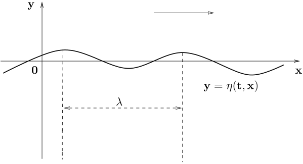
We consider a two-dimensional inviscid incompressible fluid in a constant gravitational field. To describe the waves propagation we consider a cross section of the flow that is perpendicular to the crest line with Cartesian coordinates , the -axis pointing vertically upwards and the -axis being the direction of wave propagation (see Figure 1). Let be the velocity field and the equation of the free surface with mean water level zero is with .
Constant density (homogeneity) is a physically reasonable assumption for gravity waves [23], and it implies the equation of mass conservation
| (2.1) |
Under the assumption of inviscid flow the equation of motion is Euler’s equation
| (2.2) |
where denotes the pressure and is the gravitational constant of acceleration. The free surface decouples the motion of the water from that of the air, a fact that is expressed in [23] by the dynamic boundary condition
| (2.3) |
if we neglect surface tension, where is the (constant) atmospheric pressure. Since the same particles always form the free surface, we also have the kinematic boundary condition
| (2.4) |
The boundary condition at the bottom
| (2.5) |
expresses the fact that at great depths there is practically no motion. Summarising, the governing equations for water waves are encompassed by the nonlinear free-boundary problem
| (2.6) |
 |
An important category of flows are those of zero vorticity (irrotational flows), characterized by the additional assumption
| (2.7) |
The vorticity of a flow, , measures the local spin or rotation of a fluid element so that in irrotational flows the local whirl is completely absent. Relation (2.7) ensures the existence of a velocity potential defined up to a constant via
In view of (2.1), is a harmonic function, i.e. so that the methods of complex analysis become available for the study of irrotational flows.
Concerning the physical relevance of irrotational water flows, field evidence indicates that for waves entering a region of still water the assumption of irrotational flow is realistic [25]. Moreover, as a consequence of Kelvin’s circulation theorem [1], a water flow that is irrotational initially has to be irrotational at all later times. It is thus reasonable to consider that water motions starting from rest will remain irrotational at later times. Nonzero vorticity is the hallmark of the interaction between waves and non-uniform currents cf. [10] and [12, 22]. The most important example of rotational flows are tidal currents cf. the discussion in [5, 32], but the assumption of constant vorticity can not be accomodated within the framework of deep-water flows. However, we consider herein irrotational gravity waves.
2.2. Linear water waves
The problem (2.6) is nondimensionalised using a typical wavelength and a typical amplitude of the wave . We define the set of nondimensional variables
combined with the scaling
Setting the constant water density , the pressure in the new nondimensional variables is
with the nondimensional pressure variable measuring the deviation from the hydrostatic pressure distribution. We obtain the following boundary value problem in nondimensional variables
| (2.8) |
The linearized problem is now obtained by letting in (2.8). In the limit we arrive at
| (2.9) |
It is worth noticing that the regularity results on the streamlines for water waves obtained in the recent papers [27] and [8] ensure that good approximate properties hold.
Looking for solutions of (2.9) representing waves traveling at speed , we impose that all functions and have an -dependence in the form of . Furthermore, one seeks even periodic functions of period one, the evenness expressing the symmetry of the surface wave: it is known, cf. [6] and [7, 14] that a gravity surface traveling wave whose profile is monotone between the crests and troughs has to be symmetric about the crest. Thus, we are led to the fundamental Fourier mode Ansatz
For this specific the problem (2.9) has the solution
whereby the constant and the function are given by
Marking the variables of this nondimensional solution by tildes, we recover the physical variables by the backward transformation
Defining the wavenumber and the frequency by
where we finally obtain that the tupel
| (2.10) |
is a solution of the linearised deep-water wave problem. Note that in the physical variables the speed of the wave in (2.10) is
3. Particle trajectories
In this last section we study the trajectories of the water particles in the linear wave (2.10). First of all, we note that a fluid particle must satisfy the following equations
so that, in view of (2.10), the motion of the particle is described by the system
| (3.1) |
with initial data We use herein the shorthand
| (3.2) |
The right-hand side of the differential system (3.1) is smooth so that the existence of a unique local smooth solution is ensured the Picard-Lindelöf theorem. Without actually solving (3.1) we would like to display the principal features of the solution. To study the exact solutions to (3.1) it is convenient to re-write the system in a moving, and we define therefore the variables
| (3.3) |
With this notation (3.1) is equivalent to the following problem
| (3.4) |
with In order to determine the phase portrait corresponding to (3.4), we take into consideration the property of (3.4) of being a Hamiltonian system. Indeed, setting
| (3.5) |
we re-express problem (3.4) as follows
| (3.6) |
Since is constant on solutions of (3.6), we are left to determine the level curves of the function . In [13] the authors studied the phase portrait of (3.6) approximately, by using Morse’s lemma. A precise analysis allows us to determine herein the phase portrait of the Hamiltonian system of equations describing the motion of the particles in linear deep-water waves by using only elementary methods.
Note that is periodic in and even with respect to the same variable. Therefore, the level curves of are determined by the level sets of the restriction where . Furthermore, it is not difficult to see that the equation has a unique solution
meaning that is the unique stationary solution of (3.6) within Moreover, is located on the level curve with given by
We make now a crucial observation. Let be given with for some In view of it must hold that
with The definition domain of consists of all the points which satisfy the inequalities
| (3.7) |
Hence for all and we are left to determine the definition domain of the function , that is to solve the inequality (3.7). The first important result of this paper is the following theorem which gives a precise description of the phase curves of (3.6):
 |
Theorem 3.1.
Given , there exists a function such that for all More precisely, there exists a unique such that
-
If , then
Moreover, the minimum of belongs to the interval
-
If , there exist positive real numbers with such that
Moreover, is bijective and decreasing, whereas is bijective and increasing.
Additionally, we have
-
is bijective and decreasing;
-
is bijective and decreasing;
-
is bijective and increasing;
-
as
The functions mentioned above are real analytic in the interior of their definition domain (excepting which is real analytic only on ).
Remark 3.2.
Having proved Theorem 3.1, the phase portrait is complete (see Figure 2). Note that by , we know that the phase curves parametrised by flatten out as The motion along the phase curves is determined by the fact that
provided The phase portrait also discloses that the stationary solution is a saddle node for (3.5). Solutions starting in a point located on a separatrix (one of the level curves containing ) are attracted by provided On the other hand, if they tend to infinity.
Proof of Theorem 3.1.
Let We observe first that the equation is always solvable in Indeed, it is equivalent to the following relation
Clearly, the function is strictly decreasing and, moreover,
| (3.8) |
Whence, there exists a unique real number such that Consequently, all phase curves of (3.6) intersect the line exactly once, that is at
A simple calculation shows that
and we infer from the implicit function theorem that is real analytic and, additionally
| (3.9) |
This implies that is strictly decreasing. Due to (3.8), we conclude that is bijective. Differentiating at we observe that
| (3.10) |
Let us now compare the value of at the threshold value , where the monotonicity changes, to , the larges value can take in order to remain in the definition domain of . We recover , since
Analogously, we have that if and only if Since is the (positive) maximum of and , we conclude that
for all Particularly, if then for all Moreover, taking into account that we conclude that for all
On the other hand, if then and there exist precisely two points with the property that , . By (3.10) we have that , and we infer from the implicit function theorem that is strictly decreasing, while is strictly increasing. We have use the fact that both and verify, due to , relation (3.9). With this, the assertions and are immediate.
Knowing the phase curves the particle trajectories in the linear wave (2.10) are given, via (3.3), by
| (3.11) |
For physical reasons realistic particle paths are bounded. Thus, the critical point must at least lie above the typical height of the wave. Since the mean surface level is zero and the amplitude is a crest has coordinate Since the coordinate of is , we must thus impose that that is
| (3.12) |
This is the only condition which has to be imposed for (2.10) to be a realistic model of water waves of infinite depth, wave number and small amplitude . This is an improvement compared to [13], because we do not have to to make sure that the separatrix intersects the the line only once; this is in our case a conclusion of studying the phase portrait of (3.6).
We describe now the trajectory of the water particle in the fluid. We may consider the orbit of a particle which starts at the lowest point (corresponding to the line in the phase-portrait). This trajectory corresponds to the solution of (3.6) which starts at Furthermore, we denote by the time needed for to reach the line Indeed, from thre first equation of (3.6) we have for located beneath that is under the separatrix, that
| (3.13) |
hence depends only of . Let us observe the evolution of the particle as Since we find see from (3.6) that
Also, from the phase portrait of (3.6), we see that the hight of the particle reaches its initial value for the first time when What we still have to establish is the sign of
 |
Since
we find from (3.13) that
with In view of we conclude that the water particle experiences a forward drift equal to
Clearly, by the definition of we see that the drift decreases with depth and, in the limit , the forward drift vanishes
Whence, we have shown that:
Theorem 3.3.
The particle paths in the linear water wave (2.10) are not closed. There exists a forward drift over a period, and this drift decreases with depth.
References
- [1] Acheson, D. J.: Elementary Fluid Dynamics, The Clarendon Press, Oxford Univ. Press, New York, 1990.
- [2] Constantin, A.: On the deep water wave motion, J. Phys. A, 34 (2001), 1405–1417.
- [3] Constantin, A.: Edge waves along a sloping beach, J. Phys. A, 34 (2001), 9723–9731.
- [4] Constantin, A.: The trajectories of particles in Stokes waves, Inventiones Mathematicae, 166 (2006), 523–535.
- [5] Constantin, A.: Two-dimensionality of gravity water flows of constant nonzero vorticity beneath a surface wave train, Eur. J. Mech. B Fluids, 30 (2011), 12–16.
- [6] Constantin, A. & Escher, J.: Symmetry of steady periodic surface water waves with vorticity, J. Fluid Mech., 498 (2004), 171–181.
- [7] Constantin & Escher, J.: Symmetry of steady deep-water waves with vorticity, European J. Appl. Math., 15 (2004), 755–768.
- [8] Constantin & Escher, J.: Analyticity of periodic traveling free surface water waves with vorticity, Ann. of Math., 173 (2011), 559–568.
- [9] Constantin, A. & Strauss, W. : Pressure beneath a Stokes wave, Comm. Pure Appl. Math., 63 (4) (2010), 533-557.
- [10] Constantin, A. & Strauss, W. : Exact steady periodic water waves with vorticity, Comm. Pure Appl. Math., 57 (2004), 481–527.
- [11] Constantin, A., Sattinger, D. & Strauss, W.: Variational formulations for steady water waves with vorticity, J. Fluid Mech., 548 (2006), 151–163.
- [12] Constantin, A. & Villari, G.: Particle trajectories in linear water waves, J. Math. Fluid Mech., 10 (2008), 1–18.
- [13] Constantin, A., Ehrnström, M. & Villari, G.: Particle trajectories in linear deep-water waves, Nonlinear Analysis: Real World Application , 9 (2008), 1336–1344.
- [14] Constantin, A., Ehrnström, M. & Wahlén, E.: Symmetry of steady periodic gravity water waves with vorticity, Duke Math. J. , 140 (2007), 591–603.
- [15] Crapper, G. D.: Introduction to Water Waves, Ellis Horwood Ltd., Chichester, 1984.
- [16] Debnath, L.: Nonlinear Water waves, Academic Press, Inc., Boston, MA, 1994.
- [17] Gerstner, F.: Theorie der Wellen samt einer daraus abgeleiteten Theorie der Deichprofile, Ann. Phys., 2 (1809), 412–445.
- [18] Henry, D.: The trajectories of particles in deep-water Stokes waves, Int. Math. Res. Not. Art. ID 23405 (2006), 1–13.
- [19] Henry, D.: Particle trajectories in linear periodic capillary and capillary-gravity deep-water waves, J. Nonlinear Math. Phys. 14(1) (2007), 1–7.
- [20] Henry, D.: On Gerstner’s water wave, J. Nonlinear Math. Phys. 15 (2008), 87–95.
- [21] Hur, V.: Global bifurcation theory of deep-water waves with vorticity, SIAM J. Math. Anal., 37 (2006), 1482–1521.
- [22] Ionescu-Kruse, D.: Particle trajectories in linearized irrotational shallow water flows, J. Nonlinear Math. Phys. 15 (2008), 13–27.
- [23] Johnson, R. S.: A Modern Introduction to the Mathematical Theory of Water Waves, Cambridge Univ. Press, Cambridge, 1997.
- [24] Lamb, J.: Hydrodynamics, Cambridge Univ. Press, Cambridge, 1895.
- [25] Lighthill, J.: Waves in Fluids, Cambridge Univ. Press, Cambridge, 1978.
- [26] Matioc, A. V.: On particle trajectories in linear water waves, Nonlinear Analysis: Real World Applications, 11 (2010), 4275-4284.
- [27] Matioc, B. V.: On the regularity of deep-water waves with general vorticity distributions, to appear in Quart. Appl. Math..
- [28] Milne-Thomson, L. M.: Theoretical Hydrodynamics, The Macmillan Co., London, 1938.
- [29] Sommerfeld, A.: Mechanics of Deformable Bodies, Academic Press, Inc., Boston, MA, 1950.
- [30] Stoker, J. J.: Water Waves. The Mathematical Theory with Applications, Interscience Publ. Inc., New York, 1957.
- [31] Stokes, G. G.: On the theory of oscillatory waves, Trans. Cambridge Phil. Soc., 8 (1847), 441-455.
- [32] Teles da Silva, A.F. & Peregrine, D. H.: Steep, steady surface waves on water of finite depth with constant vorticity, J. Fluid Mech., 195 (1988), 281–302.
- [33] Toland, J.F: Stokes waves, Topol. Methods Nonlinear Anal., 7 (1996), 1–48.
- [34] Yih, C.-S.: The role of drift mass in the kinetic energy and momentum of periodic water waves and sound waves, J. Fluid Mech, 331 (1997), 429 -438.