Bondi-Hoyle Accretion onto Magnetized Neutron Star

Abstract

Axisymmetric MHD simulations are used to investigate the Bondi-Hoyle accretion onto an isolated magnetized neutron star moving supersonically (with Mach number of 3) through the interstellar medium. The star is assumed to have a dipole magnetic field aligned with its motion and a magnetospheric radius $R_{\rm m}$ less then the accretion radius $R_{\rm BH}$, so that the gravitational focusing is important. We find that the accretion rate to a magnetized star is smaller than that to a non-magnetized star for the parameters considered. Close to the star the accreting matter falls to the star’s surface along the magnetic poles with a larger mass flow to the leeward pole of the star. In the case of a relatively large stellar magnetic field, the star’s magnetic field is stretched in the direction of the matter flow outside of $R_{\rm m}$ (towards the windward side of the star). For weaker magnetic fields we observed oscillations of the closed magnetosphere frontward and backward. These are accompanied by strong oscillations of the mass accretion rate which varies by factors $\sim 3$. Old slowly rotating neutron stars with no radio emission may be visible in the X-ray band due to accretion of interstellar matter. In general, the star’s velocity, magnetic moment, and angular velocity vectors may all be in different directions so that the accretion luminosity will be modulated at the star’s rotation rate.

1 Introduction

Accretion onto a supersonically moving star is an important astrophysical process which has been studied theoretically and with simulations over many years (review by Edgar 2004). This type of accretion has applications in many areas. For example, the accretion by a compact star in a binary system where the gas supply is from a stellar wind or from a common envelope (Petterson 1978; Taam and Sandquist 2000); and flows in regions of star formation (Bonnell et al. 2001; Edgar and Clarke 2004).

Supersonic accretion of a pressureless fluid onto a gravitating center was investigated analytically by Hoyle and Lyttleton (1939) and an analytic solution was found by Bisnovatyi-Kogan et al. (1979). Later, Bondi and Hoyle (1944) developed a model including the fluid pressure. The Bondi-Hoyle model gives an explicit prediction for the accretion rate.

Supersonic accretion has been studied using numerical hydrodynamic simulations by Ruffert (Ruffert, 1994a; Ruffert and Arnett, 1994; Ruffert, 1994b). He studied the flow of gas past an accretor of varying sizes. For small accretors, the accretion rates obtained were in broad agreement with theoretical predictions. Accretion of matter to a nonmagnetized gravitating center was investigated by Bisnovatyi-Kogan & Pogorelov (1997). Pogorelov, Ohsugi, & Matsuda (2000) studied the Bondi-Hoyle accretion flow and its dependence on parameters but also for a nonmagnetized center.

Here, we investigate Bondi-Hoyle accretion to magnetized stars in application to the accretion of the interstellar medium (ISM) onto Isolated Old Neutron Stars (IONS). These slowly rotating neutron stars may be visible due accretion of the interstellar medium. These stars may have dynamically important magnetic fields. We use axisymmetric magnetohydrodynamics simulations to model the accretion onto the star. Earlier, we investigated cases of supersonic motion of strongly magnetized stars through the ISM in cases of slow rotation (Toropina at all 2001; hereafter T01) and fast rotation in the propeller regime (Toropina, Romanova, Lovelace 2006; hereafter T06). In these cases the magnetospheric radius is greater then accretion radius $R_{\rm m}\geq R_{\rm BH}$ and gravitational focusing is not important. Both cases correspond to magnetars with magnetic field $B\gtrsim 10^{14}$ G.

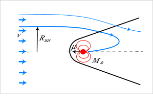
Figure 1: Sketch of the Bondi-Hoyle accretion onto a supersonically moving magnetized star. The thick black line is the shock wave and the red lines are the field lines of the star.

The present simulations are analogous to those in T01 and T06. However, here the star has a more typical neutron star magnetic field, $B\sim 10^{10}-10^{12}$ G. The magnetospheric radius is less then the accretion radius and gravitational focusing is important. A star gathers matter from the region inside the accretion radius.

Sections 2 and 3 describe the physical situation and simulation model. In Sec. 4 we discuss the results of our simulations. In Sec. 5 we apply our results to more realistic neutron stars. Conclusions are given in Sec. 6.

2 Physical Model

A non-magnetized star moving through the ISM captures matter gravitationally from the accretion or Bondi-Hoyle radius

$$R_{\rm BH}={2GM\over c_{s}^{2}+v^{2}}\approx 3.8\times 10^{12}{M_{1.4}\over v_{100}^{2}}~{}{\rm cm}~{},$$

where $v_{100}\equiv v/(100~{}{\rm km/s})$ is the normalized velocity of the star, $c_{s}$ the sound speed of the undisturbed ISM, and $M_{1.4}\equiv M/(1.4M_{\odot})$ is the normalized mass of the star. The mass accretion rate at high Mach numbers ${\cal M}\equiv v/c_{s}>>1$ was derived by Hoyle and Lyttleton (1939),

$$\dot{M}_{\rm HL}=4\pi(GM)^{2}{\rho\over v^{3}}\approx 7.3\times 10^{8}{n\over v_{100}^{3}}M_{1.4}^{2}~{}{\rm\frac{g}{s}}~{},$$

where $\rho$ is the mass-density of the ISM and $n=n/{1~{}{\rm cm}^{-3}}$ is the normalized number density.

The Hoyle-Lyttleton model neglects the fluid pressure as mentioned. Later, Bondi and Hoyle (1944) extended the analysis to include the pressure. A more general formula for arbitrary Mach numbers ${\cal M}=v/c_{s}$ was proposed by Bondi (1952),

$$\dot{M}_{\rm BH}=\pi R_{\rm BH}^{2}\rho v=4\pi\alpha(GM)^{2}{\rho\over(v^{2}+c_{s}^{2})^{3/2}}~{},$$

where the coefficient $\alpha$ is of the order of unity. Bondi suggested $\alpha=1/2$, but here we assume $\alpha=1$ in agreement with equation (2). Values of the $\alpha$ parameter for different specific heat ratios are determined by the simulations of Pogorelov, Ohsugi, & Matsuda (2000). A sketch of the geometry for the Bondi-Hoyle analysis is shown on Figure 1.

If the fast moving star has a significant magnetic field, then the situation is more complex. In the limit of a strong stellar magnetic field, the ram pressure of ISM can be balanced by the magnetic pressure of the star’s magnetosphere at a radius $R_{\rm m}$ which is larger than $R_{\rm BH}$. In this limit the ISM interacts directly with the star’s “large” magnetosphere. This case investigated earlier by T01 is relevant to stars with very strong magnetic fields (e.g., magnetars) or to stars with very high velocity.

In the opposite limit where $R_{\rm m}<R_{\rm BH}$ the situation is different. First, matter is captured by the gravitational field of the star as in Bondi-Hoyle accretion onto a non-magnetized star and it accumulates. If the magnetosphere of the star is very small, $R_{\rm m}\ll R_{\rm BH}$, and the gravitationally attracted matter accretes to the star in a spherically symmetric flow, then

$$R_{{\rm m}}=\bigg{(}\frac{B_{*}^{2}R_{*}^{6}}{\dot{M}\sqrt{2GM}}\bigg{)}^{2/7}~{},$$

(e.g., Lipunov 1992), where $B_{*}$ is the magnetic field at the surface of the star of radius $R_{*}$ and $\dot{M}$ is the accretion rate.

If the magnetized star accretes matter with the same rate as a non-magnetized star, $\dot{M}=\dot{M}_{\rm BH}$, then the magnetospheric radius is

$$R_{\rm m}\approx 4.7\times 10^{9}\frac{B_{10}^{4/7}R_{6}^{12/7}v_{100}^{6/7}}{M_{1.4}^{5/7}n^{2/7}}~{}{\rm cm}~{},$$

from equation (4) with $B_{10}\equiv B_{*}/10^{10}$G and $R_{6}\equiv R_{*}/10^{6}$cm. For the adopted reference parameters, $R_{\rm m}$ is roughly equal to $R_{\rm BH}/10^{3}$. Our simulations discussed below show that the accretion rate to the star is in general less than $\dot{M}_{\rm BH}$.

Our earlier studies of accretion onto magnetized stars (Toropina at al. 2001; Romanova at al. 2003; Toropina at al. 2003) showed that the magnetosphere acts as an obstacle for the flow and that the star accretes at a lower rate than a non-magnetized star for the same $v,~{}c_{s},$ and $M$. In all those simulations we considered strongly magnetized stars including magnetars.

In this work we consider stars with magnetic fields $B\sim 10^{10}-10^{12}$ G, and investigate its interaction with the interstellar medium. We neglect rotation of the star.

3 Numerical Model

We investigate the interaction of fast moving magnetized star with the ISM using an axisymmetric, resistive MHD code. The code incorporates the methods of local iterations and flux-corrected-transport developed by Zhukov, Zabrodin, & Feodoritova (1993). This code was used in our earlier simulations of Bondi accretion onto a magnetized star (Toropin at. al. 1999, hereafter T99), propagation of a magnetized star through the ISM (T01), spherical accretion to a star in the “propeller” regime (Romanova at al. 2003; hereafter R03) and spinning-down of moving magnetars in the propeller regime (T06).

The flow is described by the resistive MHD equations:

$${\partial\rho\over\partial t}+{\bf\nabla}{\bf\cdot}\left(\rho~{}{\bf v}\right)=0{~{},}$$

$$\rho\frac{\partial{\bf v}}{\partial t}+\rho({\bf v}\cdot{\bf\nabla}){\bf v}=-{\bf\nabla}p+{1\over c}{\bf J}\times{\bf B}+{\bf F}^{g}{~{},}$$

$$\frac{\partial{\bf B}}{\partial t}={\bf\nabla}{\bf\times}\left({\bf v}{\bf\times}{\bf B}\right)+\frac{c^{2}}{4\pi\sigma}\nabla^{2}{\bf B}{~{},}$$

$$\frac{\partial(\rho\varepsilon)}{\partial t}+{\bf\nabla}\cdot\left(\rho\varepsilon{\bf v}\right)=-p\nabla{\bf\cdot}{\bf v}+\frac{{\bf J}^{2}}{\sigma}{~{}.}$$

We assume axisymmetry $(\partial/\partial\phi=0)$, but calculate all three components of velocity and magnetic field ${\bf v}$ and ${\bf B}$. The equation of state is taken to be that for an ideal gas, $p=(\gamma-1)\rho\varepsilon$, where $\gamma=5/3$ is the specific heat ratio and $\varepsilon$ is the specific internal energy of the gas. The equations incorporate Ohm’s law ${\bf J}=\sigma({\bf E}+{\bf v}\times{\bf B}/c)$, where $\sigma$ is the electric conductivity. The associated magnetic diffusivity, $\eta_{\rm m}\equiv c^{2}\!/(4\pi\sigma)$, is considered to be a constant within the computational region. In equation (2) the gravitational force, ${\bf F}^{g}=-GM\!\rho{\bf R}/\!R^{3}$, is due to the star because the self-gravity of the accreting gas is negligible.

We use a cylindrical, inertial coordinate system $\left(r,\phi,z\right)$ with the $z-$axis parallel to the star’s dipole moment ¯ and rotation axis ${\bf\Omega}$. The vector potential $\bf A$ is calculated so that automatically ${\bf\nabla}\cdot{\bf B}=0$ at all times. We neglect rotation of the star, ${\bf\Omega}=0$. The intrinsic magnetic field of the star is taken to be an aligned dipole, with vector potential ${\bf A}={{\hbox{\tenbg\char 22\relax}}}\times{\bf R}/{R^{3}}$.

We measure length in units of the Bondi radius $R_{\rm B}\equiv{GM}/c_{s}^{2}={\cal M}^{2}R_{\rm BH}/2$, with $c_{s}$ the sound speed at infinity, the density in units of the density of the interstellar medium at infinity, $\rho$, and the magnetic field strength in units of $B_{0}$ which is the field at the pole of the numerical star. Here we use the term numerical star to distinguish the model star (inner boundary) from the actual neutron star. The magnetic moment is measured in units of $\mu_{0}=B_{0}R_{\rm B}^{3}/2$.

After reduction to dimensionless form, the MHD equations involve the dimensionless parameters:

$$\beta\equiv\frac{8\pi p_{0}}{B_{0}^{2}}~{},\quad\quad\tilde{\eta}_{\rm m}\equiv{\eta_{\rm m}\over R_{\rm B}v_{0}}={1\over Re_{\rm m}}{~{},}$$

where $\tilde{\eta}_{\rm m}$ is the dimensionless magnetic diffusivity, $Re_{\rm m}$ is the magnetic Reynolds number, and $\beta$ is the ratio of the ISM pressure at infinity $p_{0}$ and the magnetic pressure at the poles of the numerical star.

Simulations were done in a cylindrical region $(Z_{\rm min}\leq z\leq Z_{\rm max},0\leq r\leq R_{\rm max})$. The numerical star was represented by a small cylindrical box with dimensions $R_{*}<<R_{\rm max}$ and $|Z_{*}|<<Z_{\rm max}$. A uniform $(r,z)$ grid with $N_{R}\times N_{Z}$ cells was used.

Initially, the density $\rho(r,z)$ and the velocity ${\bf v}(r,z)$ are taken to be constant in the region $\rho(r,z)=\rho$ and $v=v_{*}$, $v_{\phi}=0$. Also, initially the vector potential ${\bf A}$ was taken to be that of a dipole so that $B_{\phi}=0$. The vector potential was fixed inside the numerical star and at its surface during the simulations.

The outer boundaries of the computational region were treated as follows. Supersonic inflow with Mach number ${\cal M}$ was specified at the upstream boundary $(z=Z_{\rm min},0\leq r\leq R_{\rm max})$. The variables $(\rho,~{}v_{r},~{}v_{z},~{}\varepsilon)$ are fixed with $\rho$ and $\varepsilon$ corresponding to the ISM values, $v_{z}=0$, $v_{r}=v_{\infty}={\cal M}c_{s}$. The inflowing matter is unmagnetized with ${\bf B}=0$. At the downstream boundary $(z=Z_{\rm max},0\leq r\leq R_{\rm max})$ and at the cylindrical boundary $(Z_{\rm min}\leq z\leq Z_{\rm max},r=R_{\rm max}$, a free boundary condition was applied, $\partial/\partial{\bf n}=0$. The boundary conditions are described in greater detail in T01 and T06.

The size of the computational region for most of the simulations was $R_{\rm max}=0.27$, $Z_{\rm min}=-R_{\rm max}=-0.27$, with $Z_{\rm max}=2R_{\rm max}=0.54$ in units of the Bondi radius. The theoretically derived accretion radius (Bondi-Hoyle radius) $R_{\rm BH}=0.2$. Therefore the size of the computational region is sufficient for our simulations.

The grid $N_{R}\times N_{Z}$ was $1297\times 433$ in most of cases. The radius of the numerical star was $R_{*}=0.0025$ in all cases.

4 Results

We consider Bondi-Hoyle accretion onto a star with a small magnetosphere. Simulations were done for a number of values of the star’s magnetic moments $\mu$. The numerical star (inner boundary) is typically much larger than the true radius of the neutron star. Thus the actual star is “hidden” inside the numerical star. The Mach number for all of the present simulations is ${\cal M}=3$. Also, $\beta=10^{-6}$, which corresponds to the magnetic moment $\mu=10^{30}$Gcm³. The magnetic diffusivity is $\tilde{\eta}_{\rm m}=10^{-5}$. We measure time in units of $t_{0}=(Z_{max}-Z_{min})/v_{\infty}=0.81R_{\rm B}/v_{\infty}$, which is the crossing time of the computational region with the star’s velocity, $v_{\infty}$.

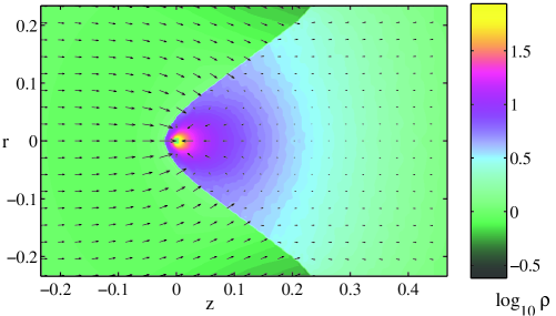
Figure 2: A hydrodynamic simulations of the BHL accretion to a non-magnetized star for Mach number ${\cal M}=3$. The central region of the flow is shown at a late time ($t=7.0t_{0}$) when the flow is stationary. The background colors represent the logarithm of the density. The arrows represent velocity vectors. Distances are measured in units of the Bondi radius $R_{\rm B}=GM/c_{s}^{2}$.

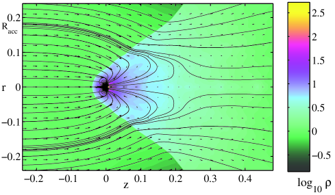
Figure 3: Matter flow around a weakly magnetized star moving through the interstellar medium with Mach number ${\cal M}=3$ at a late time $t=4.4t_{0}$. The background represents the logarithm of density and the solid lines are streamlines. The length of the arrows is proportional to the poloidal velocity

4.1 Classical Bondi-Hoyle Accretion

To test our model we performed hydrodynamic simulations of the Bondi-Hoyle accretion to a non-magnetized star for Mach number ${\cal M}=3$. Dimensionless accretion radius for this parameter $R_{\rm BH}=0.2$. The star collects matter from inside this radius. We verified that the flow is close to that described earlier in T01 where matter forms a conical shock wave.

Figure 2 shows the main features of the flow at a late time $t=7.0t_{0}$ when the flow is stationary. We calculated the accretion rate $\dot{M}$ to the numerical star and got a value $\dot{M}\approx 0.7\dot{M}_{\rm BH}$ for numerical star $R_{*}=0.0025$ were $\dot{M}_{\rm BH}$ is the Bondi-Hoyle accretion rate of equation (3) with $\alpha=1$. In our earlier calculation we got a slightly smaller value, $\dot{M}\approx 0.5\dot{M}_{\rm BH}$ for a numerical star $R_{*}=0.02$ (T01). This difference can be explained by the higher resolution of the present calculations. And this difference agrees with Ruffert’s results on the dependence of $\dot{M}$ on numerical star size for the sizes used (Ruffert 1994).

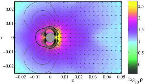
Figure 4: A central region around a weakly magnetized star moving through the interstellar medium with Mach number ${\cal M}=3$ at a late time $t=4.4t_{0}$. Zoomed-in view of the stellar magnetic field which is deformed by the flow. The thick black line surrounding the star is the magnetospheric radius $r_{m}$. The gray circle is the numerical star.

4.2 Bondi-Hoyle accretion to a star with a small magnetosphere

We performed simulations for a number of values of the magnetic moment. Initially we chose $\mu=10^{30}$Gcm³ (dimensionless moment $\mu=1.6\times 10^{-8}$), which corresponds to a star’s surface magnetic field $B=10^{12}$G. We investigated this case in detail.

Figure 3 shows the main features of the flow. Because of the magnetospheric radius $R_{\rm m}<<R_{\rm BH}$, the gravitational focusing is important and the star gathers matter from the region inside the accretion radius $R_{\rm BH}\approx 0.18$, which corresponds approximately to the theoretically derived accretion radius (Bondi-Hoyle radius) $R_{\rm BH}=0.2$. The magnetospheric radius $R_{\rm m}=0.02$ is about $10$ times smaller than the gravitational radius $R_{\rm BH}$. At the same time the average magnetospheric radius $R_{\rm m}$ is about $3$ times larger than the numerical star radius $R_{*}=0.0025$. The star’s magnetic field at distances $r>R_{\rm m}$ is significantly affected by the matter flow. An excess of matter flows from the backside of the star (return flow) and consequently the magnetic field lines are pushed towards the “front” of the star forming “ear”-like shapes. The “ears” oscillate in the $z-$direction. The conical shock wave is close to that found in the hydrodynamic case which is expected since the Mach numbers are the same.

Figure 4 shows zoomed-in view of the stellar magnetic which is deformed by the flow at a late time $t=4.4t_{0}$. The thick black line surrounding the star is the magnetospheric radius $r_{m}$ where $\rho{\bf v}^{2}={\bf B}^{2}/8\pi$.

Figure 5 shows the dependences of the density, velocity and temperature along the $z-$axis. There is a normal shock wave at $z\approx-0.04$. The density increases as the star is approached; and it is zero in the region of the star where matter is accreted. Behind the star ($z>0$) there is a strong density enhancement owing to the gravitational focusing. At $t=4.4t_{0}$ the density of matter behind the star is significantly larger than the density on the front side.

The velocity $v_{z}$ decreases sharply in the shock wave to subsonic values, but later increases again in the polar column. Behind the star the velocity is negative in the region, where accretion occurs and also increases again in the polar column to supersonic values. The plasma temperature $T$ and pressure $p$ increase strongly approaching the star along the $\pm z$ directions. This is due to the adiabatic compression of the matter.

Figure 6 shows the variation of the plasma pressure $p$, magnetic pressure $p_{\rm mag}$ and $\beta\equiv p/p_{\rm mag}$ along the $z-$axis. The dashed lines correspond to the initial distributions. One can see that the pressure $p$ gradually increases along $z-$axis, has a maximum in polar columns, and then gradually decreases. The magnetic pressure $p_{\rm mag}$ initially has a dipole shape, but it is significantly modified by the inflow of matter. Outside of the magnetosphere the matter pressure dominates.

4.3 Oscillations

We performed a number of simulation runs with different dimensionless magnetic moments ranging from $\mu=4.7\times 10^{-9}$ to $\mu=1.2\times 10^{-7}$. For relatively small magnetic moments, $\mu<2\times 10^{-8}$, we observed oscillations of the magnetic field configuration as shown in Figure 7 for our main case where $\mu=1.6\times 10^{-8}$. These oscillations are connected with the balance between back flow of the accreting matter and the tension in the distorted stellar magnetic field. Figure 7 illustrates time evolution of magnetic field lines. The field oscillations are accompanied by strong oscillations in the accretion rate to the star as shown in the top panel of Figure 8 for our main case where $\mu=1.6\times 10^{-8}$. For larger values of $\mu$ the oscillations are much weaker as shown in the bottom panel of Figure 8.

A Fourier analysis of the accretion rate oscillations for our main case gives the quasi-period of these oscillations $\Delta T\approx 0.2t_{0}=0.16R_{\rm B}/v_{\infty}=0.72R_{\rm BH}/v_{\infty}$.

Note that in hydrodynamic simulations Ruffert (1994b, 1996) observed a “flip-flop” instability of the accretion flow in 2D simulations and mass accretion rate fluctuation for smaller accretors in 3D simulations. In our simulations we see instability of the flow in case of weak or moderate magnetic field. This instability disappears as the magnetic field increases. Further, this instability is absent in our purely hydrodynamic simulation with the same parameters.

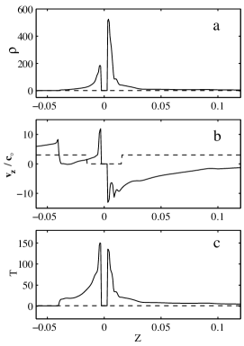
Figure 5: Panel (a) shows the density, panel (b) the axial velocity and panel (c) the temperature variation along the $z-$axis for our main case at $t=4.4t_{0}$. The dashed lines give the initial distributions.

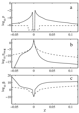
Figure 6: Panel (a) shows the matter pressure $p$, panel (b) the magnetic pressure $p_{\rm mag}$, and panel (c) $\beta=p/p_{\rm mag}$ variation along the $z-$axis for our main case at $t=4.4T_{0}$. The dashed lines give the initial distributions.

4.4 Accretion rate

For our main case the mass accretion rate is approximately $\dot{M}\approx 0.45\dot{M}_{BH}$. This value is smaller than mass accretion rate in the hydrodynamic case with the same parameters $\dot{M}\approx 0.7\dot{M}_{BH}$. Hence even a small stellar magnetic field acts to reduce the mass accretion rate. This is in agreement with the conclusions of our earlier work (T99, T03).

Figure 9 shows the observed dependence of the accretion rate on the star’s magnetic moment. It is approximately $\dot{M}\sim\mu^{-0.4}$. Note however that as $\mu$ increases, the magnetospheric radius $R_{\rm m}$ can approach the accretion radius $R_{\rm BH}$ and this can suppress the accretion.

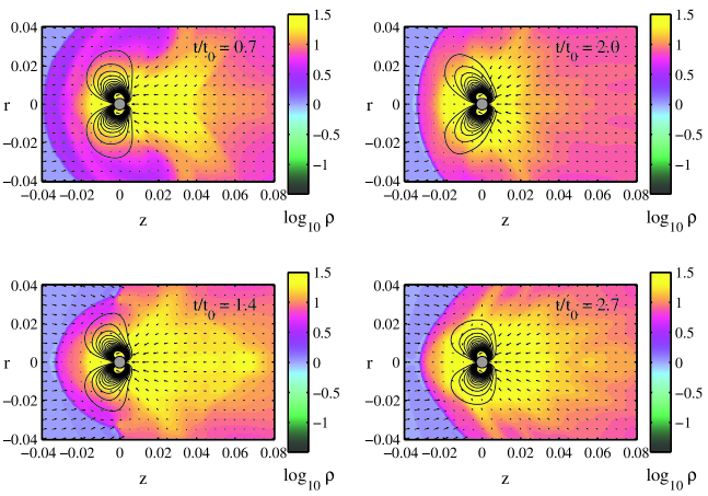
Figure 7: Matter flow around a weakly magnetized star moving with Mach number ${\cal M}=3$ at the times indicated on the plots. The background color represents the logarithm of density and the length of the arrows is proportional to the poloidal velocity.The solid lines are magnetic field lines. Distances are measured in units of the Bondi radius.

5 Astrophysical parameters

Let us consider an isolated old neutron star (IONS) moving through the interstellar medium. The star is magnetized and has a mass $M=1.4~{}M_{\odot}$. The density of the interstellar matter is assumed to be $\rho_{\infty}=1.7\times 10^{-24}$  g$/$cm³ ($n_{\infty}=1/$ cm³). The sound speed in the ISM is assumed to be $c_{s}=12$km/s so that at a Mach number ${\cal M}=3$ the star moves with a velocity $v=36$ km/s which corresponds to a relatively slow moving neutron star (Arzoumanian, Chernoff, & Cordes 2002).

The Bondi-Hoyle radius is $R_{\rm BH}=GM_{*}/v^{2}\approx 1.3\times 10^{13}{\rm cm}.$ The Bondi-Hoyle accretion rate is the $\dot{M}_{\rm BH}\approx 5\times 10^{-17}M_{\odot}$/yr for a non-magnetized star. This gives an accretion energy release rate of $L_{\rm acc}=GM\dot{M}/R_{*}\approx 6\times 10^{29}$erg/s for $R_{*}=10^{6}$cm and a non-rotating star. Both $\dot{M}$ and $L_{\rm acc}$ are reduced for magnetized star as as shown in Figure 10. With $\beta=8\pi p_{\infty}/B_{0}^{2}$ and $p_{\infty}=\rho_{ISM}c_{s}^{2}/\gamma$, we obtain the magnetic field at the surface of the numerical star $B_{0}=(8\pi/{\gamma}{\beta})^{1/2}\rho^{1/2}c_{s}\approx 0.006$G.

Recall that the size of the numerical star is $R_{*}=0.0025R_{\rm B}\approx 3\times 10^{11}{\rm cm}$ in all simulations. Thus the magnetic moment of the numerical star is $\mu=B_{0}r_{*}^{3}/2\approx 10^{30}$ Gcm³. Note that this is of the order of the magnetic moment of typical spin powered radio pulsars which have a surface field $B_{\rm NS}\approx 10^{12}$ G and radius of the order of $10^{6}$ cm. Thus we can suggest that an actual neutron star exists inside of our numerical star.

We can estimate the radius of the magnetosphere using equation (5) as $R_{\rm m}\approx 6.2\times 10^{11}{\rm cm}$. Thus $R_{\rm m}<<R_{\rm BH}$.

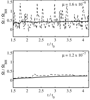
Figure 8: The top panel shows the Dependence of mass accretion rate $\dot{M}$ on time for our main case with $\mu=1.6\times 10^{-8}$ and the bottom panel a case with a stronger magnetic field, $\mu=1.2\times 10^{-7}$ The dashed lines give the mass accretion rate normalized in Bondi-Hoyle rate, while the solid lines give the integrated mass flux. Time is measured in the crossing time units, $\Delta z/v_{\infty}$.

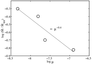
Figure 9: Dependence of the mass accretion rate $\dot{M}$ on magnetic moment $\mu$. The straight line is a least-squares straight line fit to the points.

6 Conclusions

We carried out axisymmetric MHD simulations of Bondi-Hoyle accretion onto a fast moving neutron star (${\cal M}=3$) with an aligned dipole magnetic field for cases where the Bondi-Hoyle accretion radius $R_{\rm BH}$ is much larger than the star’s magnetospheric radius $R_{\rm m}$. From this we conclude that:

1.  Interstellar matter is captured by the star if it has an impact parameter less than the accretion radius $R_{\rm BH}$. It then falls onto the star mainly onto the magnetic poles of the star. More matter falls downstream of the star. The accretion rate to the star is smaller than that to a non-magnetized star.

2.  In case of a strong stellar magnetic field ($R_{\rm m}>R_{\rm BH}$) the field is stretched in the direction of the dominant flow which towards the front side of the star.

In the case of a weak magnetic field ($R_{\rm m}<R_{\rm BH}$), the star’s field oscillates in the front/back direction. These oscillations are accompanied by strong oscillations of the mass accretion rate. The time scales of the oscillations is $\sim 0.7R_{\rm BH}/v_{\infty}$.

3.  The accretion rate decreases with increasing magnetic moment approximately as $\dot{M}\sim\mu^{-0.4}$.

4.  Old slowly rotating neutron stars with no radio emission may be visible in the X-ray band due to accretion of interstellar matter. For a neutron star moving through the interstellar medium with Mach number of $3$ we estimate the accretion luminosity as $\lesssim 10^{30}$erg s^-1. In general, the star’s velocity, magnetic moment, and angular velocity vectors may all be in different directions so that the accretion luminosity will be modulated at the star’s rotation rate.

References

- [1] Arzoumanian, Z., Chernoff, D.F., & Cordes, J.M. 2002, ApJ, 568, 289
- [2] Bisnovatyi-Kogan, G. S., Kazhdan, Y. M., Klypin, A. A., Lutskii, A. E., and Shakura, N. I.: 1979, Soviet Astronomy 23, 201
- [3] Bisnovatyi-Kogan, G. S., & Pogorelov, N. V. 1997, Astron. Astrophys. Trans., 12, 263
- [4] Bondi, H. 1952, MNRAS, 112, 195.
- [5] Bondi, H. and Hoyle, F.: 1944, MNRAS, 104, 273
- [6] Bonnell, I. A., Bate, M. R., Clarke, C. J., and Pringle, J. E.: 2001, MNRAS 323, 785
- [7] Edgar, R.G. 2004, New Astron. Rev., 48, 843
- [8] Edgar, R. and Clarke, C.: 2004, MNRAS 349, 678
- [9] Hoyle, F. and Lyttleton, R. A.: 1939, Proc. Cam. Phil. Soc. 35, 405
- [10] Lipunov, V.M. 1992, Astrophysics of Neutron Stars, (Berlin: Springer Verlag)
- [11] Petterson, J. A.: 1978, ApJ 224, 625
- [12] Pogorelov, N.V., Ohsugi, Y., & Matsuda, T. 2000, MNRAS, 313, 198
- [13] Romanova, M.M., Toropina, O.D.,Toropin, Yu.M.,& Lovelace, R.V.E., 2003, ApJ, 588, 400
- [14] Ruffert, M.: 1994a, ApJ 427, 342
- [15] Ruffert, M.: 1994b, A&AS 106, 505
- [16] Ruffert, M. and Arnett, D.: 1994, ApJ 427, 351
- [17] Ruffert, M.: 1996, A&A 311, 817
- [18] Taam, R. E. and Sandquist, E. L.: 2000, ARA&A 38, 113
- [19] Toropin, Yu.M., Toropina, O.D., Savelyev, V.V., Romanova, M.M., Chechetkin, V.M., & Lovelace, R.V.E. 1999, ApJ, 517, 906
- [20] Toropina, O.D., Romanova, M.M., Yu.M. Toropin , Yu.M.,& Lovelace, R.V.E. 2001, ApJ, 561, 964
- [21] Toropina, O.D., Romanova, M.M., Yu.M. Toropin , Yu.M.,& Lovelace, R.V.E. 2003, ApJ, 593, 472
- [22] Toropina, O.D., Romanova, M.M., & Lovelace, R.V.E. 2006, MNRAS, Volume 371, 569
- [23] Zhukov, V.T., Zabrodin, A.V., & Feodoritova, O.B. 1993, Comp. Maths. Math. Phys., 33, No. 8, 1099