Photonic band structures of periodic arrays of pores in a metallic host: tight-binding beyond the quasistatic approximation

Abstract

We have calculated the photonic band structures of metallic inverse opals and of periodic linear chains of spherical pores in a metallic host, below a plasma frequency $\omega_{\text{p}}$. In both cases, we use a tight-binding approximation, assuming a Drude dielectric function for the metallic component, but without making the quasistatic approximation. The tight-binding modes are linear combinations of the single-cavity transverse magnetic (TM) modes. For the inverse-opal structures, the lowest modes are analogous to those constructed from the three degenerate atomic $p$-states in fcc crystals. For the linear chains, in the limit of small spheres compared to a wavelength, the results are the “inverse” of the dispersion relation for metal spheres in an insulating host, as calculated by Brongersma et al. [Phys. Rev. B 62, R16356 (2000)]. Because the electromagnetic fields of these modes decay exponentially in the metal, there are no radiative losses, in contrast to the case of arrays of metallic spheres in air. We suggest that this tight-binding approach to photonic band structures of such metallic inverse materials may be a useful approach for studying photonic crystals containing metallic components, even beyond the quasistatic approximation.

I Introduction

The photonic band structures of composite materials have been studied extensively. Such band structures are defined by the relation between frequency $\omega$ and Bloch vector $\mathbf{k}$ in media in which the dielectric constant is a periodic function of position. A major reason for such interest is the possibility of producing photonic band gaps, i.e., frequency regions, extending through all $\mathbf{k}$-space, where electromagnetic waves cannot propagate through the medium. Such media have many potentially valuable applications, including possible use as filters and in films with rejection-wavelength tuning.xia In systems with a complete photonic band gap, the spontaneous emission of atoms with level splitting within the gap can be strongly suppressed.john

Since light cannot travel through the photonic band gap materials (Bragg diffracted backwards), one of their applications can be a complete control over wasteful spontaneous emission in unwanted directions when a device, such as a laser, is embedded inside a 3D photonic crystal.yablonovitch 2D photonic crystals can be used as optical microcavities, microresonators,scherer waveguides,mekis lasers, painter or fibersbenabid while 1D photonic crystals can be used as Bragg gratings or optical switches.cao

The photonic band structure of a range of materials has been studied using a plane wave expansion method. Typically, the method converges easily when the dielectric function is everywhere real, but more slowly, or not at all, when the dielectric function has a negative real part, as occurs when one component is metallic. For example, McGurn et al.mcgurn used this method to calculate the photonic band structure of a square lattice of metal cylinders in two dimensions (2D) and of an fcc lattice of metal spheres embedded in vacuum in 3D. They found that that method converged well when the filling fraction $f$ (i.e., volume fraction of metal spheres or cylinders) satisfied $f\leq 0.1\%$.

Kuzmiak et al.kuzmiak1 used the same method to calculate the photonic band structures for 2D metal cylinders in a square or triangular lattice in vacuum. For low $f$ and $\omega>\omega_{\text{p}}$, the calculated photonic band structures are just slightly perturbed versions of the dispersion curves for electromagnetic waves in vacuum. However, for $\omega<\omega_{\text{p}}$ and $\mathbf{H}$-polarized waves (magnetic field $\mathbf{H}$ parallel to the cylinders), they obtained many nearly flat bands for $\omega<\omega_{\text{p}}$; these bands were found to converge very slowly with increasing numbers of plane waves. They later extended this work to systems with dissipation.kuzmiak2 To describe dispersive and absorptive materials, they used a complex, position-dependent form of dielectric function. They also introduced a standard linearization technique to solve the resulting nonlinear eigenvalue problem.

Zabel et al.zabel extended the plane wave method to treat periodic composites with anisotropic dielectric functions. In particular, they studied the photonic band structures of a periodic array of anisotropic dielectric spheres embedded in air. They found that the anisotropy split degenerate bands, and narrowed or even closed the band gaps. Much further work on anisotropic photonic materials has been carried out since this paper (see, e.g., Ref. john ).

A different type of periodic metal-insulator composite is a periodic arrangement of metallic spheres in an insulating host. Brongersma et al.brongersma studied the dispersion relation for coupled plasmon modes in such a linear chain of equally spaced metal nanoparticles, using a near-field electromagnetic (EM) interaction between the particles in the dipole limit. They also studied the transport of EM energy around the corners and through tee junctions of the nanoparticle chain-array.

Park and Stroudpark also studied the surface-plasmon dispersion relations for a chain of metallic nanoparticles in an isotropic medium. They used a generalized tight-binding calculations, including all multipoles. This approach is more exact than the previous point-dipole calculation,brongersma in a quasistatic limit, but still leaves out non-quasistatic effects associated with radiative damping (i.e., effects associated with the non-vanishing of $\mathbf{\nabla}\times\mathbf{E}$, where $\mathbf{E}$ is the electric field. They calculated the lowest bands as well as many higher bands and compared their results with those in Ref. brongersma .

Weber and Fordweber have shown that all calculations within the quasistatic approximation omit important interactions between transverse plasmon waves and free photon modes, even if the interparticle separation is small compared to the wavelength of light. Thus, most quasistatic calculations need to have certain corrections included at particular values of the wave vector.

Recently, Gaillot et al.gaillot have studied the photonic band structures of another type of structure, a so-called inverse opal structure. This structure is an fcc lattice of void spheres in a host of another material. Such a structure can be prepared, e.g., starting from an opal structure made of spheres of a convenient substance, infiltrating it with another material, then dissolving away the spheres. In the work of Ref. gaillot , the photonic band structure of Si inverse opal was calculated as a function of the infiltrated volume fraction $f$ of air voids using three-dimensional finite difference time domain (3D FDTD) method. It was found that for certain values of $f$, a complete band gap opens up between the eighth and ninth bands.

In the present work, first we study the photonic band structure of an inverse opal structure, such as that investigated in Ref. gaillot , but instead of dielectric materials such as Si, we consider metals as the infiltrated materials. Thus, the material we study is also the inverse of the fcc array of metal spheres studied by McGurn et al.mcgurn Such metallic inverse opal structures have recently become of great interest, because it has been found that Pb inverse opals exhibit superconductivity.aliev These workers have studied the response of these materials to an applied magnetic field, and have found a highly non-monotonic fractional flux penetration into the Pb spheres as a function of the applied field.

As a second example, we study the photonic band structure of a linear chain of nanopores in a metallic medium. This is an inverse structure of a linear chain of metallic nanospheres, of which the dispersion relation is given in Ref. brongersma . As anticipated, we get a kind of “inverse image” of the dispersion relation found by Ref. brongersma in our system.

For both types of structures, our primary method for studying the photonic band structures below the plasma frequency $\omega_{\text{p}}$ is a tight-binding approximation which is valid even in the non-quasistatic regime. Because the analogs of the tight-binding atomic states decay exponentially in the metallic host medium, the resulting tight-binding waves do not lose energy radiatively, as do the corresponding waves along one-dimensional chains of metallic nanoparticles in air. Furthermore, because the modes are expanded in “atomic” states rather than plane waves, there is no convergence problem as there can be in the plane wave case.

The remainder of this paper is organized as follows. In Section II, we first present the formalism for calculating the transverse magnetic (TM) and transverse electric (TE) modes of a single spherical cavity in a metallic host. We then describe the method for calculating the photonic band structures of metallic inverse opals and of linear chains of nanopores in a metallic host, using a simple tight-binding approach for $\omega<\omega_{\text{p}}$. In Section III, we give the numerical results for the TM and TE modes of a single cavity and those of the tight-binding method for the metal inverse opals and the linear chain of nanopores. Section IV presents a summary and discussion.

II Formalism

In this section, we present a summary of the equations determining the band structure of a photonic crystal containing a metallic component with Drude dielectric function $\epsilon(\omega)=1-\omega_{\text{p}}^{2}/\omega^{2}$ and an insulating component of dielectric constant unity. The insulating component is assumed to be present in the form of identical spherical cavities of radius $R$. We first write down the equations for the TM and TE modes of a spherical cavity in a Drude metal. Then, we present a tight-binding method for $\omega<\omega_{\text{p}}$.

II.1 Spherical Cavity

As a preliminary to calculating the photonic band structure, we first discuss the modes of a single spherical cavity in a Drude metal host. We begin with the TM modes of the cavity, then the TE modes.

II.1.1 TM Modes

It is convenient to describe the modes of the embedded cavity in terms of the $\mathbf{B}$ field. To that end, we combine the two homogeneous Maxwell equations

$$\mathbf{\nabla}\times\mathbf{E} = \frac{i\omega}{c}\mathbf{B},$$ (1)

$$\mathbf{\nabla}\times\mathbf{B} = -\frac{i\omega}{c}\epsilon\mathbf{E},$$ (2)

to obtain a single equation for $\mathbf{B}$:

$$\mathbf{\nabla}\times\left[\left\{\frac{1}{1-\frac{\omega_{\text{p}}^{2}}{\omega^{2}}}\theta(\mathbf{x})+1-\theta(\mathbf{x})\right\}\mathbf{\nabla}\times\mathbf{B}\right]=\frac{\omega^{2}}{c^{2}}\mathbf{B}.$$ (3)

Here, we have expressed the position- and frequency-dependent dielectric function $\epsilon(\mathbf{x},\omega)$ as $1/\epsilon(\mathbf{x},\omega)=\theta(\mathbf{x})/(1-\omega_{\text{p}}^{2}/\omega^{2})+1-\theta(\mathbf{x})$, where the step function $\theta(\mathbf{x})=1$ inside the metallic region and $\theta(\mathbf{x})=0$ elsewhere. Multiplying this equation by $\omega^{2}-\omega_{\text{p}}^{2}$ and simplifying, we obtain

$$[\omega^{2}-\omega_{\text{p}}^{2}(1-\theta(\mathbf{x}))]\mathbf{\nabla}\times(\mathbf{\nabla}\times\mathbf{B})=\frac{\omega^{2}}{c^{2}}(\omega^{2}-\omega_{\text{p}}^{2})\mathbf{B}.$$ (4)

Thus, inside the spherical void, we have

$$\mathbf{\nabla}\times(\mathbf{\nabla}\times\mathbf{B})=\frac{\omega^{2}}{c^{2}}\mathbf{B},$$ (5)

while inside the metal,

$$\mathbf{\nabla}\times(\mathbf{\nabla}\times\mathbf{B})=\frac{\omega^{2}-\omega_{\text{p}}^{2}}{c^{2}}\mathbf{B}.$$ (6)

For a spherical void within a metallic host, it is convenient to solve these equations in spherical coordinates. It is readily found that, for the TM modes, the non-vanishing components of the solutions for $\mathbf{B}$ and $\mathbf{E}$ for Eq. (5) and Eq. (2) arejackson

$$B_{\phi,\text{in}}(r,\theta)=\frac{u_{\ell}(r)}{r}P_{\ell}^{1}(\cos\theta),$$

$$E_{r,\text{in}}=-\frac{ic}{\omega r}\ell(\ell+1)\frac{u_{\ell}(r)}{r}P_{\ell}(\cos\theta),$$

$$E_{\theta,\text{in}}=-\frac{ic}{\omega r}\frac{\partial u_{\ell}(r)}{\partial r}P_{\ell}^{1}(\cos\theta),$$

$$u_{\ell}(r)=r[A_{\ell}j_{\ell}(kr)+B_{\ell}n_{\ell}(kr)],$$ (7)

where $k=\omega/c$, $j_{\ell}$ and $n_{\ell}$ are spherical Bessel functions, and the subscripts $\phi$, $r$, and $\theta$ denote components of the corresponding fields in spherical coordinates.

Likewise, the solutions of Eqs. (6) and (2) within the metal will be

$$B_{\phi,\text{out}}(r,\theta)=\frac{v_{\ell}(r)}{r}P_{\ell}^{1}(\cos\theta),$$

$$E_{r,\text{out}}=-\frac{ic}{\omega r\left(1-\frac{\omega_{\text{p}}^{2}}{\omega^{2}}\right)}\ell(\ell+1)\frac{v_{\ell}(r)}{r}P_{\ell}(\cos\theta),$$

$$E_{\theta,\text{out}}=-\frac{ic}{\omega r\left(1-\frac{\omega_{\text{p}}^{2}}{\omega^{2}}\right)}\frac{\partial v_{\ell}(r)}{\partial r}P_{\ell}^{1}(\cos\theta),$$

$$v_{\ell}(r)=r[C_{\ell}j_{\ell}(k^{\prime}r)+D_{\ell}n_{\ell}(k^{\prime}r)],$$ (8)

where $k^{\prime}=\sqrt{\omega^{2}-\omega_{\text{p}}^{2}}/c$.

The requirements that the normal displacement $D$ and tangential $E$ should be continuous at $R$ gives the two conditions

$$u_{\ell}(R)=v_{\ell}(R)$$ (9)

and

$$\left.\frac{\partial u_{\ell}(r)}{\partial r}\right|_{r=R}=\frac{1}{\left(1-\frac{\omega_{\text{p}}^{2}}{\omega^{2}}\right)}\left.\frac{\partial v_{\ell}(r)}{\partial r}\right|_{r=R}=\frac{k^{2}}{k^{\prime 2}}\left.\frac{\partial v_{\ell}(r)}{\partial r}\right|_{r=R},$$ (10)

where $R$ is the radius of the spherical cavity. Since the fields at the center of the void sphere must be finite, we also have

$$u_{\ell}(r)=rj_{\ell}(kr),$$ (11)

where we have normalized the solution so that the coefficient $A_{\ell}=1$. From Eq. (9) we have

$$j_{\ell}(kR)=C_{\ell}j_{\ell}(k^{\prime}R)+D_{\ell}n_{\ell}(k^{\prime}R),$$ (12)

whereas, from Eq. (10), we get

$$k^{\prime 2}\left[j_{\ell}(kR)+kRj_{\ell}^{\prime}(kR)\right]$$ (13)

$$= k^{2}\left[C_{\ell}j_{\ell}(k^{\prime}R)+D_{\ell}n_{\ell}(k^{\prime}R)+k^{\prime}R\left\{C_{\ell}j_{\ell}^{\prime}(k^{\prime}R)\right.\right.$$

$$+\left.\left.D_{\ell}n_{\ell}^{\prime}(k^{\prime}R)\right\}\right].$$

The coefficients $C_{\ell}$ and $D_{\ell}$ can then be determined from these boundary conditions.

The results for $\omega<\omega_{\text{p}}$, can be obtained by making the substitution $k^{\prime}\rightarrow ik^{\prime}$, with $k^{\prime}$ real. In this case, the radial component of Eq. (6) takes the form

$$\frac{\partial^{2}u_{\ell}}{\partial r^{2}}-\left[\frac{1}{c^{2}}(\omega_{\text{p}}^{2}-\omega^{2})+\frac{\ell(\ell+1)}{r^{2}}\right]u_{\ell}=0,$$ (14)

which is the modified Bessel equation. The solutions of Eq. (14) are the modified spherical Bessel functions $i_{\ell}$ and $k_{\ell}$ (note that this $k_{\ell}$ is different from the wave vectors $k$ and $k^{\prime}$). In this case, Eq. (8) becomes

$$v_{\ell}(r)=r[C_{\ell}i_{\ell}(k^{\prime}r)+D_{\ell}k_{\ell}(k^{\prime}r)],$$ (15)

where $k^{\prime}=\sqrt{\omega_{\text{p}}^{2}-\omega^{2}}/c$. In addition, Eqs. (10), (12), and (13) are transformed, respectively, into

$$\left.\frac{\partial u_{\ell}(r)}{\partial r}\right|_{r=R}=-\frac{k^{2}}{k^{\prime 2}}\left.\frac{\partial v_{\ell}(r)}{\partial r}\right|_{r=R},$$ (16)

$$j_{\ell}(kR)=C_{\ell}i_{\ell}(k^{\prime}R)+D_{\ell}k_{\ell}(k^{\prime}R),$$ (17)

and

$$k^{\prime 2}\left[j_{\ell}(kR)+kRj_{\ell}^{\prime}(kR)\right]=-k^{2}\left[C_{\ell}i_{\ell}(k^{\prime}R)\right.$$

$$\left.+D_{\ell}k_{\ell}(k^{\prime}R)+k^{\prime}R\left\{C_{\ell}i_{\ell}^{\prime}(k^{\prime}R)+D_{\ell}k_{\ell}^{\prime}(k^{\prime}R)\right\}\right].$$ (18)

It is of interest to consider the specific case of a spherical cavity in an infinite medium. In this case, $C_{\ell}=0$ because $i_{\ell}(x)$ diverges at large $x$. As a result, Eqs. (15), (17), and (18) become, respectively,

$$v_{\ell}(r)=rD_{\ell}k_{\ell}(k^{\prime}r),$$ (19)

$$j_{\ell}(kR)=D_{\ell}k_{\ell}(k^{\prime}R),$$ (20)

and

$$k^{\prime 2}\left[j_{\ell}(kR)+kRj_{\ell}^{\prime}(kR)\right]=-k^{2}D_{\ell}\left[k_{\ell}(k^{\prime}R)\right.$$

$$\left.+k^{\prime}Rk_{\ell}^{\prime}(k^{\prime}R)\right].$$ (21)

From Eq. (20) we have $D_{\ell}=j_{\ell}(kR)/k_{\ell}(k^{\prime}R)$, and hence Eq. (21) becomes

$$k^{\prime 2}\left[j_{\ell}(kR)+kRj_{\ell}^{\prime}(kR)\right]=-k^{2}\frac{j_{\ell}(kR)}{k_{\ell}(k^{\prime}R)}\left[k_{\ell}(k^{\prime}R)\right.$$

$$\left.+k^{\prime}Rk_{\ell}^{\prime}(k^{\prime}R)\right].$$ (22)

We can readily obtain the asymptotic forms of the solutions when $kR\ll 1$ and $k^{\prime}R\ll 1$. In this case $j_{\ell}(kR)$ and $k_{\ell}(k^{\prime}R)$ have the asymptotic forms $j_{\ell}(kR)\approx(kR)^{\ell}/(2\ell+1)!!$ and $k_{\ell}(k^{\prime}R)\approx\sqrt{\pi}\Gamma(\ell+1/2)2^{\ell-1}/(k^{\prime}R)^{\ell+1}$. In this limit, Eq. (22), after some algebra, reduces to simply

$$k^{\prime 2}(\ell+1)=k^{2}\ell.$$ (23)

Since $k^{\prime}=\sqrt{\omega_{\text{p}}^{2}-\omega^{2}}/c$, Eq. (23) is equivalent to

$$\omega^{2}=\frac{\ell+1}{2\ell+1}\omega_{\text{p}}^{2}.$$ (24)

The largest value, $\omega=\sqrt{2/3}\omega_{\text{p}}$, occurs at $\ell=1$ and the limiting value for large $\ell$ is $\omega=\omega_{\text{p}}/\sqrt{2}$.

II.1.2 TE Modes

For the TE mode, inside the spherical void, we have

$$\mathbf{\nabla}\times(\mathbf{\nabla}\times\mathbf{E})=\frac{\omega^{2}}{c^{2}}\mathbf{E},$$ (25)

whereas inside the metal, we have

$$\mathbf{\nabla}\times(\mathbf{\nabla}\times\mathbf{E})=\frac{\omega^{2}-\omega_{\text{p}}^{2}}{c^{2}}\mathbf{E}.$$ (26)

We now use these equations to calculate $E_{\phi}$, $B_{r}$, and $B_{\theta}$. From Eq. (25) we get

$$E_{\phi,\text{in}}(r,\theta)=\frac{u_{\ell}(r)}{r}P_{\ell}^{1}(\cos\theta),$$

$$B_{r,\text{in}}=\frac{ic}{\omega r}\ell(\ell+1)\frac{u_{\ell}(r)}{r}P_{\ell}(\cos\theta),$$

$$B_{\theta,\text{in}}=\frac{ic}{\omega r}\frac{\partial u_{\ell}(r)}{\partial r}P_{\ell}^{1}(\cos\theta),$$

$$u_{\ell}(r)=r[A_{\ell}j_{\ell}(kr)+B_{\ell}n_{\ell}(kr)],$$ (27)

where $k=\omega/c$. The solutions of Eq. (26) are

$$E_{\phi,\text{out}}(r,\theta)=\frac{v_{\ell}(r)}{r}P_{\ell}^{1}(\cos\theta),$$

$$B_{r,\text{out}}=\frac{ic}{\omega r}\ell(\ell+1)\frac{v_{\ell}(r)}{r}P_{\ell}(\cos\theta),$$

$$B_{\theta,\text{out}}=\frac{ic}{\omega r}\frac{\partial v_{\ell}(r)}{\partial r}P_{\ell}^{1}(\cos\theta),$$

$$v_{\ell}(r)=r[C_{\ell}j_{\ell}(k^{\prime}r)+D_{\ell}n_{\ell}(k^{\prime}r)],$$ (28)

where $k^{\prime}=\sqrt{\omega^{2}-\omega_{\text{p}}^{2}}/c$.

Since normal $B$ and tangential $H$ should be continuous on the boundaries, we obtain the conditions

$$u_{\ell}(R)=v_{\ell}(R),$$ (29)

as in the TM case, and

$$\left.\frac{\partial u_{\ell}(r)}{\partial r}\right|_{r=R}=\left.\frac{\partial v_{\ell}(r)}{\partial r}\right|_{r=R}.$$ (30)

Since the fields must be finite at the center of the void sphere, we can choose

$$u_{\ell}(r)=rj_{\ell}(kr),$$ (31)

we also take the coefficient $A_{\ell}=1$. From Eq. (29) we have

$$j_{\ell}(kR)=C_{\ell}j_{\ell}(k^{\prime}R)+D_{\ell}n_{\ell}(k^{\prime}R),$$ (32)

while, from Eq. (30), we get

$$j_{\ell}(kR)+kRj_{\ell}^{\prime}(kR)$$ (33)

$$= C_{\ell}j_{\ell}(k^{\prime}R)+D_{\ell}n_{\ell}(k^{\prime}R)+k^{\prime}R\left[C_{\ell}j_{\ell}^{\prime}(k^{\prime}R)\right.$$

$$\left.+D_{\ell}n_{\ell}^{\prime}(k^{\prime}R)\right].$$

The corresponding equation for $\omega<\omega_{\text{p}}$, can again be obtained by the transformation $k^{\prime}\rightarrow ik^{\prime}$. The TE modes for $\omega<\omega_{\text{p}}$ using the modified spherical Bessel functions $i_{\ell}(x)$ and $k_{\ell}(x)$ satisfy Eqs. (14), (15), (30), and (17). The only changes are in Eq. (18), which becomes

$$j_{\ell}(kR)+kRj_{\ell}^{\prime}(kR)=C_{\ell}i_{\ell}(k^{\prime}R)+D_{\ell}k_{\ell}(k^{\prime}R)$$

$$+k^{\prime}R\left\{C_{\ell}i_{\ell}^{\prime}(k^{\prime}R)+D_{\ell}k_{\ell}^{\prime}(k^{\prime}R)\right\}.$$ (34)

In an infinite medium, these conditions become, from Eq. (20),

$$j_{\ell}(kR)+kRj_{\ell}^{\prime}(kR)=\frac{j_{\ell}(kR)}{k_{\ell}(k^{\prime}R)}\left[k_{\ell}(k^{\prime}R)+k^{\prime}Rk_{\ell}^{\prime}(k^{\prime}R)\right].$$ (35)

If we consider the asymptotic forms of the solutions when $kR\ll 1$ and $k^{\prime}R\ll 1$ as we did for the TM modes, Eq. (35) simplifies to

$$\ell+1=-\ell,$$ (36)

which gives $\ell=-1/2$. Since $\ell$ must be a positive integer, we see that there are no eigenvalues for TE modes in the limit $kR\ll 1$ and $k^{\prime}R\ll 1$.

II.2 Tight-Binding Approach to Modes for $\omega<\omega_{\text{p}}$

We now turn from describing the single-cavity modes to a discussion of the band structure for a periodic array of such cavities. In conventional periodic solids, the tight-binding method is very useful in treating narrow bands. In what follows, we try to suggest an analogous tight-binding approach for the lowest set of TM modes in a periodic lattice of spherical cavities in a metallic host, in the frequency range $\omega<\omega_{\text{p}}$. We apply the resulting method, first, to an fcc lattice of pores, and then to a linear chain of spherical pores in a metallic host.

Even though these are TM modes, it is convenient to describe them now in terms of their electric fields. We denote the electric field of the $\lambda$th mode by $\mathbf{E}_{\lambda}(\mathbf{x})$. This field satisfies

$$\mathbf{\nabla}\times(\mathbf{\nabla}\times\mathbf{E}_{\lambda}(\mathbf{x}))+\frac{\omega_{\text{p}}^{2}\theta(\mathbf{x})}{c^{2}}\mathbf{E}_{\lambda}(\mathbf{x})\equiv\mathcal{O}\mathbf{E}_{\lambda}(\mathbf{x})=\frac{\omega_{\lambda}^{2}}{c^{2}}\mathbf{E}_{\lambda}(\mathbf{x}),$$ (37)

where $\mathcal{O}=\mathbf{\nabla}\times(\mathbf{\nabla}\times)+(\omega_{\text{p}}^{2}/c^{2})\theta(\mathbf{x})$ is the “Hamiltonian” of this system. Since $\mathcal{O}$ is a Hermitian operator, the eigenstates corresponding to unequal eigenvalues $\omega_{\lambda}^{2}/c^{2}$ and $\omega_{\mu}^{2}/c^{2}$ are orthogonal and may be chosen to be orthonormal. (The orthogonality may also be proved directly by integration by parts.) The orthonormality relation is

$$\int\mathbf{E}_{\lambda}^{*}(\mathbf{x})\cdot\mathbf{E}_{\mu}(\mathbf{x})d\mathbf{x}=\delta_{\lambda,\mu}.$$ (38)

Since $\mathbf{E}_{\lambda}(\mathbf{x})$ is real for $\omega<\omega_{\text{p}}$, the complex conjugation is, in fact, unnecessary.

In Sec. II.1.1, our paper already gives the equations determining the electric and magnetic fields of isolated TM modes for a spherical cavity. The lowest set corresponds to $\ell=1$, and there should be three of these. For a spherical cavity, all three are degenerate, i.e., all three have the same eigenfrequencies. Even though the three modes have equal frequencies, one can always choose an orthonormal set, with electric fields $\mathbf{E}_{1}$, $\mathbf{E}_{2}$, and $\mathbf{E}_{3}$ satisfying the orthonormality relation in Eq. (38).

In order to obtain the tight-binding band structure built from these three modes, we need to calculate matrix elements of the form

$$M_{\alpha,\beta}(\mathbf{R})=\int\mathbf{E}_{\alpha}^{*}(\mathbf{x})\cdot\mathcal{O}\mathbf{E}_{\beta}(\mathbf{x}-\mathbf{R})d\mathbf{x},$$ (39)

corresponding to two single-cavity modes associated with different cavities centered at the origin and at $\mathbf{R}$. Here, $\mathcal{O}$ is the “Hamiltonian” of the system as defined implicitly in Eq. (37).

Next, we introduce normalized Bloch states associated with the three $\ell=1$ single-cavity modes. In order to do this, we first make the usual tight-binding assumption that the “atomic” states corresponding to different cavities are orthogonal:

$$\int\mathbf{E}_{\lambda}^{*}(\mathbf{x}-\mathbf{R})\cdot\mathbf{E}_{\mu}(\mathbf{x}-\mathbf{R}^{\prime})d\mathbf{x}=\delta_{\lambda,\mu}\delta_{\mathbf{R},\mathbf{R}^{\prime}}.$$ (40)

This orthogonality of states on different cavities is reasonable since the fields fall off exponentially with separation.

The orthonormal Bloch states then take the form

$$\mathbf{E}_{\mathbf{k},\lambda}(\mathbf{x})=N^{-1/2}\sum_{\mathbf{R}}e^{i\mathbf{k}\cdot\mathbf{R}}\mathbf{E}_{\lambda}(\mathbf{x}-\mathbf{R}),$$ (41)

where $\mathbf{k}$ is a Bloch vector, and the $\mathbf{R}$’s are the Bravais lattice vectors. In writing Eq. (41), we have assumed that there are $N$ identical spherical cavities, and that the Bloch states satisfy the usual periodic boundary conditions of Born-von Karman type. We also introduce the elements of the “Hamiltonian” matrix

$$M_{\lambda,\mu}(\mathbf{k})=\sum_{\mathbf{R}}e^{i\mathbf{k}\cdot\mathbf{R}}M_{\lambda,\mu}(\mathbf{R}).$$ (42)

We can then obtain the frequencies $\omega(\mathbf{k})$ by diagonalizing a $3\times 3$ matrix as follows:

$$det\left|M_{\lambda,\mu}(\mathbf{k})-\left(\frac{\omega^{2}(\mathbf{k})}{c^{2}}-\frac{\omega_{\text{at}}^{2}}{c^{2}}\right)\delta_{\lambda,\mu}\right|=0,$$ (43)

where $\omega_{\text{at}}$ is the eigenvalue of a single-cavity mode. The solutions to these equations give the three $p$-bands for a periodic lattice of cavities in a metallic host. This procedure is analogous to that used in the well-known procedure for obtaining tight-binding bands from three degenerate $p$-bands in the electronic structure of conventional solids (see, for example, Ref. ashcroft ).

We briefly comment on the connection between this approach and that used by earlier workers.brongersma ; park In this work, the authors treat wave propagation along a chain of metallic nanoparticles. They use the tight-binding approximation, as we do, but in the quasistatic approximation in which one assumes that $\mathbf{\nabla}\times\mathbf{E}=0$. This approximation is reasonable when both the particle radii and the interparticle separations are small compared to a wavelength, but is not accurate in other circumstances. Furthermore, even in the small-particle and small-separation regime, this approximation still fails to account for the radiation which occurs at certain wave numbers and frequencies. The present approach would generalize this tight-binding method to (a) three dimensions as well as one; (b) pore modes instead of small particle modes; and most importantly (c) larger pores and larger interparticle separations, via extension beyond the quasistatic approximation.

Next, we discuss the numerical evaluation of the required matrix elements, Eq. (39). The relevant electric fields are given in this paper, but in spherical coordinates. It is not difficult to convert these into Cartesian coordinates. The operator $\mathcal{O}$ is just a little trickier. We first note that $\mathcal{O}=\mathcal{O}_{\mathbf{R}}+\mathcal{O}^{\prime}$, where $\mathcal{O}_{\mathbf{R}}$ is the single-cavity operator: $\mathcal{O}_{\mathbf{R}}=\mathbf{\nabla}\times(\mathbf{\nabla}\times$) if $\mathbf{x}$ is inside the $\mathbf{R}$th cavity and $\mathcal{O}_{\mathbf{R}}=\mathbf{\nabla}\times(\mathbf{\nabla}\times)+\omega_{\text{p}}^{2}/c^{2}$ otherwise. Now we also have

$$\mathcal{O}_{\mathbf{R}}\mathbf{E}_{\beta}(\mathbf{x}-\mathbf{R}^{\prime})=\frac{\omega_{\text{at}}^{2}}{c^{2}}\mathbf{E}_{\beta}(\mathbf{x}-\mathbf{R}^{\prime}),$$ (44)

since $\mathbf{E}_{\beta}$ is an eigenstate of $\mathcal{O}_{\mathbf{R}}$ with an eigenvalue $\omega_{\text{at}}^{2}/c^{2}$.

But since we are assuming that the overlap integral between “atomic” electric field states centered on different sites vanishes, the term involving $\mathcal{O}_{\mathbf{R}}$ does not contribute to the matrix element $M_{\alpha,\beta}$, which is therefore just given by

$$M_{\alpha,\beta}(\mathbf{R})=\int\mathbf{E}_{\alpha}(\mathbf{x})\cdot\mathcal{O}^{\prime}\mathbf{E}_{\beta}(\mathbf{x}-\mathbf{R})d\mathbf{x}.$$ (45)

We can also write

$$\mathcal{O}^{\prime}=\frac{\omega_{\text{p}}^{2}}{c^{2}}\sum_{\mathbf{R}^{\prime}}\theta_{\mathbf{R}^{\prime}}(\mathbf{x}),$$ (46)

where

$$\theta_{\mathbf{R^{\prime}}}=\theta(\mathbf{x}-\mathbf{R}^{\prime}),$$ (47)

is a step function which is unity inside the cavity centered at $\mathbf{R}^{\prime}$ and is zero otherwise.

A reasonable approximation to Eq. (46) might be to include just $\mathbf{R}^{\prime}=0$. In this case, we finally will get

$$M_{\alpha,\beta}(\mathbf{R})\sim\frac{\omega_{\text{p}}^{2}}{c^{2}}\int\mathbf{E}_{\alpha}(\mathbf{x})\cdot\mathbf{E}_{\beta}(\mathbf{x}-\mathbf{R})d\mathbf{x},$$ (48)

where the integral runs just over the cavity centered at the origin. As a further approximation, we can just replace $\mathbf{E}_{\beta}(\mathbf{x}-\mathbf{R})$ by the value of this function at the origin, i.e., $\mathbf{E}_{\beta}(-\mathbf{R})$. Then this field can be taken outside the integral and we just have

$$M_{\alpha,\beta}(\mathbf{R})\sim\frac{\omega_{\text{p}}^{2}}{c^{2}}\mathbf{E}_{\beta}(-\mathbf{R})\cdot\int\mathbf{E}_{\alpha}(\mathbf{x})d\mathbf{x},$$ (49)

where once again the integral runs over the cavity centered at the origin.

Next, we attempt to calculate the relevant quantities needed to solve for this matrix element. In order to use the tight-binding approach we will need to normalize the individual eigenstates $\mathbf{E}_{\alpha}$. Therefore, we will begin by obtaining this normalization. For $\ell=1$, the $u_{\ell}(r)$’s are $r$ times spherical Bessel functions. We write this field as

$$E_{r,\text{in}}=+\frac{2C_{1}}{kr}j_{1}(kr)\cos\theta,$$ (50)

where we have used the relation $P_{1}(\cos\theta)=\cos\theta$, and introduced the normalization constant $C_{1}$, which will be determined below. Similarly,

$$E_{\theta,\text{in}}=-\frac{C_{1}}{kr}\frac{\partial[rj_{1}(kr)]}{\partial r}\sin\theta,$$ (51)

where we use $P_{1}^{1}(\cos\theta)=-\sin\theta$. For $r>R$, we have

$$E_{r,\text{out}}=+\frac{2D_{1}C_{1}}{k^{\prime}r}k_{1}(k^{\prime}r)\cos\theta$$ (52)

and

$$E_{\theta,\text{out}}=-\frac{D_{1}C_{1}}{k^{\prime}r}\frac{\partial[rk_{1}(k^{\prime}r)]}{\partial r}\sin\theta.$$ (53)

We will need the integrals of the Cartesian components of the field over the volume of the sphere centered at the origin. Let us assume we are considering the $z$ mode, i.e., the one for which $\theta$ refers to the angle from the $z$ axis. Then the symmetry of the problem shows that only the $z$ component of the electric field will have a nonzero integral. Also, we have that

$$E_{z,\text{in}}(r,\theta)=E_{r,\text{in}}\cos\theta-E_{\theta,\text{in}}\sin\theta.$$ (54)

Thus, after a little algebra, we find that the integral of this field over the volume of the cavity is

$$\int E_{z,\text{in}}(r,\theta)d\mathbf{r}=\frac{8\pi C_{1}}{3k}R^{2}j_{1}(kR).$$ (55)

Next, we work out the coefficient $D_{1}$. It is determined by the boundary conditions at $r=R$. These conditions are that $D_{r}$ and $E_{\theta}$ should be continuous at $r=R$. These two conditions determine not only the value of $D_{1}$ but also the allowed frequency. After a bit of algebra, we find that

$$D_{1}=\frac{\omega^{2}}{c^{2}kk^{\prime}}\frac{j_{1}(kR)}{k_{1}(k^{\prime}R)}=\frac{k}{k^{\prime}}\frac{j_{1}(kR)}{k_{1}(k^{\prime}R)}.$$ (56)

The allowed value of $\omega$ is given by Eq. (22).

Finally, we need the normalization constant $C_{1}$. We choose this so that the integral of the square of the electric field for a single-cavity mode should be normalized to unity. This condition may be written

$$\frac{2C_{1}^{2}}{k^{2}}\frac{4\pi}{3}\int_{0}^{R}\left[2j_{1}^{2}(kr)+\left(\frac{\partial[rj_{1}(kr)]}{\partial r}\right)^{2}\right]dr$$ (57)

$$+ \frac{2C_{1}^{2}D_{1}^{2}}{k^{\prime 2}}\frac{4\pi}{3}\int_{R}^{\infty}\left[2k_{1}^{2}(k^{\prime}r)+\left(\frac{\partial[rk_{1}(k^{\prime}r)]}{\partial r}\right)^{2}\right]dr$$

$$= 1.$$

If we write

$$\int_{0}^{kR}\left[2j_{1}^{2}(x)+\left(\frac{d[xj_{1}(x)]}{dx}\right)^{2}\right]dx=F_{1}(kR)$$ (58)

and

$$\int_{k^{\prime}R}^{\infty}\left[2k_{1}^{2}(x)+\left(\frac{d[xk_{1}(x)]}{dx}\right)^{2}\right]dx=F_{2}(k^{\prime}R),$$ (59)

then we can express the normalization condition as

$$\frac{8\pi C_{1}^{2}}{3}\left[\frac{F_{1}(kR)}{k^{3}}+D_{1}^{2}\frac{F_{2}(k^{\prime}R)}{k^{\prime 3}}\right]=1.$$ (60)

Therefore, we can now write out an explicit expression for the matrix element $M_{\alpha,\beta}(\mathbf{R})$ given in Eq. (49). For the $\alpha$th mode, the integral of $\mathbf{E}_{\alpha}$ over the volume of a cavity is a vector in the $\alpha$th direction. To evaluate Eq. (49), we need the component of the $\alpha$th mode in the $\beta$th direction at a position $\mathbf{R}$. Let us first consider the $z$th mode ($\alpha=z$). We can use Eqs. (52) and (53) to rewrite this field in Cartesian coordinates with the additional equations

$$\cos\theta = \frac{z}{r},$$

$$\sin\theta = \frac{\sqrt{x^{2}+y^{2}}}{r},$$

$$\hat{r} = \frac{x\hat{x}+y\hat{y}+z\hat{z}}{r},$$

$$\hat{\theta} = \frac{xz\hat{x}+yz\hat{y}}{r\sqrt{x^{2}+y^{2}}}-\frac{\sqrt{x^{2}+y^{2}}}{r}\hat{z}.$$ (61)

We just substitute these expressions back into Eqs. (52) and (53) to get the Cartesian components of the field for a mode parallel to the $z$ axis. For the mode parallel to the $x$ axis, we just permute the coordinates cyclically: $z\rightarrow x$, $x\rightarrow y$, and $y\rightarrow z$. Similarly, for the $y$ modes, we make the permutation $(x,y,z)\rightarrow(z,x,y)$.

Using these results, we should be able to compute all the elements in the tight-binding matrix and hence obtain the band structure for the photonic $p$-bands in the tight-binding approximation, in either one or three dimensions.

III Numerical Results

For the inverse opals we arbitrarily assume a lattice constant $d=500\sqrt{2}\>\text{nm}$, and a void sphere radius $R=150\>\text{nm}$ as in Fig. 1(a). This choice is the same as that of Ref. aliev , where the Pb inverse opal has this lattice constant. Since the volume of the primitive unit cell is $v_{c}=d^{3}/4$, this corresponds to a void volume fraction $f=0.160$. For the linear chain of nanopores (see below) this $d$ is the separation between two nanopores and $R$ is the radius of a nanopore as in Fig. 1(b).

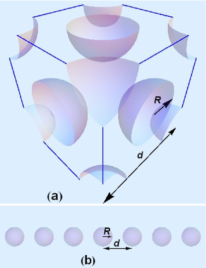
Figure 1: (Color online) Schematic diagram for (a) an inverse opal structure with a lattice constant $d$ and a void sphere radius $R$; (b) a linear chain of nanopores with a pore separation $d$ and a nanopore radius $R$.

Our band structures for the inverse opals are expressed in terms of the standard notation for $\mathbf{k}$ values at symmetry points in the Brillouin zone. These are $\Gamma=(0,0,0)$, $X=(2\pi/d)(0,0,1)$, $U=(2\pi/d)(1/4,1/4,1)$, $L=(2\pi/d)(1/2,1/2,1/2)$, $W=(2\pi/d)(1/2,0,1)$, and $K=(2\pi/d)(3/4,0,3/4)$.

The metallic dielectric functions we assume for the inverse opals and linear chain of nanopores are of the usual Drude form,

$$\epsilon(\omega)=1-\frac{\omega_{\text{p}}^{2}}{\omega^{2}},$$ (62)

where $\omega_{\text{p}}$ is the plasma frequency of the conduction electrons. $\epsilon(\omega)<0$ when $\omega<\omega_{\text{p}}$, while $\epsilon(\omega)>0$ when $\omega>\omega_{\text{p}}$. Our calculations are thus carried out assuming that the Drude relaxation time $\tau\rightarrow\infty$. For a metal in its normal state, $\omega_{\text{p}}^{2}=4\pi ne^{2}/m$, where $n$ is the conduction electron density and $m$ is the electron mass. Note that with this choice of dielectric function, the entire band structure can be expressed in scaled form. That is, the scaled frequency $\omega d/c$ is a function only of the scaled wave vector $kd$, and the band structures are parameterized by the two constants $\omega_{\text{p}}d/c$ and $f$ for the case of inverse opals.

Since we are considering void spheres in inverse opals and linear chains of nanopores, it is of interest to consider electromagnetic wave modes in a single cavity, which could be considered a single “atom” of the void lattice. We show only results for $\omega<\omega_{\text{p}}$, since these are the results most relevant to possible narrow-band photonic states in the inverse opal structure. Our results for $\omega<\omega_{\text{p}}$ for an isolated spherical cavity in an infinite medium, and when $kR\ll 1$ and $k^{\prime}R\ll 1$ are given in Table 1. These two inequalities are reasonable for our inverse opal system parameters $d=500\sqrt{2}\>\text{nm}$, $R=150\>\text{nm}$, and $\omega_{\text{p}}d/c=1$, because

$$kR = \frac{\omega}{c}R<\frac{\omega_{\text{p}}}{c}R=\frac{\omega_{\text{p}}d}{c}\frac{R}{d}=\frac{3}{10\sqrt{2}}=0.2121,$$

$$k^{\prime}R = \frac{\sqrt{\omega_{\text{p}}^{2}-\omega^{2}}}{c}R=\sqrt{\left(\frac{\omega_{\text{p}}R}{c}\right)^{2}-\left(\frac{\omega R}{c}\right)^{2}}$$ (63)

$$= \sqrt{\left(\frac{\omega_{\text{p}}d}{c}\frac{R}{d}\right)^{2}-(kR)^{2}}=\sqrt{\left(\frac{3}{10\sqrt{2}}\right)^{2}-(kR)^{2}}$$

$$= \sqrt{0.045-(kR)^{2}}<\sqrt{0.045}=0.2121.$$

The (modified) spherical Bessel functions in Eq. (22) are extremely close to the $\omega$ axis for $\ell>5$, so that it is difficult to get eigenfrequencies for $\ell>5$ in the isolated spherical cavity. However the eigenfrequencies continue to exist even for $\ell>5$ when $kR\ll 1$ and $k^{\prime}R\ll 1$.

	Infinite medium	$kR\ll 1$, $k^{\prime}R\ll 1$
$\ell=1$	0.1296	0.1299
$\ell=2$	0.1232	0.1233
$\ell=3$	0.1203	0.1203
$\ell=4$	0.1186	0.1186
$\ell=5$	0.1178	0.1175

Table 1: TM mode frequencies $\omega^{\prime}=\omega d/(2\pi c)$, where $\omega<\omega_{\text{p}}$ and $\omega_{\text{p}}d/c=1$, calculated for an isolated spherical cavity (“Infinite medium”) and those when both $kR\ll 1$ and $k^{\prime}R\ll 1$. The (modified) spherical Bessel functions are extremely close to the $\omega^{\prime}$ axis for $\ell>5$, so that it is difficult to get eigenfrequencies for $\ell>5$ in the isolated spherical cavity. However this does not happen when $kR\ll 1$ and $k^{\prime}R\ll 1$.

The solutions to Eq. (35) do not exist for $\omega<\omega_{\text{p}}$ with $\omega_{\text{p}}d/c=1$. This fact is consistent with that the eigenvalues for $\omega<\omega_{\text{p}}$ do not exist for TE modes when $kR\ll 1$ and $k^{\prime}R\ll 1$.

For our fcc calculations, we calculate the band structure including only the 12 nearest-neighbors of the cavity at the origin. Thus $\mathbf{R}=(d/2)(\pm 1,\pm 1,0)$, $(d/2)(\pm 1,\mp 1,0)$, $(d/2)(\pm 1,0,\pm 1)$, $(d/2)(\pm 1,0,\mp 1)$, $(d/2)(0,\pm 1,\pm 1)$, and $(d/2)(0,\pm 1,\mp 1)$. Assuming $\omega_{\text{p}}d/c=1$ and using $\omega_{\text{at}}d/(2\pi c)=0.1296$ for $\ell=1$ in an infinite medium, we get the tight-binding results in Fig. 2. This figure shows three separate bands in the $X$-$U$-$L$ region and $X$-$W$-$K$ region as expected for the $p$-bands. The bandwidth is relatively small as $M_{\alpha,\beta}(\mathbf{R})d^{2}\sim 0.001$, which proves the general relation between the bandwidth and the overlap integral.ashcroft All three bands are degenerate at $\mathbf{k}=0$ (the $\Gamma$ point). In addition, there is a double degeneracy when $\mathbf{k}$ is directed along either a cube axis ($\Gamma$-$X$) or a cube body diagonal ($\Gamma$-$L$), the higher (concave upward) bands being degenerate in both cases. The lower two bands have a band gap at the $U$ point, and these bands cross at the $W$ point.

Figure 2: Tight-binding inverse opal band structure for $\omega<\omega_{\text{p}}$ with $d=500\sqrt{2}\ \text{nm}$, $R=150\ \text{nm}$, and $\omega_{\text{p}}d/c=1.0$, using $\omega_{\text{at}}d/(2\pi c)=0.1296$ for $\ell=1$ in an infinite medium. The horizontal dotted line represents the “atomic” level.

Next, we turn to the band structure of a periodic linear chain of spherical nanopores in a Drude metal host. For this linear chain, the Bravais lattice vectors are $\mathbf{R}=d(0,0,\pm n)$, where $\pm n$ is the $n$th nearest-neighbor, $d$ is the separation between two nanopores and we assume that the chain is directed along the $z$ axis. We can calculate the tight-binding band structure including as many sets of neighbors $\pm n$ as we wish. To compare our results with those in Ref. brongersma , we first use their parameters, $R=25\ \text{nm}$ and $d=75\ \text{nm}$, together with their overlap parameter $\omega_{1}=1.4\times 10^{15}\ \text{rad/s}$. These combine to give $\omega_{\text{p}}d/c=0.35$. The “atomic” frequency is found by solving Eq. (22) and gives $\omega_{\text{at}}d/(2\pi c)=0.0454$ for $\ell=1$ in an infinite medium. Our resulting tight-binding dispersion relations are shown in Fig. 3 with only nearest-neighbors included. Note that our frequencies are given in unit of $2\pi c/d$ while the results of Ref. brongersma are not scaled. Our results are exactly the inverse images of theirs — that is, we would get their curves (to within a constant of proportionality) if we reflect our curves through the horizontal line of the atomic level, and the transverse (T) branches are twofold degenerate as are theirs, while the longitudinal (L) branch is non-degenerate. Our eigenfrequency for a single-cavity $\omega_{\text{at}}$ corresponds to their resonance frequency $\omega_{0}$. As we increase the number of nearest-neighbors (nn’s) included, the separation between the $L$ and $T$ branches increases at the zone center but decreases at the zone boundary, as shown in Fig. 4; the same trend is seen in Fig. 1 in Ref. brongersma . The sum also converges quickly, so there is little difference between the dispersion relation including through the next-nearest-neighbors and that including through the 5th nearest-neighbors.

Figure 3: Tight-binding results of a periodic chain of nanopores in a Drude metal host, for $\omega<\omega_{\text{p}}$. We use $d=75\ \text{nm}$, $R=25\ \text{nm}$, and $\omega_{\text{p}}d/c=0.35$, using $\omega_{\text{at}}d/(2\pi c)=0.0454$ for $\ell=1$ in an infinite medium. Only the nearest-neighbors are included. The horizontal dotted line represents the “atomic” level. In this and the following all plots, “L” and “T” denote the longitudinal and transverse branches, respectively.

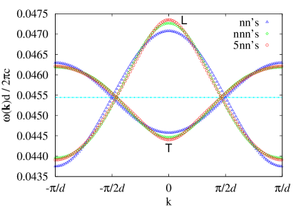
Figure 4: (Color online) Same as Fig. 3, but including three different numbers of neighbors: nearest-neighbors (nn’s), next-nearest-neighbors (nnn’s), and fifth-nearest-neighbors (5nn’s).

We have carried out similar calculations using other values of the parameter $\omega_{\text{p}}d/c$, namely $1.0$, $2.0$, and $5.0$. Such calculations are possible here because our calculations are non-quasistatic, so that the overlap integral between neighboring spheres falls off exponentially with separation. The results are given in Figs. 5, 7, and 9, respectively. The corresponding results including more overlap integrals are shown in Figs. 6, 8, and 10, respectively. It is also striking that, as $\omega_{\text{p}}d/c$ increases in going from Fig. 3 to Figs. 5, 7, and 9, the ratio $r_{\text{LT}}$ of the width of the L band to that of the T band steadily decreases. In Fig. 3, $r_{\text{LT}}>1$, in Fig. 9, $r_{\text{LT}}<1$, while in Fig. 7 (for which $\omega_{\text{p}}d/c=2.0$), $r_{\text{LT}}\sim 1$.

One could also say that, except for an overall scale factor, Fig. 9 looks like an inverted image of Fig. 3 about the horizontal line of $\omega_{\text{at}}$. The dispersion relations for the intermediate value $\omega_{\text{p}}d/c=2.0$ has nearly perfect symmetry about the horizontal line of $\omega_{\text{at}}$ (the T branches are nearly reflections of the L branch about the horizontal line of $\omega_{\text{at}}$), as in Fig. 7. For the nn case, the T and L bands cross at $\pm\pi/(2d)$, as can be seen in Figs. 3, 5, 7, and 9. When further neighbors are included, they cross at smaller values than $|\pi/(2d)|$, as can be seen in Figs. 6, 8, and 10, but the crossing points get closer to $\pm\pi/(2d)$ as $\omega_{\text{p}}$ increases. Also, the effects of including further neighbors become smaller as $\omega_{\text{p}}$ increases; they are smallest at $\omega_{\text{p}}d/c=5.0$, as can be seen in Fig. 10.

Figure 5: Same as Fig. 3, except $\omega_{\text{p}}d/c=1.0$ and $\omega_{\text{at}}d/(2\pi c)=0.1291$.

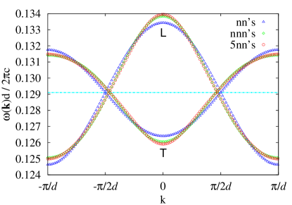
Figure 6: (Color online) Same as Fig. 4, except $\omega_{\text{p}}d/c=1.0$ and $\omega_{\text{at}}d/(2\pi c)=0.1291$.

Figure 7: Same as Fig. 3, except $\omega_{\text{p}}d/c=2.0$ and $\omega_{\text{at}}d/(2\pi c)=0.2537$.

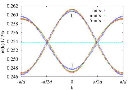
Figure 8: (Color online) Same as Fig. 4, except $\omega_{\text{p}}d/c=2.0$ and $\omega_{\text{at}}d/(2\pi c)=0.2537$.

Figure 9: Same as Fig. 3, except $\omega_{\text{p}}d/c=5.0$ and $\omega_{\text{at}}d/(2\pi c)=0.5691$.

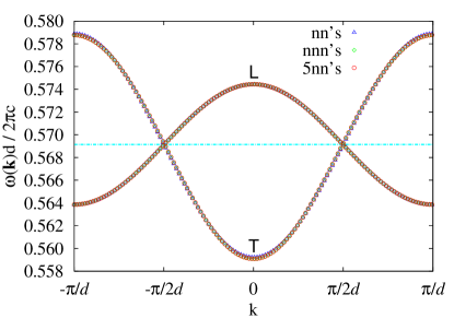
Figure 10: (Color online) Same as Fig. 4, except $\omega_{\text{p}}d/c=5.0$ and $\omega_{\text{at}}d/(2\pi c)=0.5691$.

Next we consider values of $R/d$ other than $1/3$, but still keeping the same value of $\omega_{1}=1.4\times 10^{15}\ \text{rad/s}$ (i.e., $\omega_{\text{p}}d/c=0.35$). For a smaller $R/d=0.25$, the variation of the band energies with $k$ becomes smaller, as seen in Fig. 11, than it is in Fig. 3, but the crossing points between the L and T branches still occur at $\pm\pi/(2d)$. This behavior becomes clearer when the results for several values of $R/d$ are plotted together as in Fig. 12. As $R/d$ increases, the variation of the band energies with $k$, and the separation between the L and T branches at both the zone center and zone boundary, increase, but the L and T branches still cross at $\pm\pi/(2d)$. If we include more neighbors up to fifth nearest-neighbors, but consider only up to $R/d=0.4$, we get the dispersion relations shown in Fig. 13. These show the same trends as in Fig. 12, except that the band crossing points occur at values of $|k|$ slightly less than $|\pi/(2d)|$. Furthermore, the separation between the L and T bands increases slightly at $k=0$, but decreases slightly at $k=\pm\pi/d$. We show only $R/d$ up to $0.4$ in this Figure because, in the quasistatic limit, there is evidence that for larger values of $R/d$ the dispersion relations are significantly modified by higher values of $\ell$.park

Figure 11: Same as Fig. 3, except that $R/d=0.25$ and $\omega_{\text{at}}d/(2\pi c)=0.04546$.

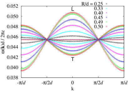
Figure 12: (Color online) Plotting together six different results for $\omega<\omega_{\text{p}}$, all with $\omega_{\text{p}}d/c=0.35$, but with different $R/d$: $R/d=0.33$ and $\omega_{\text{at}}d/(2\pi c)=0.04544$; $R/d=0.40$ and $\omega_{\text{at}}d/(2\pi c)=0.045426$; $R/d=0.45$ and $\omega_{\text{at}}d/(2\pi c)=0.045412$; $R/d=0.49$ and $\omega_{\text{at}}d/(2\pi c)=0.045399$; and $R/d=0.50$ and $\omega_{\text{at}}d/(2\pi c)=0.045396$. In each case, only nearest-neighbor overlaps are included.

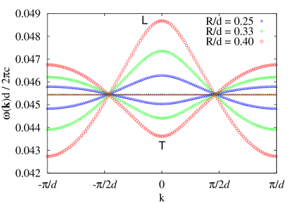
Figure 13: (Color online) Same as Fig. 12, except that only three $R/d$’s are plotted, with inclusion of up to the fifth nearest-neighbors. We omit the three largest values of $R/d$ because it may be necessary to include more than just $\ell=1$ when $R/d\gtrsim 0.4$.

IV Discussion

In this work we have calculated the photonic band structures of metal inverse opals and of a linear chain of spherical voids in a metallic host for frequencies below $\omega_{\text{p}}$, when $\ell=1$ using a tight-binding approximation. In both cases, we include only the $\ell=1$ “atomic” states of the voids. As a possible point of comparison, we have also computed the same band structures using the asymptotic forms of the spherical and modified spherical Bessel functions for small void radius. In this asymptotic region, there are only TM modes. The results for the linear chain of voids can be considered as the “inversions” of those in Ref. brongersma , in the sense discussed earlier. In other words, if we reflect our L and T branches with respect to the atomic energy level, we would get their L and T modes.

Although we did not discuss this approach, we did attempt to use the plane wave expansion method to calculate the band structure for the inverse opals, similarly to Refs. mcgurn and kuzmiak1 . Just as found in those papers, the photonic bands for modes below $\omega_{\text{p}}$ depend on the number of plane waves included in the expansion and on the type of field, $\mathbf{B}$ or $\mathbf{E}$, used in the expansion. Furthermore, this plane wave expansion method gives a large number of flat bands below $\omega_{\text{p}}$, which are difficult to interpret physically. Because of this problem, and because of the apparent non-convergence of this approach with the number of plane waves, we do not present these results here. By contrast, the band structures above $\omega_{\text{p}}$, when calculated using the plane wave expansion, varied smoothly with $\mathbf{k}$ and converged well with the number of plane waves included.

In calculating the tight-binding band structure for the linear chain (and the inverse opal structure), one should, in principle, include all the neighbors. But in practice, for the linear chain, it is sufficient to include only up to the fifth nearest-neighbors. This calculation is easily carried out, since the matrix in Eq. (39) is already diagonal in $x$, $y$, $z$ and the sum converges quickly. In fact, even the inclusion of neighbors beyond the first two sets changes the band structure very little. The smallness of the further neighbor effect is particularly apparent when $\omega_{\text{p}}d/c=5.0$, as in Fig. 10.

Although we studied the 3D and 1D lattices, we have not investigated a 2D lattice of spherical pores in a metallic host. For the 2D case, the matrix element $M_{\alpha,\beta}(\mathbf{R})$ can again be readily calculated using our tight-binding approximation. It is expected to have some nonzero off-diagonal elements in addition to the diagonal elements. Thus band structures somewhat similar to the 3D band structures shown in Fig. 2 are also expected in the 2D case.

In the quasistatic case, for metal grains in air, when $R/d$ is greater than about $0.4$, it becomes important to include more than just $\ell=1$ as in Ref. park . Inclusion of such higher $\ell$’s might be rather difficult in the present dynamical case, though it would be possible in the quasistatic limit for 1D chains of spherical nanopores.

In the present work, we have considered only the case of one cavity per primitive cell and $\ell=1$. It would be of a great interest to consider multiple cavities per unit cell. Of course, in this case, the dimension of the matrix in Eq. (39) will increase and the Bloch states in Eq. (41) will acquire an additional index. It should be straightforward to extend the present work to such a case, which would make an interesting subject for future work.

The surface effect of the metal nanopores on the eigenstates becomes prominent as the radius of a pore ($R$) or the ratio of radius to center-to-center separation ($R/d$) increases. Shockley surface states form on metal surfaces depending on the type of metal, such as the Fermi wavevector $k_{\text{F}}$ or the Fermi energy $\epsilon_{\text{F}}$. These surface states will interact with the eigenstates, resulting in the change of eigenvalues. However we think these effects are negligible, especially in the quasistatic limit since in the asymptotic limit, these oscillatory interactions take the formhyldgaard

$$E_{\text{pair}}^{\text{asym}}(a)\propto\left(\frac{4\epsilon_{\text{F}}}{\pi^{2}}\right)\frac{\sin(2k_{\text{F}}a+2\Theta)}{(k_{\text{F}}a)^{2}},$$ (64)

where $a$ is the interatomic separation, $\Theta$ is the effective interaction phase shift, $k_{\text{F}}$ the Fermi wavevector of the isotropic surface state, and $\epsilon_{\text{F}}$ the Fermi energy. The proportionality constant gives the consequences of scattering into bulk states.hyldgaard The very slow $a^{-2}$ decay of these interactions allows them to play a role at large separations, but the overall magnitude is small due to the sinusoidal term.

In summary, we have described a tight-binding method for calculating the photonic band structure of a periodic composite of spherical pores in a metallic host, and have applied it to both 1D and 3D systems. The method is fully dynamical, and is not limited to very small pores. The method does not have the convergence problems found when the magnetic or electric field is expanded in plane waves. Furthermore, there are no radiation losses to consider, unlike the complementary case of small metal particles in an insulating host, because the fields associated with these modes outside the pores are exponentially decaying. Thus, this method may be useful for a variety of periodic metal-insulator composites. It would be of interest to compare these calculations to experiments on such materials.

- (1) J. Q. Xia, Y. R. Ying, and S. H. Foulger, Adv. Mater. 17, 2463 (2005).
- (2) K. Busch and S. John, Phys. Rev. Lett. 83, 967 (1999).
- (3) Eli Yablonovitch, Phys. Rev. Lett. 58, 2059 (1987).
- (4) A. Scherer, O. Painter, B. D’Urso, R. Lee, and A. Yariv, J. Vac. Sci. Technol. B 16, 3906 (1998).
- (5) Attila Mekis, J. C. Chen, I. Kurland, Shanhui Fan, Pierre R. Villeneuve, and J. D. Joannopoulos, Phys. Rev. Lett. 77, 3787 (1996).
- (6) O. Painter, R. K. Lee, A. Scherer, A. Yariv, J. D. O’Brien, P. D. Dapkus, and I. Kim, Science 284, 1819 (1999).
- (7) F. Benabid, J. C. Knight, G. Antonopoulos, and P. St. J. Russell, Science 298, 399 (2002).
- (8) Y. Cao, J. O. Schenk, and M. A. Fiddy, Optics and Photonics Lett. 1, 1 (2008).
- (9) Arthur R. McGurn and Alexei A. Maradudin, Phys. Rev. B 48, 17576 (1993).
- (10) V. Kuzmiak, A. A. Maradudin, and F. Pincemin, Phys. Rev. B 50, 16835 (1994).
- (11) V. Kuzmiak and A. A. Maradudin, Phys. Rev. B 55, 7427 (1997).
- (12) I. H. H. Zabel and D. Stroud, Phys. Rev. B 48, 5004 (1993).
- (13) Mark L. Brongersma, John W. Hartman, and Harry A. Atwater, Phys. Rev. B 62, R16356 (2000).
- (14) Sung Yong Park and David Stroud, Phys. Rev. B 69, 125418 (2004).
- (15) W. H. Weber and G. W. Ford, Phys. Rev. B 70, 125429 (2004).
- (16) D. Gaillot, T. Yamashita, and C. J. Summers, Phys. Rev. B 72, 205109 (2005).
- (17) Ali E. Aliev, Sergey B. Lee, Anvar A. Zakhidov, and Ray H. Baughman, Physica C 453, 15 (2007).
- (18) See, e.g., J. D. Jackson, Classical Electrodynamics, 3rd ed. (Wiley, New York, 1999), pp. 374–376.
- (19) See, e.g., N. W. Ashcroft and N. D. Mermin, Solid State Physics (Saunders College Publishing, Orlando, 1976), pp. 189–190 (Problem 2) & pp. 184–185.
- (20) P. Hyldgaard and T. L. Einstein, Europhys. Lett. 59, 265 (2002); J. Cryst. Growth 275, e1637 (2005).