Integral equations in MHD: theory and application

$\dagger$Helmholtz-Zentrum Dresden-Rossendorf, P.O. Box 510119, D-01314 Dresden, Germany
$\ddagger$Shandong University, P. O. Box 88, Jing Shi Road 73 , Jinan City, Shandong Province, P. R. China

The induction equation of kinematic magnetohydrodynamics is mathematically equivalent to a system of integral equations for the magnetic field in the bulk of the fluid and for the electric potential at its boundary. We summarize the recent developments concerning the numerical implementation of this scheme and its applications to various forward and inverse problems in dynamo theory and applied MHD.

Keywords: Dynamo; integral equations; inverse problems

1 Introduction

This paper is intended as a summary and update of our recent work on the theoretical formulation, the numerical implementation, and the practical application of the integral equation approach (IEA) to kinematic magnetohydrodynamics (MHD). Actually, our activity in this field had started with the paper (Stefani et al., 2000), written together with Karl-Heinz Rädler, whom we would like to thank not only for his insistence on a rigorous mathematical formulation in this particular case, but also for many fruitful discussions over the course of time.

The theory of hydromagnetic dynamos is mainly concerned with the self-excitation of cosmic magnetic fields, with particular focus on the fields of planets, stars, and galaxies (Krause and Rädler 1980). As long as the self-excited magnetic field is weak and its influence on the velocity field is negligible we speak about the kinematic dynamo regime. When the magnetic field has grown to higher amplitudes the field-generating velocity field is modified, and the dynamo enters its saturation regime, which will not be considered in the present paper, though.

The familiar way to deal with kinematic dynamo action relies on the induction equation for the magnetic field B,

$${}\frac{\partial\textbf{B}}{\partial t}=\nabla\times(\textbf{u}\times\textbf{B})+\frac{1}{\mu_{0}\sigma}\Delta\textbf{B},\;\;\nabla\cdot\textbf{B}=0,$$ (1)

where u is considered as a pre-given velocity field, $\mu_{0}$ is the magnetic permeability constant, and $\sigma$ is electrical conductivity of the fluid. The time dependence of the magnetic field B in Eq. (1), in terms of exponential growth or decay, is governed by the ratio of field changes due to velocity gradients (first term on the r.h.s.) to the field dissipation (second term on the r.h.s.). This ratio is determined by the magnetic Reynolds number $R_{m}=\mu\sigma LU$, where $L$ and $U$ are typical length and velocity scales of the flow, respectively. When the magnetic Reynolds number reaches a critical value, denoted by $R_{m}^{c}$, the field can grow exponentially in time.

Equation (1) follows directly from pre-Maxwell’s equations and Ohm’s law in moving conductors. In order to make this equation solvable, boundary conditions of the magnetic field must be prescribed. In the case of vanishing excitations of the magnetic field from outside the considered finite region, the boundary condition of the magnetic field is given by $\textbf{B}=O(r^{-3})\;\mbox{as}\;r\rightarrow\infty$. For dynamos in spherical domains, as they are typical for planets and stars, the problem of implementing the non-local boundary conditions for the magnetic field is easily solved by using decoupled boundary conditions for each degree of the spherical harmonics. For other than spherically shaped dynamos, in particular for the recent laboratory dynamos working often in cylindrical domains, but also for dynamos in galaxies and planetesimals, the handling of the non-local boundary conditions is a notorious problem (Stefani et al. 2009).

A simple, but rather rude way to circumvent this problem is to replace the complicated non-local boundary conditions by simplified local ones (so-called ”vertical field conditions”). This method is sometimes used in the simulation of galactic dynamos (a recent example is Hubbard and Brandenburg 2010).

For the simulation of the cylindrical Karlsruhe dynamo experiment, Rädler et al. (1998, 2002) had used the alternative trick of embedding the actual electrically conducting dynamo domain into a sphere, and the region between this sphere and the surface of the dynamo was virtually filled by a medium of lower electrical conductivity. By reducing the value of this conductivity, it was possible to check the convergence of the numerical solution.

Of course, both methods are connected with losses of accuracy, the latter method being certainly more accurate. In order to fully implement the non-local boundary condition, Maxwell’s equations must be fulfilled in the exterior, too. This can be implemented in different ways. For the finite difference simulation of the Riga dynamo, a Laplace equation was solved, for each time-step, by a pseudo-relaxation method, in the exteriour of the dynamo domain and the magnetic field solutions in the interiour and in the exterior were matched using interface conditions (Stefani et al. 1999, Kenjereš et al. 2006). A similar method, although based on the finite element method, was developed by Guermond et al. (2003, 2007) and was intensively used later for practical dynamo applications (Guermond et al, 2009, Giesecke et al. 2010a, b, Nore et al. 2011).

A quite elegant technique to circumvent the solution in the exteriour was presented by Iskakov et al. (2004, 2005) who used a combination of a finite volume and a boundary element method. This latter method was recently used by Giesecke et al. (2008, 2010a, b) for the simulation of the French VKS-dynamo (although the main focus of that work laid on the particular effect of the high magnetic permeability impellers on the mode selection in this type of dynamo).

An alternative to the solution of the induction equation is the integral equation approach (IEA) for kinematic dynamos which basically relies on the self-consistent treatment of Biot-Savart’s law. For steady dynamo action in infinite domains of homogeneous conductivity, the IEA becomes very simple and had already been employed by a few authors (Gailitis 1970, Gailitis and Freibergs 1974, Dobler and Rädler 1998). For dynamo action in finite domains, however, the simple Biot-Savart equation has to be supplemented by a boundary integral equation for the electric potential (Roberts 1967, Stefani et al. 2000, Xu et al. 2004a). If the magnetic field becomes time-dependent, yet another equation for the vector potential can be added to get a closed system of integral equations (Xu et al. 2004b).

In the following section, we will present this formulation and its specifications in detail. Then we will consider its application to various dynamo problems, including those with different degrees of symmetry which enable dimensional reductions. At last, we will go over from forward problems to inverse problems for which the IEA represents an ideal mathematical starting point.

2 Mathematical formulation

Assume a fluid of electrical conductivity $\sigma$, flowing with velocity $\bf u$, to be confined in a finite region $V$ with boundary $S$, the exterior of this region consisting of insulating material (or vacuum). By further assuming the velocity $\bf u$ field to be stationary, we may write the electric field, the magnetic field and the magnetic vector potential in the following form:

$${\bf E}({\bf r},t)={\bf E}({\bf r})\exp{\lambda t},{\bf B}({\bf r},t)={\bf B}({\bf r})\exp{\lambda t},{\bf A}({\bf r},t)={\bf A}({\bf r})\exp{\lambda t},{}$$ (2)

where the real part of $\lambda$ is the growth rate, and its imaginary part is the frequency of the fields. In the general case, we allow external currents to be present that produce a magnetic field ${\bf B}_{0}$. The remaining magnetic field, induced by the flow, is denoted by $\bf b$. Then, the current density is governed by Ohm’s law

$${}{\bf j} = \sigma({\bf E}+{\bf u}\times({\bf B}_{0}+{\bf b}))$$ (3)

$$= \sigma(-\nabla\phi-\lambda{\bf A}+{\bf u}\times({\bf B}_{0}+{\bf b}))$$

where the electric field E, the electric potential $\phi$ and the magnetic vector potential $\bf A$ are used. Applying now Biot-Savart’s law to the magnetic field, Green’s second theorem to the solution of the Poisson equation for the electric potential, and Helmholtz’s theorem for the integral representation of the vector potential in terms of the magnetic field, we arrive at the following integral equation system:

$${\mathbf{b}}({\mathbf{r}}) = \frac{\mu\sigma}{4\pi}\int_{V}\frac{({\mathbf{u}}({\mathbf{r}}^{\prime})\times({\mathbf{B}}_{0}({\mathbf{r}}^{\prime})+{\mathbf{b}}({\mathbf{r}}^{\prime})))\times({\mathbf{r}}-{\mathbf{r}}^{\prime})}{|{\mathbf{r}}-{\mathbf{r}}^{\prime}|^{3}}dV^{\prime}$$ (4)

$$-\frac{\mu\sigma\lambda}{4\pi}\int_{V}\frac{{\mathbf{A}}({\mathbf{r}}^{\prime})\times({\mathbf{r}}-{\mathbf{r}}^{\prime})}{|{\mathbf{r}}-{\mathbf{r}}^{\prime}|^{3}}dV^{\prime}-\frac{\mu\sigma}{4\pi}\int_{S}\phi({\mathbf{s}}^{\prime}){\mathbf{n}}({\mathbf{s}}^{\prime})\times\frac{{\mathbf{r}}-{\mathbf{s}}^{\prime}}{|{\mathbf{r}}-{\mathbf{s}}^{\prime}|^{3}}dS^{\prime}$$

$$\frac{1}{2}\phi({\mathbf{s}}) = \frac{1}{4\pi}\int_{V}\frac{({\mathbf{u}}({\mathbf{r}}^{\prime})\times({\mathbf{B}}_{0}({\mathbf{r}}^{\prime})+{\mathbf{b}}({\mathbf{r}}^{\prime})))\cdot({\mathbf{s}}-{\mathbf{r}}^{\prime})}{|{\mathbf{s}}-{\mathbf{r}}^{\prime}|^{3}}dV^{\prime}$$ (5)

$$-\frac{\lambda}{4\pi}\int_{V}\frac{{\mathbf{A}}({\mathbf{r}}^{\prime})\cdot({\mathbf{s}}-{\mathbf{r}}^{\prime})}{|{\mathbf{s}}-{\mathbf{r}}^{\prime}|^{3}}dV^{\prime}-\frac{1}{4\pi}\int_{S}\phi({\mathbf{s}}^{\prime}){\mathbf{n}}({\mathbf{s}}^{\prime})\cdot\frac{{\mathbf{s}}-{\mathbf{s}}^{\prime}}{|{\mathbf{s}}-{\mathbf{s}}^{\prime}|^{3}}dS^{\prime}$$

$${\mathbf{A}}({\mathbf{r}}) = \frac{1}{4\pi}\int_{V}\frac{({\mathbf{B}}_{0}({\mathbf{r}}^{\prime})+{\mathbf{b}}({\mathbf{r}}^{\prime}))\times({\mathbf{r}}-{\mathbf{r}}^{\prime})}{|{\mathbf{r}}-{\mathbf{r}}^{\prime}|^{3}}dV^{\prime}$$ (6)

$$+\frac{1}{4\pi}\int_{S}{\mathbf{n}}({\mathbf{s}}^{\prime})\times\frac{{\mathbf{B}}_{0}({\mathbf{s}}^{\prime})+{\mathbf{b}}({\mathbf{s}}^{\prime})}{|{\mathbf{r}}-{\mathbf{s}}^{\prime}|}dS^{\prime},$$

where $\mu$ is the permeability of the fluid.

Note that this integral equation system is by far not the only possible one. The double use of the magnetic field and its vector potential might even seem a bit awkward. There are indeed other possible schemes, one of them starting from the Helmholtz equation for the vector potential which leads, however, to a nonlinear eigenvalue problem in $\lambda$ (see Dobler and Rädler 1998), while the above scheme is a linear eigenvalue in $\lambda$ which has many advantages when it comes to the numerical treatment.

The general integral equation system (4-6) can now be further specified. In the case with ${\bf B}_{0}\neq 0$ and small $R_{m}$, i.e. below the threshold of self-excitation, the system describes an induction problem in which the applied field ${\bf B}_{0}$ is only slightly deformed by the velocity. In the case of ${\bf B}_{0}=0$, the system represents an eigenvalue problem for the complex constant $\lambda$, with only negative eigenvalues for small $R_{m}$ (below the dynamo threshold), and one or a few eigenvalues with positive real parts for the case of large $R_{m}$ (above the dynamo threshold).

In the case of a steady problem, with neither any growth/decay nor any oscillation of the field, this equation system reduces to

$${\mathbf{b}}({\mathbf{r}}) = \frac{\mu\sigma}{4\pi}\int_{V}\frac{({\mathbf{u}}({\mathbf{r}}^{\prime})\times({\mathbf{B}}_{0}({\mathbf{r}}^{\prime})+{\mathbf{b}}({\mathbf{r}}^{\prime})))\times({\mathbf{r}}-{\mathbf{r}}^{\prime})}{|{\mathbf{r}}-{\mathbf{r}}^{\prime}|^{3}}dV^{\prime}$$ (7)

$$-\frac{\mu\sigma}{4\pi}\int_{S}\phi({\mathbf{s}}^{\prime}){\mathbf{n}}({\mathbf{s}}^{\prime})\times\frac{{\mathbf{r}}-{\mathbf{s}}^{\prime}}{|{\mathbf{r}}-{\mathbf{s}}^{\prime}|^{3}}dS^{\prime}$$

$$\frac{1}{2}\phi({\mathbf{s}}) = \frac{1}{4\pi}\int_{V}\frac{({\mathbf{u}}({\mathbf{r}}^{\prime})\times({\mathbf{B}}_{0}({\mathbf{r}}^{\prime})+{\mathbf{b}}({\mathbf{r}}^{\prime})))\cdot({\mathbf{s}}-{\mathbf{r}}^{\prime})}{|{\mathbf{s}}-{\mathbf{r}}^{\prime}|^{3}}dV^{\prime}$$ (8)

$$-\frac{1}{4\pi}\int_{S}\phi({\mathbf{s}}^{\prime}){\mathbf{n}}({\mathbf{s}}^{\prime})\cdot\frac{{\mathbf{s}}-{\mathbf{s}}^{\prime}}{|{\mathbf{s}}-{\mathbf{s}}^{\prime}|^{3}}dS^{\prime}.$$

Again, we can distinguish the case with ${\bf B}_{0}\neq 0$ and small $R_{m}$ for which it represent a stationary induction problem. This is of particular interest for many technical liquid metal problems (steel casting, crystal growth) characterized by a rather small $R_{m}$. In this case, the induced field $\bf b$ can be omitted under the integrals which leads to a linear relation between the source $\bf u$ and the result $\bf b$ of the induction process. This linear relationship represents a convenient starting point for the treatment of the inverse problem to infer $\bf u$ in the bulk of the fluid from values of $\bf b$ measured in the exteriour of the fluid. A problem of this sort will be discussed in the next but one section. In the case of ${\bf B}_{0}=0$, the steady system represents again an eigenvalue problem, but now for the critical $R_{m}$ that leads to a marginal and non-oscillatory dynamo.

3 Numerical implementation and dimensional reductions

In this section we will illustrate the general method by treating dynamo problems first in 3D and then in 2D and 1D, the latter cases being characterized by different degrees of symmetries that can be exploited for a dimensional reduction of the problem. We will see that, in stark contrast to the corresponding procedure in the differential equation approach, such a dimensional reduction represents a formidable task in the IEA.

3.1 3D - Matchbox dynamos

Let us start with a full problem in 3D for which we will summarize the result of the papers (Xu et al. 2004a, 2004b) for a so-called ”matchbox dynamo”, i.e. a mean-field dynamo in a rectangular box. The original assumption of a full velocity field as the source of induction can be easily translated to the case with a helical turbulence parameter $\alpha$. Assume that we apply a specific spatial discretization of all fields in Eqs. (4-6), we formally obtain

$$b_{i} = \mu\sigma[P_{ik}(B_{0k}+b_{k})-\lambda R_{ij}A_{j}-Q_{il}\phi_{l}],$$ (9)

$$G_{ml}\phi_{l} = S_{mk}(B_{0k}+b_{k})-\lambda T_{mj}A_{j},$$ (10)

$$A_{j} = W_{jk}(B_{0k}+b_{k}),$$ (11)

where Einstein’s summation convention is assumed. We have used the notion $G_{ml}=0.5\,\delta_{ml}+U_{ml}$. $B_{0k}$ and $b_{k}$ denote the degrees of freedom of the externally added magnetic field and the induced magnetic field, $A_{j}$ the degrees of freedom of the vector potential in the volume $V$, $\phi_{l}$ the degrees of freedom of the electric potential at the boundary surface. For the later numerical utilization with different induction sources it is useful that only the matrices $P_{ik}$ and $S_{mk}$ depend on the velocity (or on the corresponding mean-field induction sources), while $R_{ij}$, $Q_{il}$, $T_{mj}$, $G_{ml}$ and $W_{jk}$ depend only on the geometry of the dynamo domain and on the details of the discretization.

Inserting Eqs. (10) and (11) into Eq. (9), which eliminates $A_{j}$ and $\phi_{l}$, we end up with one single matrix equation for the induced magnetic field components $b_{i}$:

$${}b_{i} = \mu\sigma[P_{ik}(B_{0k}+b_{k})-\lambda R_{ij}W_{jk}(B_{0k}+b_{k})-Q_{il}G_{lm}^{-1}S_{mk}(B_{0k}+b_{k})$$ (12)

$$+\lambda Q_{il}G_{lm}^{-1}T_{mj}W_{jk}(B_{0k}+b_{k})]$$

which can be further transformed into

$${}[\delta_{ik}-\mu\sigma E_{ik}-\mu\sigma\lambda F_{ik}]b_{k}=[\mu\sigma E_{ik}+\mu\sigma\lambda F_{ik}]B_{0k},$$ (13)

where $E_{ik}=P_{ik}-Q_{il}G_{lm}^{-1}S_{mk}$ and $F_{ik}=-R_{ij}W_{jk}+Q_{il}G_{lm}^{-1}T_{mj}W_{jk}$. It should be noted, though, that the needed inversion of the boundary integral equation (10) for the electric potential needs some specific care (Wondrak et al. 2009). This has to do with the singular character of this equation which, in turn, mirrors the ambiguity of the electric potential with respect to some additive constant.

For the computation of induction effects, the induced magnetic field can be obtained by solving the algebraic equation system (12). In order to compute kinematic dynamos without external sources, Eq.(12) reduces to the following generalized eigenvalue problem for $\lambda$:

$${}[\delta_{ik}-\mu\sigma E_{ik}]b_{k}=\lambda\mu\sigma F_{ik}b_{k},$$ (14)

To test the working of the scheme we apply it now to $\alpha^{2}$ dynamos in rectangular geometry, which we would like to coin ”matchbox dynamos”. As usual in mean-field dynamo theory (see Krause and Rädler 1980), $\alpha$ parametrizes the induction effect of helical turbulence on the large scale magnetic field. Formally speaking, the term ${\bf u}\times{\bf B}$ in the electromotive force term in Eq. (3) has to be replaced by $\alpha\cdot{\bf B}$.

While the spherically symmetric $\alpha^{2}$ dynamo has played a paradigmatic role in dynamo theory, its counterpart in rectangular geometry is certainly a highly artificial problem without any application in astrophysics. Nevertheless, it may illustrate the capabilities of the IEA to solve dynamo problems in geometries that are far away from spherical.

In our specific example (for more cases see Xu et al. 2004b) we consider a homogeneous distribution, $\alpha({\bf r})=C$, in a ”matchbox” with side lengths 2.0x1.6x1.2 which gives approximately the same volume as a corresponding sphere of radius 1. The domain is divided into $10^{3}$ smaller rectangular boxes, with each face divided into $10^{2}$ rectangles.

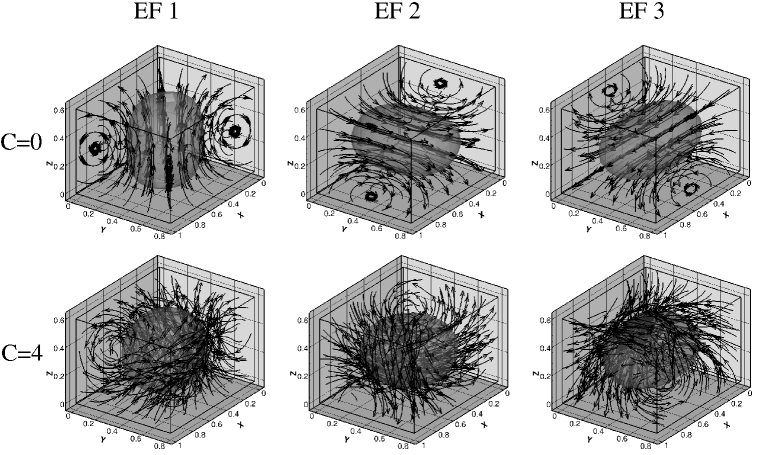
Figure 1: Magnetic eigenfields corresponding to the three dominant eigenvalues of the $\alpha^{2}$ dynamo in a matchbox with sidelengthes ratio 2x1.6x1.2.

For this setting, we find the first three critical values of $C$ to be $C^{\prime}_{1}=4.728$, $C^{\prime}_{2}=4.898$, and $C^{\prime}_{3}=4.934$. The corresponding first three eigenfunctions are shown, for the free decay case $C=0$ and the slightly sub-critical case $C=4$, in figure 1. These eigenfunctions still resemble the corresponding eigenfunctions in the spherical case. However, the exact degeneracy of the eigenvalues in the latter case is lifted now. The lowest eigenvalue corresponds to an eigenfunction whose dipolar axis is perpendicular to the largest face. Nevertheless, the three eigenvalues are still close the well-known value 4.49 for the spherical case.

3.2 2D - VKS-like dynamos

The recent successful dynamo experiments (see Stefani et al. 2008 for a recent survey) in Riga (Gailitis et al. 2000), Karlsruhe (Stieglitz and Müller 2001), and Cadarache (Monchaux et al. 2009) were all carried out in cylindrical vessels filled with liquid sodium. For this reason it is worth to specify the integral equation approach to this geometry. As long as the dynamo source (i.e. the velocity field or a corresponding mean-field quantity) is axisymmetric, the different azimuthal modes of the electromagnetic fields with the angular dependence according to $\exp(im\varphi)$ can be decoupled. Ultimately, this leads to a tremendous reduction of the numerical effort. The price we have to pay for this is the necessity to carefully deriving the dimensionally reduced version of the integral equation system. The necessary integrations over $\varphi$ turnes out to be a formidable task (see Xu et al. 2008), quite in contrast to the respective procedure in the differential equation approach, where the expression $\partial/\partial\varphi$ can simply replaced by $im$.

Lets assume now the electrically conducting fluid to be confined in a cylinder with radius $R$ and total height $2H$. Introducing the cylindrical coordinate system ($\rho,\varphi,z$), we have

$${\mathbf{r}}=[\rho\cos\varphi,\rho\sin\varphi,z]^{T},{\mathbf{b}}=[b_{\rho},b_{\varphi},b_{z}]^{T},{\mathbf{u}}=[u_{\rho},u_{\varphi},u_{z}]^{T}.$$ (15)

The magnetic field ${\mathbf{b}}$, the electric potential $\phi$, and the vector potential ${\mathbf{A}}$ all are expanded into azimuthal modes:

$${}\pmatrix{{\mathbf{b}}\cr\phi\cr{\mathbf{A}}}=\sum_{m=-\infty}^{\infty}\pmatrix{{\mathbf{b}}_{m}\cr\phi_{m}\cr{\mathbf{A}}_{m}}\exp(im\varphi).$$ (16)

As long as the velocity field is axisymmetric (i.e. it has only a component with $m=0$), the fields $[{\mathbf{b}}_{m},\phi_{m},{\mathbf{A}}_{m}]^{T}$ with different $m=0,\pm 1,\pm 2,\cdots$ decouple from each other. For the sake of convenience, we will always re-denote $[{\mathbf{b}}_{m},\phi_{m},{\mathbf{A}}_{m}]^{T}$ as $[{\mathbf{b}},\phi,{\mathbf{A}}]^{T}$. The reduction to a problem exclusively in $r$ and $z$ is then achieved by carrying out all integrations over $\phi$. This painstaking procedure results finally in the following system of matrix equations

$$\pmatrix{{{b}}_{\rho}\cr{{b}}_{\varphi}\cr{{b}}_{z}\cr} = \mu\sigma\left[{\mathbf{P}}\pmatrix{{{B}}_{0\rho}+{{b}}_{\rho}\cr{{B}}_{0\varphi}+{{b}}_{\varphi}\cr{{B}}_{0z}+b_{z}}-{\mathbf{Q}}\pmatrix{{{\phi}}_{s1}\cr{{\phi}}_{s2}\cr{{\phi}}_{s3}}-\lambda{\mathbf{R}}\pmatrix{{{A}}_{\rho}\cr{{A}}_{\varphi}\cr{{A}}_{z}\cr}\right],$$ (17)

$$\frac{1}{2}\pmatrix{{\mathbf{\phi}}_{s1}\cr{\mathbf{\phi}}_{s2}\cr{\mathbf{\phi}}_{s3}} = {\mathbf{S}}\pmatrix{{{B}}_{0\rho}+{{b}}_{\rho}\cr{{B}}_{0\varphi}+{{b}}_{\varphi}\cr{{B}}_{0z}+b_{z}}-\lambda{\mathbf{T}}\pmatrix{{{A}}_{\rho}\cr{{A}}_{\varphi}\cr{{A}}_{z}}-{\mathbf{U}}\pmatrix{{\mathbf{\phi}}_{s1}\cr{{\phi}}_{s2}\cr{{\phi}}_{s3}},$$ (18)

$$\pmatrix{{{A}}_{\rho}\cr{{A}}_{\varphi}\cr{{A}}_{z}} = {\mathbf{W}}\pmatrix{{{B}}_{0\rho}+{{b}}_{\rho}\cr{{B}}_{0\varphi}+{{b}}_{\varphi}\cr{{B}}_{0z}+b_{z}\cr},$$ (19)

where the matrix elements of $\mathbf{P}$, $\mathbf{Q}$, $\mathbf{R}$, $\mathbf{S}$, $\mathbf{T}$, $\mathbf{U}$, and $\mathbf{W}$ can be found in the paper by Xu et al. (2008). Combining Eqs.(17-19), we obtain

$${}({\mathbf{I}}-\mu\sigma{\mathbf{E}}-\mu\sigma\lambda{\mathbf{F}}){\mathbf{b}}=\mu\sigma({\mathbf{E}}+\lambda{\mathbf{F}}){\mathbf{B}}_{0},$$ (20)

where

$${\mathbf{E}} = {\mathbf{P}}-{\mathbf{Q}}\cdot(\frac{1}{2}{\mathbf{I}}+{\mathbf{U}})^{-1}\cdot{\mathbf{S}}$$ (21)

$${\mathbf{F}} = {\mathbf{Q}}\cdot(\frac{1}{2}{\mathbf{I}}+{\mathbf{U}})^{-1}\cdot{\mathbf{T}}\cdot{\mathbf{W}}-{\mathbf{R}}\cdot{\mathbf{W}}\;.$$ (22)

Again, induced magnetic fields can be obtained by solving the algebraic equation system (20), while for kinematic dynamo problems, the generalized eigenvalue problem

$${}({\mathbf{I}}-\mu\sigma{\mathbf{E}})\cdot{\mathbf{b}}=\mu\sigma\lambda{\mathbf{F}}\cdot{\mathbf{b}}$$ (23)

has to be solved.

In connection with the optimization of the VKS dynamo experiment, Marié, Normand and Daviaud (2006) had studied an analytical test flow of the same topological type as the flow in the real experiment (flow topology s2⁺t2, what means two poloidal eddies with radial inflow in the equatorial plane, together with two counter-rotating toroidal eddies). The velocity field of this ”MND flow” reads:

$$u_{r} = -\frac{\pi}{2}\;r\;(1-r)^{2}(1+2r)\cos(\pi z)$$ (24)

$$u_{\varphi} = 4\epsilon r(1-r)\sin(\pi z/2)$$ (25)

$$u_{z} = (1-r)(1+r-5r^{2})\sin(\pi z).$$ (26)

For the parameter $\epsilon$, which determines the ratio of toroidal to poloidal flow, we have used the value $\epsilon=0.7259$. For the case without any side layer, the structure of the magnetic eigenfield is illustrated in figure 2. In figure 2a the field lines of the equatorial dipole are seen, while the isosurfaces of the magnetic field energy (figure 2b) show the typical banana-like structure.

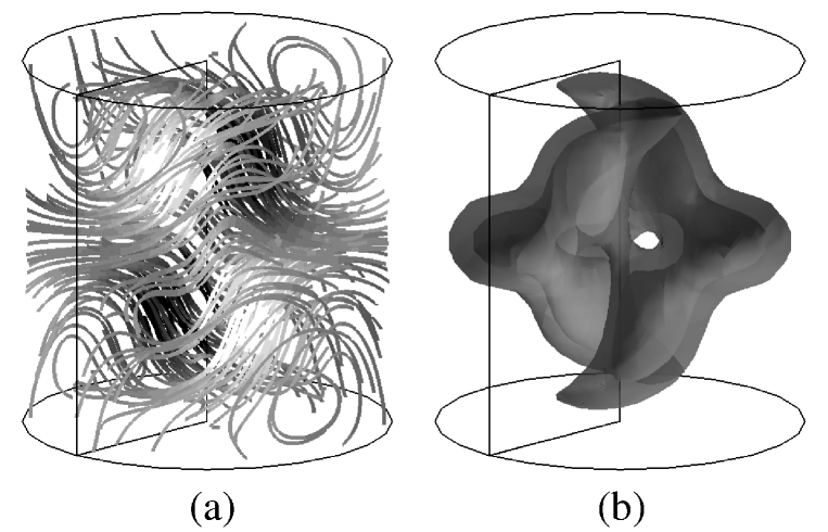
Figure 2: Simulated magnetic field structure of the dominant eigenmode of the MND flow. (a) Magnetic field lines of the equatorial dipole field. (b) Iso-surface of the magnetic field energy.

3.3 Reduction to 1D - Spherically symmetric $\alpha^{2}$ dynamo

After having utilized, in the former subsection, the cylindrical symmetry of some flow field for reducing the full 3D IEA system to a 2D system, we go now one step further and invoke spherical symmetry to make a reduction to a 1D problem. This is possible for a spherically symmetric $\alpha^{2}$ dynamo. In contrast to the original, analytically solvable model with constant $\alpha$ (Krause and Rädler 1980), we will allow the profile $\alpha$ to vary with the radial coordinate $r$. After summarizing the derivation of the two coupled radial integral equations as given in (Stefani et al. 2000, Xu et al. 2004b), we will treat numerically a non-trivial model with a radial dependence $\alpha(r)=Cr^{2}$.

The divergence-free magnetic field $\bf{B}$ is split, as usual in dynamo theory, into a poloidal and a toroidal part, denoted by ${\bf{B}}_{P}$ and ${\bf{B}}_{T}$. Using the Coulomb gauge, $\nabla\cdot{\bf A}=0$, the same can be done for the vector potential, ${\bf A}={\bf{A}}_{P}+{\bf{A}}_{T}$. All these fields can be represented by the defining scalars $S$, $T$, $S^{A}$, $T^{A}$ according to

$${}{\bf{B}}_{P}=\nabla\times\nabla\times\left(\frac{S}{r}\,{\bf{r}}\right),\;\;\;{\bf{B}}_{T}=\nabla\times\left(\frac{T}{r}\,{\bf{r}}\right)\;,$$ (27)

$${}{\bf{A}}_{P}=\nabla\times\nabla\times\left(\frac{S^{A}}{r}\,{\bf{r}}\right),\;\;\;{\bf{A}}_{T}=\nabla\times\left(\frac{T^{A}}{r}\,{\bf{r}}\right)\;.$$ (28)

For our spherical problem, the defining scalars and the electric potential can be expanded in series of spherical harmonics $Y_{lm}(\theta,\phi)$. As an example we indicate

$${}S(r,\theta,\phi) = \sum_{l,m}s_{lm}(r)Y_{lm}(\theta,\phi)\;,$$ (29)

and corresponding expressions can be written for $T(r,\theta,\phi)$, $S^{A}(r,\theta,\phi)$, $T^{A}(r,\theta,\phi)$ and $\varphi(r,\theta,\phi)$, with $s_{lm}(r)$ being replaced by $t_{lm}(r)$, $s^{A}_{lm}(r)$, $t^{A}_{lm}(r)$, and $\varphi_{lm}(r)$, respectively.

For the spherical harmonics $Y_{lm}(\theta,\phi)$ the definition

$${}Y_{lm}(\theta,\phi)=\sqrt{\frac{2l+1}{4\pi}\frac{(l-m)!}{(l+m)!}}\;P_{lm}(\cos\theta)e^{im\phi}\$$ (30)

is employed, which implies the following orthogonality relation for the $Y_{lm}(\theta,\phi)$:

$${}\int_{0}^{2\pi}d\phi\int_{0}^{\pi}\sin\theta\,d\theta\,Y_{l^{\prime}m^{\prime}}^{\ast}(\theta,\phi)Y_{lm}(\theta,\phi)=\delta_{ll^{\prime}}\delta_{mm^{\prime}}\;.$$ (31)

From Eqs. (27-29) we obtain the components of $\bf{B}$ in the form

$$B_{r}(r,\theta,\phi) = \sum\limits_{l,m}\frac{l(l+1)}{r^{2}}s_{lm}(r)Y_{lm}(\theta,\phi)$$ (32)

$$B_{\theta}(r,\theta,\phi) = \sum\limits_{l,m}\left(\frac{t_{lm}(r)}{r\sin\theta}\frac{\partial Y_{lm}(\theta,\phi)}{\partial\phi}+\frac{1}{r}\frac{ds_{lm}(r)}{dr}\frac{\partial Y_{lm}(\theta,\phi)}{\partial\theta}\right)$$ (33)

$$B_{\phi}(r,\theta,\phi) = \sum\limits_{l,m}\left(-\frac{t_{lm}(r)}{r}\frac{\partial Y_{lm}(\theta,\phi)}{\partial\theta}+\frac{1}{r\sin\theta}\frac{ds_{lm}(r)}{dr}\frac{\partial Y_{lm}(\theta,\phi)}{\partial\phi}\right)\;,$$ (34)

and equivalent expressions for the components of $\bf A$, in which $s_{lm}(r)$ and $t_{lm}(r)$ are replaced by $s^{A}_{lm}(r)$ and $t^{A}_{lm}(r)$, respectively.

A necessary ingredient for the dimensional reduction is the expression for the inverse distance between two points $\bf{r}$ and $\bf{r^{\prime}}$ in terms of spherical harmonics,

$${}\frac{1}{|{\bf{r}}-{\bf{r^{\prime}}}|}=4\pi\sum_{l=0}^{\infty}\sum_{m=-l}^{l}\frac{1}{2l+1}\frac{r_{<}^{l}}{r_{>}^{l+1}}Y_{lm}^{\ast}(\theta^{\prime},\phi^{\prime})Y_{lm}(\theta,\phi)\;,$$ (35)

where $r_{>}$ denotes the larger of the values $r$ and $r^{\prime}$, and $r_{<}$ the smaller one.

On this basis, the two coupled integral equations for the functions $s_{lm}(r)$ and $t_{lm}(r)$ can be derived. The first equation for $s_{lm}(r)$ can easily be obtained by multiplying the magnetic field with the unit vector in radial direction and then integrating over the angles $\theta$ and $\phi$. The derivation of the equation for $t_{lm}(r)$ needs more work, including the treatment of the electric potential and the vector potential at the boundary.

Here we go straight to the final result of this procedure, whose details were worked out by Xu et al (2004b): $s_{lm}(r)$ and $t_{lm}(r)$:

$${}s_{lm}(r) = \frac{\mu_{0}\sigma}{2l+1}\left[\int_{0}^{r}\frac{{r^{\prime}}^{l+1}}{r^{l}}\,\alpha(r^{\prime})\,t_{lm}(r^{\prime})\,dr^{\prime}+\int_{r}^{R}\frac{r^{l+1}}{{r^{\prime}}^{l}}\,\alpha(r^{\prime})\,t_{lm}(r^{\prime})\,dr^{\prime}\right.$$ (36)

$$\left.-\lambda\int_{0}^{r}\frac{{r^{\prime}}^{l+1}}{r^{l}}s_{lm}(r^{\prime})dr^{\prime}-\lambda\int_{r}^{R}\frac{r^{l+1}}{{r^{\prime}}^{l}}s_{lm}(r^{\prime})dr^{\prime}\right]\;.\$$

and

$${}t_{lm}(r) = \mu_{0}\sigma\left[\alpha(r)s_{lm}(r)-\frac{l+1}{2l+1}\int_{0}^{r}\frac{d\alpha(r^{\prime})}{dr^{\prime}}s_{lm}(r^{\prime})\frac{{r^{\prime}}^{l}}{r^{l}}dr^{\prime}\right.$$ (37)

$$+\frac{l}{2l+1}\int_{r}^{R}\frac{d\alpha(r^{\prime})}{dr^{\prime}}s_{lm}(r^{\prime})\frac{r^{l+1}}{{r^{\prime}}^{l+1}}dr^{\prime}+\frac{l+1}{2l+1}\frac{r^{l+1}}{R^{2l+1}}\int_{0}^{R}{r^{\prime}}^{l}\frac{d\alpha(r^{\prime})}{dr^{\prime}}s_{lm}(r^{\prime})dr^{\prime}$$

$$+\frac{\lambda}{2l+1}\frac{r^{l+1}}{R^{2l+1}}\int_{0}^{R}{r^{\prime}}^{l+1}t_{lm}(r^{\prime})dr^{\prime}-\frac{\lambda}{2l+1}\int_{0}^{r}\frac{{r^{\prime}}^{l+1}}{r^{l}}t_{lm}(r^{\prime})dr^{\prime}$$

$$\left.-\frac{\lambda}{2l+1}\int_{r}^{R}\frac{r^{l+1}}{{r^{\prime}}^{l}}t_{lm}(r^{\prime})dr^{\prime}-\frac{r^{l+1}}{R^{l+1}}\alpha(R)s_{lm}(R)]\right]\;.$$

The correctness of this system can be easily checked by differentiating equations (36) and (37) two times with respect to the radius which gives the two well-known differential equations for $s_{lm}(r)$ and $t_{lm}(r)$:

$${}\lambda s_{lm}=\frac{1}{\mu_{0}\sigma}\left[\frac{d^{2}s_{lm}}{dr^{2}}-\frac{l(l+1)}{r^{2}}s_{lm}\right]+\alpha(r)t_{lm},$$ (38)

$${}\lambda t_{lm}=\frac{1}{\mu_{0}\sigma}\left[\frac{d^{2}t_{lm}}{dr^{2}}-\frac{l(l+1)}{r^{2}}t_{lm}\right]-\frac{d}{dr}\left(\alpha(r)\frac{ds_{lm}}{dr}\right)+\frac{l(l+1)}{r^{2}}\alpha(r)s_{lm},$$ (39)

with the boundary conditions

$${}\left.t_{lm}(R)=R\frac{ds_{lm}(r)}{dr}\right|_{r=R}+ls_{lm}(R)=0.$$ (40)

It should be noted that in this particular case the complicated dimensional reduction (by expressing the fields in spherical harmonics and integrating over the spherical angles) can be circumvented by a simpler one. This starts directly from the differential equation system (38-40) for which the Green functions can be derived which then lead to the integral equation system (36-37) (Xu et al.2004b).

Now we turn to the numerical utilization of the radial integral equation system (36-37). The discretization in radial direction was done with a grid number of 128 which gives already a satisfactory accuracy. The eigenvalue solver gives us immediately all the eigenvalues. This is illustrated in figure 3, which shows for the case $\alpha(r)=Cr^{2}$ the real part (figure 3a) and the imaginary part (figure 3b) of the first 8 eigenvalues. The existence of two so-called exceptional points, at which two real eigenvalue branches coalesce and continue as a pair of complex conjugated eigenvalues, is clearly seen.

Figure 3: Eigenvalues of the spherically symmetric $\alpha$ dynamo with a radial dependence $\alpha(r)=Cr^{2}$. (a) Growth rates. (b) Frequencies.

4 Inverse problems for small $R_{m}$

Assuming a velocity field as given, and asking for the resulting magnetic field, represents a typical forward problem. The question can, however, also be inverted: assume the magnetic field as being measured in the exteriour of the fluid, what is the velocity that produces this field? This is a typical inverse problem, and it has puzzled dynamo theorist since many years.

In the general case, for arbitrary values of $R_{m}$, it represents a highly nonlinear inverse problem. Some progress in its treatment has been made for restricted set-ups, for example by applying the so-called frozen-flux approximation for the Earth’s core which allows to determine (still with some appropriate regularization) solutions for the tangential velocity field components at the Core-Mantel boundary from the measured time dependence of the radial magnetic field components (Roberts and Scott 1965). A complementary sort of restricted models is concerned with the determination of the radial dependence of $\alpha(r)$ of an assumed spherically symmetric $\alpha^{2}$ model from spectral properties. Solving such a type of restricted inverse problems (by means of an Evolutionary Strategy) it was possible, e.g., to obtain such $\alpha$ profiles that lead to oscillatory dynamo solutions (Stefani and Gerbeth 2003). Apart from those special solutions, inverse dynamo theory is still in its infancy.

The situation becomes much better for the case of induction problems with small $R_{m}$. As mentioned above the induced field $\bf b$ can then be omitted under the integrals, and we obtain a linear relation between the (wanted) source $\bf u$ and the (measured) result $\bf b$ of the induction process.

Although it is far from being a generic geo- or astrophysical problem, we would like to illustrate the typical solution procedure of such inverse problems by a model related to industrial steel casting. Figure 4a shows the set-up of a corresponding model experiment in which a liquid metal (in our case GaInSn) is poured from a tundish through an submerged entry nozzle into the mould. Among other problems of industrial interest, like flow instabilities due to Argon entrainment into the metal, we deal here with the problem how a magnetic stirrer can influence the flow structure in the mould. For this purpose, we use a so-called one-port submerged entry nozzle with just a hole at the bottom of the nozzle.

Based on the integral equation system (7-8), specified to small $R_{m}$, we have developed the so-called Contactless Inductive Flow Tomography (CIFT) for the reconstruction of velocity fields from externally measured magnetic fields (Stefani and Gerbeth 1999, 2000a, b, Stefani et al. 2004). While CIFT is in principle able to infer full 3D velocity fields by applying subsequently two different (e.g. orthogonal) external magnetic fields, for the present case of thin slab casting it can be reduced to the determination of the velocity components parallel to the wide faces of the mould (Wondrak et al. 2010). For this it is enough to apply only one magnetic field by a single coil (see figure 4a). The interaction of the flow with the applied field produces induced magnetic fields that we measure at a number of positions at the narrow faces of the mould in order to reconstruct from them the velocity field. The mathematics of this inversion relies in the minimization of the mean squared deviation of the measured magnetic fields from the fields resulting according to the integral equation system (7-8) from the velocity field. This minimization is done by solving the normal equations, whereby we use various auxiliary functionals which serve to ensure the divergence-free condition of the velocity, to enforce its two-dimensionality, and to minimize in parallel its mean quadratic value, weighted by some regularization parameter (Tikhonov regularization). Figure 4b shows a time sequence of reconstructed velocity fields resulting from this inversion, for a particular flow experiment with applied stirring. What is clearly seen from the four plots is a significant (left-right asymmetric) up- and down movement of the vortex centers (indicated by the dark patches).

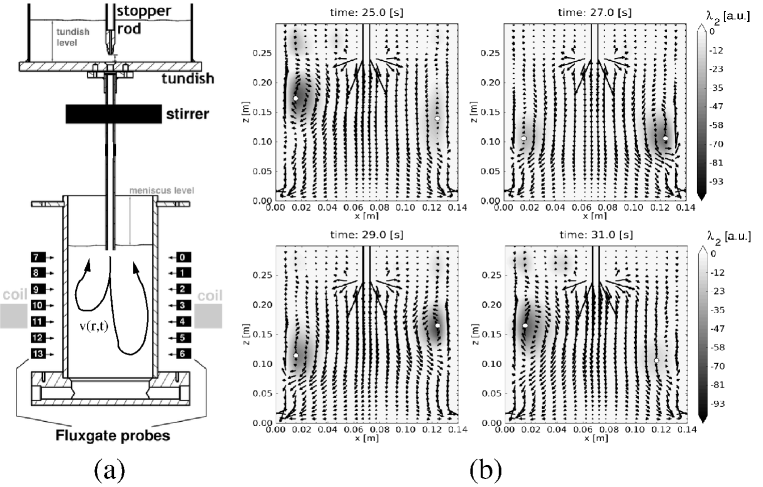
Figure 4: Illustration of the CIFT technique at a model of continuous casting. (a) Experimental set-up with the tundish, the single-port submerged entry nozzle, and the mould. The external field is produced by a coil, and the induced fields are measured at 7 fluxgate sensors at each narrow face of the mould. (b) Four subsequent plots of the velocity field as reconstructed from the measured induced magnetic fields. The quantity $\lambda_{2}$, indicated by the grey scale, is the most appropriate measure for the identification of a vortex (Jeong and Hussain 1995).

5 Conclusions

In this paper we have surveyed the principles and some applications of the integral equation approach (IEA) to kinematic MHD. The IEA has turned out a viable scheme for the correct numerical treatment of dynamo problems in non-spherical domains, for examples in ”matchboxes” and, more importantly, in cylinders (see also Avalos-Zuñiga et al. 2007). It has also proved a good starting point for the treatment of inverse problems of MHD, with direct applications in a number of technical problems characterized by small $R_{m}$.

References

- [1] Avalos-Zuñiga, R., Xu, M., Stefani, F., Gerbeth, G. and Plunian, F., Cylindrical anisotropic dynamos, Geophys. Astrophys. Fluid Dyn., 2007, 101, 389-404.
- [2] Dobler, W. and Rädler, K.-H., Integral equations for kinematic dynamo models. Stud. Geophys. Geod., 1998, 4, 389-404.
- [3] Dobler, W. and Rädler, K.-H., An integral equation approach to kinematic dynamo models. Geophys. Astrophys. Fluid Dyn., 1998, 89, 45-74.
- [4] Gailitis, A., Self-excitation of a magnetic field by a pair of annular vortices. Magnetohydrodynamics, 1970, 6, 14-17.
- [5] Gailitis, A. and Freibergs, Y., Self-excitation of a magnetic field by a pair of annular eddies. Magnetohydrodynamics, 1974, 10, 26-30.
- [6] Gailitis, A. et al., Detection of a flow induced magnetic field eigenmode in the Riga dynamo facility. Phys. Rev. Lett., 2000, 84, 4365-4369.
- [7] Giesecke, A., Stefani, F. and Gerbeth, G., Kinematic simulation of dynamo action by a hybrid boundary-element/finite volume method. Magnetohydrodynamics, 2008, 44, 237-252.
- [8] Giesecke, A., Nore, C., Stefani, F., Gerbeth, G., Léorat, J., Luddens, F., Guermond, J.-L., Electromagnetic induction in non-uniform domains. Geophys. Astrophys. Fluid Dyn., 2010a, 104, 505-529.
- [9] Giesecke, A., Stefani, F. and Gerbeth, G., Role of soft-iron impellers on the mode selection in the von Kármán-sodium dynamo experiment. Phys. Rev. Lett., 2010b, 104, Art. No. 044503.
- [10] Guermond, J.-L., Léorat, J. and Nore, C., A new Finite Element Method for magneto-dynamical problems: two-dimensional results. Eur. J. Mech. B, 2003, 22, 555-579.
- [11] Guermond, J.-L., Laguerre, R., Léorat, J. and Nore, C., An interior penalty Galerkin method for the MHD equations in heterogeneous domains. J. Comp. Phys., 2007, 221, 349-369.
- [12] Guermond, J.-L., Laguerre, R., Léorat, J. and Nore, C., Nonlinear magnetohydrodynamics in axisymmetric heterogeneous domains using a Fourier/finite element technique and an interior penalty method J. Comp. Phys., 2009, 228, 2739-2757.
- [13] Hubbard, A. and Brandenburg, A., Magnetic helicity fluxes in an dynamo embedded in a halo. Geophys. Astrophys. Fluid Dyn., 2010, 104, 577-590.
- [14] Iskakov, A.B., Descombes, S. and Dormy, E., An integro-differential formulation for magnetic induction in bounded domains: boundary element-finite volume method. J. Comp. Phys., 2004, 197, 540-554.
- [15] Iskakov, A.B. and Dormy, E., On magnetic boundary conditions for non-spectral dynamo simulations. Geophys. Astrophys. Fluid Dyn., 2005, 99, 481-492.
- [16] Jeong, J. and Hussain, F., On the identification of a vortex. J. Fluid Mech., 1995, 285, 69-94.
- [17] Krause, F. and Rädler, K.-H., Mean-field Magnetohydrodynamics and Dynamo Theory, 1980 (Berlin: Akademie-Verlag).
- [18] Kenjereš, S., Hanjalić, K., Renaudier, S, Stefani, F, Gerbeth, G and Gailitis, A., Coupled fluid-flow and magnetic-field simulation of the Riga dynamo experiment. Phys. Plasmas, 2006, 13, Art. No. 122308.
- [19] Marie, L., Normand, C. and Daviaud, F., Galerkin analysis of kinematic dynamos in the von Kármán geometry, Phys. Fluids, 2006, 18, Art. No. 017102.
- [20] Monchaux, R. et al., The von Kármán sodium experiment: Turbulent dynamical dynamos. Phys. Fluids, 2009, 21, 035108.
- [21] Nore, C., Léorat, J., Guermond, J.-L. Luddens, F., Nonlinear dynamo action in a precessing cylindrical container. Phys. Rev. E, 2011, 84, Art. No. 016317.
- [22] Rädler, K.-H., Apstein, E., Rheinhardt, M. and Schüler, M., The Karlsruhe dynamo experiment. A mean field approach, Stud. Geophys. Geodaet., 1998, 42, 224-231.
- [23] Rädler, K.-H., Rheinhardt, M., Apstein, E. and Fuchs, H., On the mean-field theory of the Karlsruhe dynamo experiment. Nonlin. Proc. Geophys., 2002, 9, 171-187.
- [24] Roberts, P., An Introduction to Magnetohydrodynamics, 1967 (New York: Elsevier).
- [25] Roberts, P.H. and Scott, S., On the analysis of the secular variation. A hydromagnetic constraint. 1 Theory. J. Geomagn. Geoelectr., 1965, 17, 189-192.
- [26] Stefani, F., Gerbeth, G. and Gailitis, A., Velocity profile optimization for the Riga dynamo experiment. In Transfer Phenomena in Magnetohydrodynamic and electroconducting Flows, edited by A. Alemany, Ph. Marty and J.-P. Thibault, pp. 31-44, 1999 (Kluwer: Dordrecht).
- [27] Stefani, F. and Gerbeth, G., Velocity reconstruction in conducting fluids from magnetic field and electric potential measurements. Inv. Probl., 1999, 15, 771-786.
- [28] Stefani, F. and Gerbeth, G., On the uniqueness of velocity reconstruction in conducting fluids from measurements of induced electromagnetic fields. Inv. Probl., 2000a, 16, 1-9.
- [29] Stefani, F. and Gerbeth, G., A contactless method for velocity reconstruction in electrically conducting fluids. Meas. Sci. Techn., 2000b, 11, 758-765.
- [30] Stefani, F., Gerbeth, G. and Rädler, K.-H., Steady dynamos in finite domains: an integral equation approach. Astron. Nachr., 2000, 321, 65-73.
- [31] Stefani, F. and Gerbeth, G., Oscillatory mean-field dynamos with a spherically symmetric, isotropic helical turbulence parameter . Phys. Rev. E, 2003, 67, Art. No. 027302.
- [32] Stefani, F., Gundrum, T. and Gerbeth, G., Contactless inductive flow tomography. Phys. Rev. E, 2004, 70, Art. No. 056306.
- [33] Stefani, F., Gailitis, A. and Gerbeth, G., Magnetohydrodynamic experiments on cosmic magnetic fields. Zeitschr. Angew. Math. Mech., 2008, 88, 930-954.
- [34] Stefani, F., Gailitis, A. and Gerbeth, G., Numerical simulations of liquid metal experiments on cosmic magnetic fields. Theor. Comp. Fluid Dyn., 2009, 23, 405-429.
- [35] Stieglitz R. and Müller U., Experimental demonstration of the homogeneous two-scale dynamo. Phys. Fluids, 2001, 13, 561-564.
- [36] Wondrak, T., Stefani, F., Gundrum, T, Gerbeth, G, Some methodological improvements of the contactless inductive flow tomography. Int. J. Appl. Electromag. Mech., 2009, 30, 255-264.
- [37] Wondrak, T., Galindo, V., Gerbeth, G., Gundrum, T. Stefani, F. and Timmel, K., Contactless inductive flow tomography for a model of continuous steel casting. Meas. Sci. Techn., 2010, 21, 045402.
- [38] Xu, M., Stefani, F. and Gerbeth, G., The integral equation method for a steady kinematic dynamo problem. J. Comp. Phys., 2004a, 196, 102-125.
- [39] Xu, M., Stefani, F. and Gerbeth, G., Integral equation approach to time-dependent kinematic dynamos in finite domains. Phys. Rev. E, 2004b, 70, Art. No. 056305.
- [40] Xu, M., Stefani, F. and Gerbeth, G., The integral equation approach to kinematic dynamo theory and its application to dynamo experiments in cylindrical geometry. J. Comp. Phys., 2008, 227, 8130-8144.