Soliton driven relaxation dynamics and universality in protein collapse

Abstract

Protein collapse can be viewed as a dynamical phase transition, during which new scales and collective variables become excited while the old ones recede and fade away. This causes formidable computational bottle-necks in approaches that are based on atomic scale scrutiny. Here we consider an effective dynamical Landau theory to model the folding process at biologically relevant time and distance scales. We reach both a substantial decrease in the execution time and improvement in the accuracy of the final configuration, in comparison to more conventional approaches. As an example we inspect the collapse of HP35 chicken villin headpiece subdomain, where there are detailed molecular dynamics simulations to compare with. We start from a structureless, unbend and untwisted initial configuration. In less than one second of wall-clock time on a single processor personal computer we consistently reach the native state with 0.5 Ȧngström root mean square distance (RMSD) precision. We confirm that our folding pathways are indeed akin those obtained in recent atomic level molecular dynamics simulations. We conclude that our approach appears to have the potential for a computationally economical method to accurately understand theoretical aspects of protein collapse.

I Introduction

Structural classification shows that folded proteins in the Protein Data Bank (PDB) pdb are built in a modular fashion from a relatively small number of components comp . In SCOP scop there are presently 1393 unique folds while CATH cath has 1282 different topologies. Both figures have remained unchanged since year 2008. Furthermore, according to xubiao over 90$\%$ of all high resolution PDB proteins can be modeled using no more than 200 explicit soliton motifs as the modular blocks. This convergence in protein architecture proposes that in the vicinity of the native state the atomic level differences between amino acids become less important in determining the fold. Instead the protein shape is dominated collectively, by interactions between a relatively small number of modular components that are made of several amino acids.

Classical molecular dynamics (MD) md -gro remains the only viable approach to describe truly atomic level protein dynamics. With the best available precision MD models very short time and distance scale oscillations of individual atoms, including both their small amplitude thermal fluctuations and the detailed interactions between all the different atoms. But the process of protein folding engages various different temporal and spatial scales. In particular there are several high energy barriers that can be overcome only by relatively slow and collective long range oscillations. These hurdles in scales and structures are the major technical bottle-necks in full atomic level descriptions of protein folding. As a consequence a detailed MD simulation of an entire folding process remains a formidable task. Even in the case of relatively simple and short proteins such as the 35-residue subdomain of the villin headpiece (HP35) where detailed information on the folding dynamics is now becoming available, a detailed simulation can take several months and even years to complete pande -fred2 .

In order to enable practical modeling of the folding, several different effective approaches have been introduced fred2 . Examples range from the coarse-grained Go model and its variants go1 to carefully crafted energy functions such as UNRES sche that explicitely aim to average over those degrees of freedom that are considered to be non-essential for attaining thermodynamically stable structures.

In addition to technical issues, there are also important conceptual matters that need to be addressed in selecting the pertinent coarse grained physical degrees of freedom. In particular, a folding pathway from a structureless straight protein backbone into a biologically active collapsed conformation involves a phase transition. During a phase transition a physical system undergoes a drastic metamorphosis, old factors loose their relevance while new actors enter the stage. In the case of protein folding, the highly localized and short time scale atomic oscillations become replaced by much slower collective motions of extended modular structures. We propose to overcome this dual problem of phases and scales in terms of an effective dynamical Landau-type theory. In analogy of e.g. the effective Landau-Ginzburg theory that models a superconductor in terms of collective Cooper pairs and vortex lines in lieu of the individual electrons and photons of the microscopic BCS theory, we aim to describe the dynamics of protein collapse as a non-conservative Markovian relaxation process of the relevant modular components. In our approach, a protein consistently folds to its PDB structure with a subatomic precision that matches and even exceeds the experimentally determined B-factor Debye-Waller fluctuation distances. Since our description only engages those time and distance scales that characterize biologically relevant motions, we can reach a sub-second execution time of the entire folding process even with an ordinary desktop computer.

II model

The effective Landau energy is oma1 , ulf

$$E=\sum\limits_{i=1}^{N}\biggl{\{}2a\kappa_{i+1}\kappa_{i}+2\kappa_{i}^{2}+b\kappa_{i}^{2}\tau_{i}^{2}+c(\kappa_{i}^{2}-m^{2})\biggr{\}}$$

$$\ +\ \sum\limits_{i=1}^{N}\biggl{\{}d\tau_{i}+q\kappa_{i}^{2}\tau_{i}+e\tau_{i}^{2}\biggr{\}}$$ (1)

Here $\kappa_{i}$ and $\tau_{i}$ are the Frenet bond and torsion angles of the C_α backbone, the summation extends over all backbone angles ($\kappa_{N+1}=0$), see frenet for details. Once these angles are known the protein backbone can be constructed by solving the discrete Frenet equation frenet . The first sum defines the Hamiltonian of the discrete nonlinear Schrödinger equation fadde . In the second sum the first two terms are the conserved helicity and momentum, respectively. The last term is the Proca mass. The functional form (1) is firmly anchored in the elegant mathematical structure of integrable models fadde , it describes the protein backbone in terms of universal physical arguments oma1 . The various parameters have constant values over each of the soliton motifs i.e. they are characteristic only to an entire supersecondary structure such as a helix-loop-helix cherno .

In nora it has been shown that (1) supports solitons as classical solutions. In xubiao it has been shown that over 90$\%$ of all PDB proteins with resolution better than 1.5 Ȧ can be described in a modular fashion in terms of 200 explicitely constructed soliton profiles. The soliton emerges as follows: We first eliminate the variable $\tau_{i}$ in favor of $\kappa_{i}$,

$$\tau_{i}[\kappa_{i}]=-\frac{1}{2}\frac{d+q\,\kappa_{i}^{2}}{e+b\,\kappa_{i}^{2}}$$ (2)

If the value of $\tau_{i}$ falls outside of the fundamental domain $[-\pi,\pi]$ we redefine it modulo $2\pi$. Using the relation (2) and selecting $a=-1.0$ in (1) we then get

$$\kappa_{i+1}-2\kappa_{i}+\kappa_{i-1}\ =\ U^{\prime}[\kappa_{i}]\kappa_{i}\ \equiv\ \frac{dU[\kappa]}{d\kappa_{i}^{2}}\ \kappa_{i}\ \ \ \ (i=1,...,N)$$ (3)

where we define $\kappa_{0}=\kappa_{N+1}=0$. This is a generalization of the DNLS equation with

$$U[\kappa]=-\left(\frac{bd-eq}{2b}\right)^{2}\!\!\cdot\frac{1}{e+b\,\kappa^{2}}-\left(\frac{q^{2}+8bcm^{2}}{4b}\right)\cdot\kappa^{2}+c\cdot\kappa^{4}$$ (4)

With different parameter values its (dark) soliton describes various protein conformations xubiao . But as it stands, the soliton models only static PDB configurations. We now wish to extend this approach into a description of the actual dynamical process of protein folding. Starting from an unbiased initial configuration we aim to reach a soliton arrangement that models the desired static PDB protein with sub-Ȧngström accuracy.

We shall initiate our simulations with a structureless configuration, an unbent and untwisted backbone. This configuration resides in the phase where the radius of gyration scales with Hausdorff dimension $d_{H}=1$. In (1) the parameter $c$ characterizes the average strength of hydrogen bonds along the backbone. The ensuing contribution to energy is largely responsible to the formation of regular secondary structures and the subsequent transition into the collapsed $d_{H}\approx 1/3$ phase. To conform with our initial configuration we start the simulation by setting all $c=0$ initially. During the early stage of the simulation we then introduce the hydrogen bond interactions by swiftly increasing these parameters to their final values, in a uniform manner. At that moment we observe the initial formation of regular secondary structures such as $\alpha$-helices and $\beta$-strands. This is quickly followed by soliton (loop) formation, either by local soliton pair production or by soliton transport throught global deformations. This effectuates a rapid collapse into a molten globule i.e. a configuration in the $d_{H}\approx 1/3$ phase that then proceeds more slowly towards the native state.

As in any phase transition simulation, we need to avoid supercooling that may critically slow down the simulation. For this we utilize the parameter $a$ in (1). Depending on sign, we interpret it as either a ferromagnetic or an antiferromagnetic coupling along a continuous spin Ising chain of the $\kappa_{i}$. The antiferromagnetic order models the folding nuclei that initiate the phase transition, these are essentially the soliton centers. We choose the uniform ferromagnetic coupling $a=-1.0$ for all except those bonds where we foresee the eventual location of the center of a soliton. At the putative soliton locations we introduce an initial repulsive antiferromagnetic coupling with $a=+1.0$. At the first stages of the simulation, in parallel with the introduction of the hydrogen bond interactions, we remove the folding nuclei by decreasing the strength of the antiferromagnetic couplings so that we arrive at the uniform value $a\equiv-1.0$ along the entire backbone. During the entire folding process all other parameters remain intact. With this initial preparation of the hydrogen bond interactions and with the transient introduction of folding nuclei in our otherwise homogeneous backbone, we avoid supercooling into misfolded states with their misplaced or extraneous solitons and soliton-soliton pairs. Even if such states are metastable with an energy (1) that exceeds the energy of the native state and eventually decay, they can have a very long lifetime and substantially slow down the simulations. We remind that in actual proteins the hydrogen bonds are similarly produced during the folding process. There are also natural inhomogeneities in the amino acid structures that act as folding nuclei. Proline is a good example.

We propose that during biologically relevant temporal scales the conformational changes that drive the collapse can be described in terms of an appropriate dynamical universality class. For this we thermally average over all those very short time scale oscillations and tiny fluctuations of individual atoms that are irrelevant to the way how the folding progresses over a biologically relevant time period. The simplest and by far the most natural choice is to utilize a Markovian Monte Carlo time evolution with the standard, universal heat bath probability distribution glauber , lebo

$$\mathcal{P}=\frac{x}{1+x}\ \ \ \ {\rm with}\ \ \ \ x=\exp\{-\frac{\Delta E}{kT}\}$$ (5)

Here $\Delta E$ is the energy difference between consecutive MC time steps that we compute from (1). We choose the numerical value of $kT$ so that we are in the collapsed $d_{H}\approx 1/3$ phase. We have made runs at several different values of $kT$ to confirm that there are no qualitative changes in our results, as long as $d_{H}\approx 1/3$. Since (1) is an approximation of the thermodynamical free energy, the parameters in (1) are a priori temperature dependent and at the moment we (still) lack a direct relation between $kT$ and the physical temperature.

During the time evolution we suffocate any potential rearrangement of covalent bonds along the backbone. For this we introduce a self-avoiding condition ulf that ensures that during the folding process the distance between any two backbone sites remains at least as large as the length of a backbone covalent bond.

We emphasize that (5) does not describe the atomic level details of the folding process. Such details are highly sensitive to the initial configuration including solvent and other environmental factors, to the extent that detailed knowledge of a particular atomic trajectory during the collapse can hardly have any real meaning. Instead the evolution determined by (5) describes the universal statistical aspects of trajectories over biologically relevant scales, how the protein backbone proceeds during the dynamical phase transition from a general class of initial configurations towards its native state.

III example

As an example we consider the folding dynamics of the 35-residue subdomain of the villin headpiece (HP35). The villin is a small ultrafast folding protein that is subject to intense studies by experiments, theory and simulations. The PDB code we use is 1YRF, it describes the crystallographic structure at 95K with 1.07 Ȧ resolution 1yrf . In Table I we list the relevant parameter values in (1) together with the corresponding backbone sites.

parameter	soliton-1	soliton-2
$a$	1.0	1.0
$c_{1}$	0.459712	0.995867
$c_{2}$	4.5533320	9.408796
$m_{1}$	1.504535	1.550322
$m_{2}$	1.512836	1.535081
$b_{\tau}$	- 9.575214e-9	-1.215692e-08
$d_{\tau}$	-6.76965e-11	-7.840467e-08
$e_{\tau}$	2.4378718e-8	2.136684e-08
$q_{\tau}$	6.769649e-10	4.973244e-12
RMSD (Ȧ)	0.38	0.32

Table 1: Parameter values for the two-soliton solution of (2), (3) that describes the backbone of 1YRF with a combined 0.38Ȧ accuracy. The soliton-1 is located between sites 45-57 (PDB indexing) and the soliton-2 is located between PDB sites 58-73. Note that the definition of bond angle $\kappa_{i,i+1}$ takes three and the definition of torsion angle $\tau_{i,i+1}$ takes four sites.

We have determined the parameters by solving (3), (2) to describe the folded structure of 1YRF with an overall 0.38 Ȧ RMSD accuracy.

We start the folding simulation with an initial configuration that is straight line, with all $\kappa_{i,i+1}$ and all $\tau_{i,i+1}$ equal to zero. This is a configuration with Hausdorff dimension $d_{H}=1$, and it minimizes (1) for $c=0$ i.e. when there are no hydrogen bond interactions. We turn on the hydrogen bonds by increasing $c$ to the values in Table I during the first 700.000 steps. We also introduce the folding nuclei by selecting the initial values $a=+1.0$ for two bonds that are located between sites 53-54 and 61-62 corresponding to the centers of the two solitons in 1YRF. We convert these antiferromagnetic couplings into ferromagnetic $a=-1.0$ in tandem with turning on the hydrogen bonds $c$. After this initial preparation we have a random coil configuration. There is a rapid formation of regular secondary structures and a collapse into a molten globule, followed by a relatively slow progress towards the final PDB configuration.

Since we can reach the final configuration in less than one second of total execution time using a single core in a MacPro desktop computer, we are able to collect a large amount of statistical data to investigate the universal aspects of folding pathways. We find that the folding proceeds in a very universal manner, the variations between different runs are very small and the collapse proceeds systematically through steps that are in line with the MD simulation in duan . The collapse starts with the formation of the last helix III. The second loop and the middle helix II then appear, followed by the formation of helix I and the first loop. Towards the end of the collapse the helix I starts to stabilize at a slightly faster rate than the middle helix II. During the final stages the folding process consists mainly from an adjustment of the middle helix II with the two adjacent loops. This helix formation is very similar to the observations made during MD simulations as reported in wallin . This can be seen by comparing our Figure 1 with the corresponding Figure in wallin .

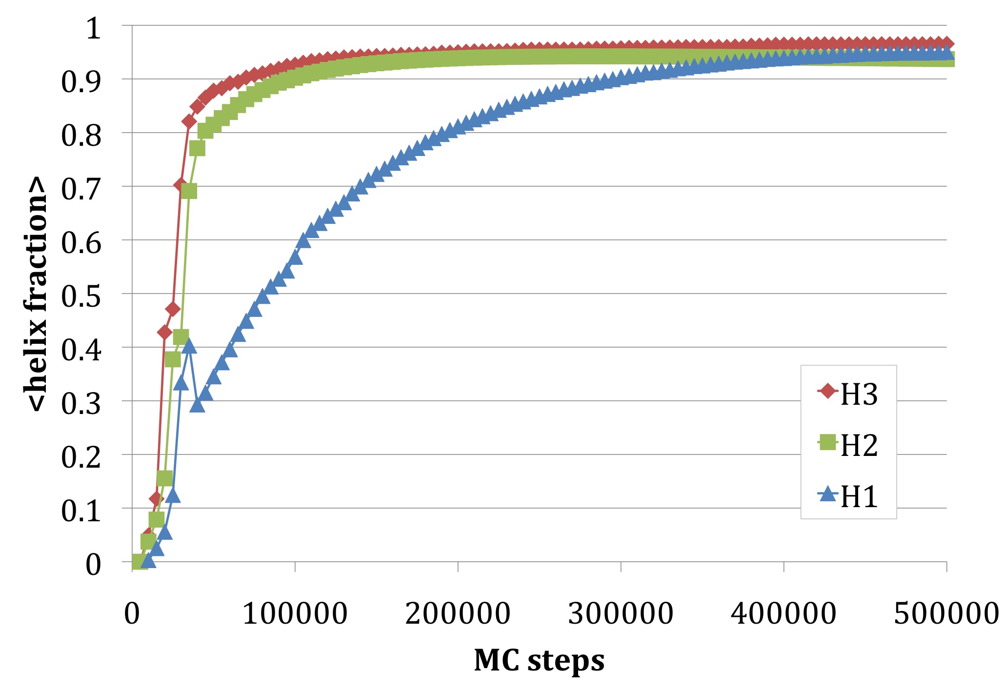
Figure 1: The formation of helices during the collapse of 1YRF, averaged over 4000 trajectories following wallin . The helix II is formed first, and towards the end of the collapse the helix II adjusts itself with the loops.

In Figure 2 we display three generic snap-shot configurations together with the final fold. In a typical simulation we arrive at a structure that deviates from the 1YRF in PDB around 0.5 Ȧngström in RMSD distance. In average, the C_α carbons of the PDB configuration has B-factors that correspond to a Debye-Waller fluctuation distance around 0.4 Ȧ. Consequently we can entirely attribute the average RMSD distance of $\sim 0.5$Ȧ between our final configurations and the PDB structure to thermal fluctuations.

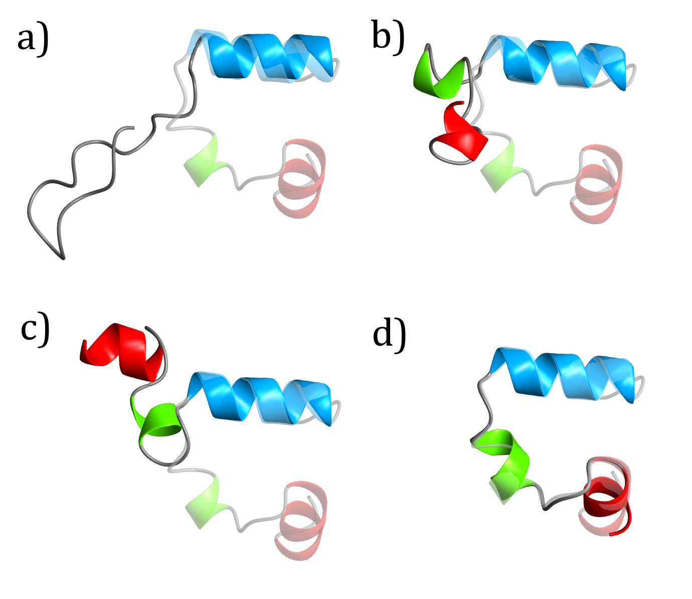
Figure 2: A set of snap-shots of a generic folding pathway in our simulation, over the shadow of the PDB configuration. Color coding shows how the three helices are formed. a) The folding starts with formation of helix III. b) After this, there is formation of the other two helices and loops. c) The folding proceeds with stabilization of middle helix and loops. d) The final fold and the PDB structure of 1YRF generically coincide with RMSD accuracy of about 0.5Ȧ.

IV Discussion

The protein folding problem endures as the pre-eminent unresolved conundrum in science. The major problem in any atomic level simulation relates to time scales and high energy barriers. These can only be overcome with coherent multi-atom collective motions, whose molecular dynamics description remains a formidable task. Here we have introduced a new paradigm for describing and modeling protein collapse. We propose to address the large scale hurdles in terms of solitons in an effective Landau theory and to describe the ensuing collapse dynamics universally, by a non-conservative Markovian heat-bath evolution. We have demonstrated that in the case of 1YRF where MD simulations are available for comparison, the folding pathways obtained in our approach are the same. Among the future challenges is to compute the soliton profiles directly from the individual amino acids, to facilitate predictive collapse simulations.

References

- (1) C Hadley and D.T. Jones, Structure 7 1099 1112 (1999)
- (2) H.M. Berman, K. Henrick, H. Nakamura and J.L. Markley, Nucl. Acids Res. (Database issue) 35 D301-D303 (2007)
- (3) A.G. Murzin, S.E. Brenner, T. Hubbard and C. Chothia, J. Mol. Biol. 247 536-540 (1995)
- (4) L.H. Greene et.al, Nucl. Acids Res. 35 D291-D297 (2007)
- (5) A. Krokhotin, A.J. Niemi and X. Peng, arXiv:1109.3903v1 [physics.bio-ph]
- (6) O.M. Becker, A. Mackerell, B. Roux and M. Watanabe, Comput. Biochem. Biophys. (Marcel Dekker, New York, 2001)
- (7) B.R. Brooks, R.E. Bruccoleri, B.D. Olafson, D.J. States, S. Swaminathan and M. Karplus, J. Comp. Chem. 4 187 217 (1983)
- (8) J.W. Ponder and D.W. Case, Adv. Protein Chem. 66 27 (2003)
- (9) D. van der Spoel, E. Lindahl, B. Hess, G. Groenhof, A.E. Mark and J. Berendsen, Comput. Chem. 26 1701-1718 (2005)
- (10) G. Jayachandran, V. Vishal and V.S. Pande, Journ. Chem. Phys. 124 164902-164912 (2006)
- (11) D.L. Ensign, P.M. Kasson and V.S. Pande, J. Mol. Biol. 374 806-816 (2007)
- (12) H. Lei and Y. Duan, J. Mol. Biol. 370 196-206 (2007)
- (13) J.S. Yang, S. Wallin and E.I. Shakhnovich, PNAS (USA) 105 895-900 (2008)
- (14) P.L. Freddolino and K. Schulten, Biophys. Journ. 97 2338-2347 (2008)
- (15) P.L. Freddolino, C.B. Harrison, Y. Liu and K. Schulten, Nature Phys. 6 751-758 (2010)
- (16) J. Karanicolas J, Brooks, CL III, Protein Sci. 11 2351 2361 (2002)
- (17) A. Liwo, Y. He and A.G. Scheraga, Phys. Chem. Chem. Phys. 13 16890 16901 (2011)
- (18) A.J. Niemi, Phys. Rev. D67 106004-106007 (2003)
- (19) U.H. Danielsson, M. Lundgren and A.J. Niemi, Phys. Rev. E82 021910-021914 (2010)
- (20) S. Hu, M. Lundgren and A.J. Niemi, Phys. Rev. E83 061908-061921 (2011)
- (21) L.D. Faddeev and L.A. Takhtajan, Hamiltonian methods in the theory of solitons (Springer Verlag, Berlin, 1987)
- (22) M. Chernodub, S. Hu and A.J. Niemi, Phys. Rev. E82 011916-011920 (2010)
- (23) N. Molkenthin, S. Hu and A.J. Niemi, Phys. Rev. Lett. 106 078102-078105 (2011)
- (24) R.J. Glauber, Journ. Math. Phys. 4 294-207 (1963)
- (25) A.B. Bortz, M.H. Kalos and J.L. Lebowitz, Journ. Comput. Phys. 17 10-18 (1975)
- (26) M. Chernodub, M. Lundgren and A.J. Niemi, Phys. Rev. E83 011126-011137 (2011)
- (27) T.K. Chiu, J. Kubelka, R. Herbst-Irmer, W.A. Eaton, J. Hofrichter and D.R. Davies, PNAS (USA) 102 7517-7522 (2005)