A Reciprocal Transformation for the Constant Astigmatism Equation

A Reciprocal Transformation
for the Constant Astigmatism Equation

Adam HLAVÁČ and Michal MARVAN

A. Hlaváč and M. Marvan

Mathematical Institute in Opava, Silesian University in Opava,
Na Rybníčku 1, 746 01 Opava, Czech Republic Adam.Hlavac@math.slu.cz, Michal.Marvan@math.slu.cz

Received May 07, 2014, in final form August 14, 2014; Published online August 25, 2014

We introduce a nonlocal transformation to generate exact solutions of the constant astigmatism equation $z_{yy}+(1/z)_{xx}+2=0$. The transformation is related to the special case of the famous Bäcklund transformation of the sine-Gordon equation with the Bäcklund parameter $\lambda=\pm 1$. It is also a nonlocal symmetry.

constant astigmatism equation; exact solution; constant astigmatism surface; orthogonal equiareal pattern; reciprocal transformation; sine-Gordon equation

53A05; 35A30; 35C05; 37K35

1 Introduction

In this paper, we continue investigation of the constant astigmatism equation

$$z_{yy}+\left(\frac{1}{z}\right)_{xx}+2=0,$$ (1)

which is the Gauss equation for constant astigmatism surfaces immersed in the Euclidean space; see [2]. These surfaces are defined by the condition $\sigma-\rho={\rm const}$, where $\rho$, $\sigma$ are the principal radii of curvature and the constant is nonzero. Without loss of generality, the ambient space may be scaled so that the constant is $\pm 1$, which is assumed in what follows. The same equation (1) describes spherical orthogonal equiareal patterns; see later in this section.

A brief history of constant astigmatism surfaces is included in [2, 23] (apparently, they had no name until [2]). Ribaucour [24] and Bianchi [4, 6] observed that evolutes (focal surfaces) of constant astigmatism surfaces are pseudospherical (of constant negative Gaussian curvature). Conversely, involutes of pseudospherical surfaces corresponding to parabolic geodesic nets are of constant astigmatism. This yields a pair of nonlocal transformations [2] between the constant astigmatism equation (1) and the integrable sine-Gordon equation

$$u_{\alpha\beta}=\sin u,$$ (2)

which is the Gauss equation for pseudospherical surfaces in terms of asymptotic Chebyshev coordinates $\alpha$, $\beta$. Hence, the constant astigmatism equation is also integrable; see [2] for its zero curvature representation. Moreover, the famous Bianchi superposition principle for the sine-Gordon equation can be extended in such a way that an arbitrary number of solutions of the constant astigmatism equation can be obtained by purely algebraic manipulations and differentiation; see [13].

The class of sine-Gordon solutions that can serve as a seed is limited, since the initial step involves integration of the nonlinear (although linearisable) equations (23) below. The class contains all multisoliton solutions, which themselves can be generated from the zero seed. Another successfully planted seed we know of is the travelling wave used by Hoenselaers and Miccichè [15].

In this paper, we look for another solution-generating tool that would not require solving differential equations. We introduce two (interrelated) auto-transformations $\mathcal{X}_{A}$ and $\mathcal{Y}_{B}$ that, in geometric terms, correspond to taking the involute of the evolute. Each generates a three-parametric family of solutions from a single seed, but when applied in combination, they have an unlimited generating power in terms of the number of arbitrary parameters in the solution.

The transformations $\mathcal{X}_{A}$ and $\mathcal{Y}_{B}$ are Bäcklund transformations sensu Bäcklund [1, 12], since each is determined by four relations of no more than the first order (although modern usage often sees this term as implying that independent variables are preserved, the original meaning is as stated). We call $\mathcal{X}_{A}$ and $\mathcal{Y}_{B}$ reciprocal transformations since, up to point transformations, $\mathcal{X}_{A}$ and $\mathcal{Y}_{B}$ are equivalent to $\mathcal{X}$ and $\mathcal{Y}$ satisfying

$$\mathcal{X}^{2}=\mathcal{Y}^{2}={\rm Id},$$

which is a property characteristic of reciprocal transformations [16]. For the history and overview of reciprocal transformations and their wide applications in physics and geometry see [27, Chapter 3] and [25, Section 6.4]. Reciprocal invariants, linked to invariants in Lie sphere geometry, are available in the context of hydrodynamic-type systems [8, 9, 10]. Geometry of immersed surfaces is rich in nonlocal transformations to the sine-Gordon equation, see, e.g., [26, § 3.3]; this example is of particular interest in the context of our present efforts (compare [26, equation (3.27)] to [3, Table 1, row 6b]). Nonlocal transformations between general integrable equations are often reciprocal or decomposable into a chain where one of the factors is reciprocal; this extends to hierarchies, see [28] and [26, § 6.4].

Transformations $\mathcal{X}_{A}$ and $\mathcal{Y}_{B}$ only depend on the computation of path-independent line integrals, which puts lower demands on the seeds. The sine-Gordon equation is bypassed and the transformations are immediately applicable to solutions of the constant astigmatism equation with no apriori given sine-Gordon counterpart, such as the Lipschitz solution [14, 18]. If the seeds are given in parametric form, then so are the generated solutions.

Our work would be incomplete without explicitly constructing the transformed surface of constant astigmatism. To obtain compact formulas, a small but useful digression is made. According to [13], to every surface of constant astigmatism there corresponds an orthogonal equiareal pattern on the Gaussian sphere; the same conclusion was made by Bianchi [6, § 375, equation (20)] in the context of pseudospherical congruences. By an orthogonal equiareal pattern [13, 29, 30] we mean a parameterization such that the metric assumes the form

$$z\,{\mathrm{d}}x^{2}+\frac{1}{z}\,{\mathrm{d}}y^{2}$$

(which is, incidentally, of relevance to two-dimensional plasticity under the Tresca yield condition, [29]). The name reflects the fact that “uniformly spaced” coordinate lines $x=a_{1}t+a_{0}$ and $y=b_{1}s+b_{0}$, where $a_{1},a_{0},b_{1},b_{0}={\rm const}$, form equiareal curvilinear rectangles.

The contents of this paper are as follows. In Section 2 we recall symmetries and conservation laws of the constant astigmatism equation. Section 3 contains a derivation of the reciprocal transformations. Starting with a constant astigmatism surface we construct its pseudospherical evolute and then a family of new parallel surfaces of constant astigmatism. New solutions of the constant astigmatism equation then result from finding curvature coordinates on these surfaces. Section 4 summarizes the transformations obtained in the preceding section. In Section 5 we obtain the same transformations as nonlocal symmetries of the constant astigmatism equation. In Section 6 we show that they correspond to the Bäcklund transformation for the sine-Gordon equation with the Bäcklund parameter $\lambda=\pm 1$. In Section 7 we describe the transformations in terms of the constant astigmatism surfaces and the orthogonal equiareal patterns on the Gaussian sphere. Finally, the last section contains several exact solutions.

2 Point symmetries

According to [2], there are three independent continuous Lie symmetries of equation (1): the $x$-translation

$${\mathcal{T}}^{x}_{a}(x,y,z)=(x+a,y,z),\qquad a\in{\mathbb{R}},$$

the $y$-translation

$${\mathcal{T}}^{y}_{b}(x,y,z)=(x,y+b,z),\qquad b\in{\mathbb{R}},$$

and the scaling

$${\mathcal{S}}_{c}(x,y,z)=\big{(}x/c,cy,c^{2}z\big{)},\qquad c\in{\mathbb{R}}\setminus\{0\}.$$

The known discrete symmetries are exhausted by the involution (or duality)

$${\mathcal{J}}(x,y,z)=\left(y,x,\frac{1}{z}\right),$$

the $x$-reversal ${\mathcal{R}}^{x}(x,y,z)=(-x,y,z)$, and the $y$-reversal ${\mathcal{R}}^{y}(x,y,z)=(x,-y,z)$. To avoid possible misunderstanding, we stress that ${\mathcal{T}}^{x}$, ${\mathcal{T}}^{y}$, ${\mathcal{R}}^{x}$, ${\mathcal{R}}^{y}$ should be understood as single symbols, similarly to ${\mathcal{S}}$, ${\mathcal{J}}$. The superscripts $x$, $y$ refer to the affected position in the triple $(x,y,z)$.

Obviously,

$${\mathcal{J}}\circ{\mathcal{J}}={\rm Id},\qquad {\mathcal{J}}\circ{\mathcal{T}}^{x}_{a}={\mathcal{T}}^{y}_{a}\circ{\mathcal{J}},\qquad {\mathcal{J}}\circ{\mathcal{T}}^{y}_{a}={\mathcal{T}}^{x}_{a}\circ{\mathcal{J}},$$

$${\mathcal{S}}_{c}\circ{\mathcal{T}}^{x}_{a}={\mathcal{T}}^{x}_{a/c}\circ{\mathcal{S}}_{c},\qquad {\mathcal{S}}_{c}\circ{\mathcal{T}}^{y}_{b}={\mathcal{T}}^{y}_{cb}\circ{\mathcal{S}}_{c},\qquad {\mathcal{S}}_{c}\circ{\mathcal{J}}={\mathcal{J}}\circ{\mathcal{S}}_{1/c},\qquad {\mathcal{R}}^{x}\circ{\mathcal{S}}_{-1}={\mathcal{R}}^{y}.$$

Translations and reversals correspond to mere reparameterizations of the constant astigmatism surfaces. The scaling symmetry takes a surface to a parallel surface, obtained when moving every point of the surface a constant distance along the normal (offsetting). The involution swaps the orientation, interchanges $x$ and $y$, and makes a unit offsetting. Solutions invariant with respect to the local Lie symmetries can be found in [14, Proposition 1]; they correspond to the Lipschitz [18] class of constant astigmatism surfaces. Higher order symmetries have been considered in [2] and [21]; they will not be needed in this paper.

We shall also need the six first-order conservation laws of equation (1), which are easy to compute following, e.g., [7]. The associated six potentials $\chi$, $\eta$, $\xi$, $\theta$, $\alpha$, $\beta$ satisfy

$$\chi_{x}=z_{y}+y,\qquad \chi_{y}=\frac{z_{x}}{z^{2}}-x,$$

$$\eta_{x}=xz_{y},\qquad \eta_{y}=x\frac{z_{x}}{z^{2}}+\frac{1}{z}-x^{2},$$

$$\xi_{x}=-yz_{y}+z-y^{2},\qquad \xi_{y}=-y\frac{z_{x}}{z^{2}},$$

$$\theta_{x}=xyz_{y}-xz+\frac{1}{2}xy^{2},\qquad \theta_{y}=xy\frac{z_{x}}{z^{2}}+\frac{y}{z}-\frac{1}{2}x^{2}y$$ (3)

and

$$\alpha_{x}=\frac{\sqrt{(z_{x}+zz_{y})^{2}+4z^{3}}}{4z},\qquad \alpha_{y}=\frac{\sqrt{(z_{x}+zz_{y})^{2}+4z^{3}}}{4z^{2}},$$

$$\beta_{x}=\frac{\sqrt{(z_{x}-zz_{y})^{2}+4z^{3}}}{4z},\qquad \beta_{y}=-\frac{\sqrt{(z_{x}-zz_{y})^{2}+4z^{3}}}{4z^{2}}.$$ (4)

Equations (3), (4) are compatible by virtue of equation (1). It is not a pure coincidence that the same symbols $\alpha$, $\beta$ occur in equations (2) and (4), see Section 6 below. Assuming $z$ positive in accordance to its geometrical meaning [2, 13], the radicands in (4) are positive as well. On the other hand, Manganaro and Pavlov [19] considered the class of solutions such that one of the two radicands is zero.

The involution ${\mathcal{J}}$ acts on the potentials as follows: $\eta\leftrightarrow\xi$, while $\chi\to-\chi$, $\theta\to-\theta$, $\alpha\leftrightarrow\alpha$, and $\beta\leftrightarrow-\beta$. The action of the other symmetries is considered below.

3 A geometric construction

Let $z(x,y)$ be a solution of the constant astigmatism equation (1). Under the choice of scale such that $\sigma-\rho=1$, the fundamental forms of the corresponding surface of constant astigmatism are

$$\mathbf{I}=u^{2}\,{\mathrm{d}}x^{2}+v^{2}\,{\mathrm{d}}y^{2},\qquad\mathbf{II}=\frac{u^{2}}{\rho}\,{\mathrm{d}}x^{2}+\frac{v^{2}}{\sigma}\,{\mathrm{d}}y^{2},$$

where

$$u=\frac{\ln z-2}{2}\sqrt{z},\qquad v=\frac{\ln z}{2\sqrt{z}},\qquad\rho=\frac{\ln z-2}{2},\qquad\sigma=\frac{\ln z}{2},\qquad$$

see [3]. Obviously,

$$uv=\rho\sigma.$$ (5)

Once $\sigma-\rho=\pm 1$, equation (5) means that $x$, $y$ are the adapted curvature coordinates in the sense of [13, Definition 1] (they are also normal coordinates in the sense of [11]).

The corresponding surface $\mathbf{r}(x,y)$ of constant astigmatism and its unit normal $\mathbf{n}(x,y)$ satisfy the Gauss–Weingarten system

$$\mathbf{r}_{xx}=\frac{(\ln z)z_{x}}{2(\ln z-2)z}\mathbf{r}_{x}-\frac{(\ln z-2)zz_{y}}{2\ln z}\mathbf{r}_{y}+\frac{1}{2}(\ln z-2)z\mathbf{n},$$

$$\mathbf{r}_{xy}=\frac{(\ln z)z_{y}}{2(\ln z-2)z}\mathbf{r}_{x}-\frac{(\ln z-2)z_{x}}{2z\ln z}\mathbf{r}_{y},$$

$$\mathbf{r}_{yy}=\frac{(\ln z)z_{x}}{2(\ln z-2)z^{3}}\mathbf{r}_{x}-\frac{(\ln z-2)z_{y}}{2z\ln z}\mathbf{r}_{y}+\frac{\ln z}{2z}\mathbf{n},$$

$$\mathbf{n}_{x}=-\frac{2}{\ln z-2}\mathbf{r}_{x},\qquad\mathbf{n}_{y}=-\frac{2}{\ln z}\mathbf{r}_{y},$$ (6)

which is compatible as a consequence of equation (1).

Let us construct the pseudospherical evolute [4] of the surface $\mathbf{r}$. By definition, the evolute has two sheets formed by the loci of the principal centres of curvature. We choose one of the two evolutes, given by

$$\hat{\mathbf{r}}=\mathbf{r}+\sigma\mathbf{n},\qquad\hat{\mathbf{n}}=\frac{\mathbf{r}_{y}}{v}=\frac{2\sqrt{z}}{\ln z}\mathbf{r}_{y}.$$

The first fundamental form of this evolute is

$$\hat{\mathbf{I}}=\frac{4{z}^{3}+z_{x}^{2}}{4{z}^{2}}\,{\mathrm{d}}x^{2}+\frac{z_{x}z_{y}}{2{z}^{2}}\,{\mathrm{d}}x\,{\mathrm{d}}y+\frac{z_{y}^{2}}{4{z}^{2}}\,{\mathrm{d}}y^{2}=z\,{\mathrm{d}}x^{2}+\frac{{\mathrm{d}}z^{2}}{4z^{2}}.$$

One easily sees that the Gauss curvature is $-1$, as expected.

Next we construct the involute to this pseudospherical surface in order to obtain a new surface of constant astigmatism together with a new solution of the equation (1). Following [5, § 136] (see also [31]), we let $X$ and $Y$ be parabolic geodesic coordinates on the pseudospherical surface. By definition, the first fundamental form should be

$$\hat{\mathbf{I}}={\mathrm{d}}X^{2}+{\mathrm{e}}^{2X}{\mathrm{d}}Y^{2}.$$

Comparing the coefficients, we obtain

$$X_{x}^{2}+{\mathrm{e}}^{2X}Y_{x}^{2}=z+\frac{z_{x}^{2}}{4z^{2}},\qquad 2X_{x}X_{y}+2{\mathrm{e}}^{2X}Y_{x}Y_{y}=\frac{z_{x}z_{y}}{2z^{2}},\qquad X_{y}^{2}+{\mathrm{e}}^{2X}Y_{y}^{2}=\frac{z_{y}^{2}}{4z^{2}}.$$

Solving the last two equations for $Y_{x}$, $Y_{y}$, we have

$$Y_{x}=\frac{z_{x}z_{y}-4z^{2}X_{x}X_{y}}{2z{\mathrm{e}}^{X}\sqrt{\smash{z_{y}^{2}-4z^{2}X_{y}^{2}}\hbox{\vrule width=0.0pt,height=8.61108pt,depth=1.29167pt}}},\qquad Y_{y}=\frac{\sqrt{\smash{z_{y}^{2}-4z^{2}X_{y}^{2}}\hbox{\vrule width=0.0pt,height=8.61108pt,depth=1.29167pt}}\hbox{\vrule width=0.0pt,height=8.61108pt,depth=4.30554pt}}{2z{\mathrm{e}}^{X}},$$ (7)

which allows us to convert the remaining equation into

$$X_{x}=\frac{z_{x}X_{y}+\sqrt{\smash{zz_{y}^{2}-4z^{3}X_{y}^{2}}\hbox{\vrule width=0.0pt,height=8.61108pt,depth=1.29167pt}}\hbox{\vrule width=0.0pt,height=8.61108pt,depth=4.30554pt}}{z_{y}}.$$ (8)

Substituting into (7) and performing cross-differentiation, we obtain

$$X_{yy}=-X_{y}^{2}+\frac{zz_{xx}-2z_{x}^{2}-z^{2}z_{y}^{2}-2z^{3}}{z^{3}z_{y}}X_{y}+\frac{z_{y}^{2}}{4z^{2}}.$$ (9)

Now the system consisting of equations (7), (8) and (9) is compatible by virtue of equation (1).

The involute we look for is given by

$$\tilde{\mathbf{r}}=\hat{\mathbf{r}}+(a-X)\hat{\mathbf{r}}_{X}=\mathbf{r}+\left(\frac{1}{2}\ln z+{\frac{2z(a-X)X_{y}}{z_{y}}}\right)\mathbf{n}+2(a-X)\frac{\sqrt{\smash{z_{y}^{2}-4{z}^{2}X_{y}^{2}}\hbox{\vrule width=0.0pt,height=8.61108pt,depth=1.29167pt}}\hbox{\vrule width=0.0pt,height=8.61108pt,depth=4.30554pt}}{\sqrt{z}z_{y}(2-\ln z)}\mathbf{r}_{x},$$ (10)

where $a$ is an arbitrary constant. The unit normal vector to the involute is

$$\tilde{\mathbf{n}}=\hat{\mathbf{r}}_{X}=\frac{2zX_{y}}{z_{y}}\mathbf{n}-\frac{2\sqrt{\smash{z_{y}^{2}-4{z}^{2}X_{y}^{2}}\hbox{\vrule width=0.0pt,height=8.61108pt,depth=1.29167pt}}\hbox{\vrule width=0.0pt,height=8.61108pt,depth=4.30554pt}}{\sqrt{z}z_{y}(\ln z-2)}\mathbf{r}_{x}.$$

To obtain $X$, we have to solve the compatible system (8), (9). The other unknown $Y$ is no more needed.

The system (8), (9) has the obvious particular solution

$$X_{0}=\tfrac{1}{2}\ln z+c_{2},$$

which corresponds to the constant astigmatism surface $\tilde{\mathbf{r}}=\mathbf{r}+(a-c_{2})\mathbf{n}$. Thus, we recover the constant astigmatism surface we started with along with all its parallel surfaces.

To find the general solution of the system (8), (9), we first observe that (9) is a Riccati equation in $X_{y}$. Knowing one particular solution $X_{0,y}$ is sufficient for finding the general solution $X_{y}$, see, e.g., [22]. Omitting the details, we present the general solution

$$X=\ln\frac{(x+c_{1})^{2}z+1}{\sqrt{z}}+c_{2}$$ (11)

of the system (8), (9). In order to simplify the formulas below, we remove the integration constant $c_{1}$ by reparameterization ${\mathcal{T}}^{x}_{c_{1}}$. Then

$$X=\ln\frac{x^{2}z+1}{\sqrt{z}}+c_{2},$$

which, if substituted into formula (10), yields the family of involutes

$$\tilde{\mathbf{r}}=\mathbf{r}+\left(\frac{x^{2}z\ln z}{x^{2}z+1}+\frac{x^{2}z-1}{x^{2}z+1}\big{(}\ln\big{(}x^{2}z+1\big{)}+a\big{)}\right)\mathbf{n}+2x\frac{2a-2\ln\big{(}x^{2}z+1\big{)}+\ln z}{\big{(}x^{2}z+1\big{)}(2-\ln z)}\mathbf{r}_{x},$$ (12)

where $c_{2}$ has been absorbed into $a$. The corresponding unit normal is

$$\tilde{\mathbf{n}}=\frac{x^{2}z-1}{x^{2}z+1}\mathbf{n}+\frac{4x}{\big{(}x^{2}z+1\big{)}(2-\ln z)}\mathbf{r}_{x}.$$ (13)

A routine computation (see below) shows that the surface $\tilde{\mathbf{r}}(x,y)$ has a constant astigmatism, and so has $\tilde{\mathbf{r}}(x+c_{1},y)$, which corresponds to $X$ given by the general solution (11). The parameter $a$ corresponds to the offsetting, meaning a parallel surface.

However, one more step is required in order to find the corresponding solution of equation (1). Namely, we have to find the adapted curvature coordinates $x^{\prime}$, $y^{\prime}$ for the involute. In order that $x^{\prime}$, $y^{\prime}$ be curvature coordinates, $\partial/\partial x^{\prime}$ and $\partial/\partial y^{\prime}$ have to be eigenvectors of the shape operator. The shape operator is too lengthy to be written here, but its eigenvalues (principal curvatures) $1/\rho^{\prime}$, $1/\sigma^{\prime}$ are simple enough (cf. equation (15) below). Computing the eigenvectors, and choosing an assignment between $\partial/\partial x^{\prime}$, $\partial/\partial y^{\prime}$ and the two eigenvectors, we obtain

$$x^{\prime}_{y}=\frac{xz_{y}}{xz_{x}-x^{2}z^{2}+z}x^{\prime}_{x},\qquad y^{\prime}_{y}=\frac{xz_{x}-x^{2}z^{2}+z}{xz^{2}z_{y}}y^{\prime}_{x}.$$ (14)

Under conditions (14), we have

$$\tilde{\mathbf{I}}=u^{\prime 2}\,{\mathrm{d}}x^{\prime 2}+v^{\prime 2}\,{\mathrm{d}}y^{\prime 2},\qquad\tilde{\mathbf{II}}=\frac{u^{\prime 2}}{\rho^{\prime}}\,{\mathrm{d}}x^{\prime 2}+\frac{v^{\prime 2}}{\sigma^{\prime}}\,{\mathrm{d}}y^{\prime 2},$$

where

$$\rho^{\prime}=\ln\frac{\sqrt{z}}{x^{2}z+1}+a+1,\qquad \sigma^{\prime}=\ln\frac{\sqrt{z}}{x^{2}z+1}+a,$$

$$u^{\prime}=\frac{xz_{x}-x^{2}z^{2}+z}{(x^{2}z+1)\sqrt{z}}\frac{\rho^{\prime}}{x^{\prime}_{x}},\qquad v^{\prime}=\frac{x\sqrt{z}z_{y}}{x^{2}z+1}\frac{\sigma^{\prime}}{y^{\prime}_{x}}.$$ (15)

We immediately see that $\rho^{\prime}-\sigma^{\prime}=1$, which implies that the surface $\tilde{\mathbf{r}}$ is of constant astigmatism as required.

In order that $x^{\prime}$, $y^{\prime}$ be adapted in the sense of [13, Definition 1], we require $u^{\prime}v^{\prime}=\pm\rho^{\prime}\sigma^{\prime}$, which implies

$$y^{\prime}_{x}=\pm\frac{xz_{x}-x^{2}z^{2}+z}{\big{(}x^{2}z+1\big{)}^{2}}\frac{xz_{y}}{x^{\prime}_{x}}.$$ (16)

The second equation (14) becomes

$$y^{\prime}_{y}=\pm\left(\frac{xz_{x}-x^{2}z^{2}+z}{\big{(}x^{2}z+1\big{)}z}\right)^{2}\frac{1}{x^{\prime}_{x}}.$$ (17)

By cross-differentiation between equations (16) and (17), we obtain the second-order equation

$$x^{\prime}_{xx}=\frac{x\big{(}x^{2}z+1\big{)}z_{xx}-2x^{3}z_{x}^{2}-6x^{2}zz_{x}+2z_{x}+2x^{3}z^{3}-6xz^{2}}{\big{(}x^{2}z+1\big{)}\big{(}xz_{x}-x^{2}z^{2}+z\big{)}}x^{\prime}_{x},$$

possessing the general solution

$$x^{\prime}_{x}=b\frac{xz_{x}-x^{2}z^{2}+z}{\big{(}x^{2}z+1\big{)}^{2}},$$

where $b$ denotes an arbitrary function of $y$. Inserting into (14), (16) and (17), we obtain

$$x^{\prime}_{y}=b\frac{xz_{y}}{(x^{2}z+1)^{2}},\qquad y^{\prime}_{x}=\pm\frac{1}{b}xz_{y},\qquad y^{\prime}_{y}=\pm\frac{1}{b}\frac{xz_{x}-x^{2}z^{2}+z}{z^{2}}.$$

By cross-differentiation between the two equations on $y^{\prime}$, we receive $b_{y}=0$, meaning that $b$ is a constant. The last four equations on $x^{\prime}$ and $y^{\prime}$ are compatible now; their general solution is simply

$$x^{\prime}=b\frac{xz}{x^{2}z+1}+c_{2},\qquad y^{\prime}=\pm\frac{1}{b}\eta+c_{3},$$

where

$${\mathrm{d}}\eta=xz_{y}\,{\mathrm{d}}x+\left(x\frac{z_{x}}{z^{2}}+\frac{1}{z}-x^{2}\right){\mathrm{d}}y$$

as introduced in Section 2 above. Finally,

$$\tilde{\mathbf{III}}=\frac{1}{b^{2}}\frac{\big{(}x^{2}z+1\big{)}^{2}}{z}\,{\mathrm{d}}x^{\prime 2}+b^{2}\frac{z}{\big{(}x^{2}z+1\big{)}^{2}}\,{\mathrm{d}}y^{\prime 2}.$$

Hence,

$$z^{\prime}=\frac{1}{b^{2}}\frac{\big{(}x^{2}z+1\big{)}^{2}}{z}.$$

Recall that we applied the translation ${\mathcal{T}}^{x}_{c_{1}}$ after equation (11) in order to remove the parameter $c_{1}$. Reintroducing $c_{1}$, which amounts to replacing $x$ with $x+c_{1}$ in the above formulas, we obtain

$$x^{\prime}=b\frac{(x+c_{1})z}{(x+c_{1})^{2}z+1}+c_{2},\qquad y^{\prime}=\pm\frac{1}{b}\big{(}\eta+c_{1}\chi-c_{1}xy-c_{1}^{2}y\big{)}+c_{3},$$

$$z^{\prime}=\frac{1}{b^{2}}\frac{((x+c_{1})^{2}z+1)^{2}}{z},$$ (18)

where $\chi$ was introduced in Section 2 above. The parameters $c_{i}$ can be conveniently encoded in a matrix, see Proposition 4.7 below.

To sum up, we started with a constant astigmatism surface $\mathbf{r}$, constructed its pseudospherical image $\hat{\mathbf{r}}$, then reconstructed the full preimage $\tilde{\mathbf{r}}$, reflecting the freedom of choice of the parabolic geodesic system on $\hat{\mathbf{r}}$. Accordingly, it should not come as a surprise that the transformation has a limited generating power, measured by the number of arbitrary constants the resulting solution depends on. The generating power becomes unlimited only if two such transformations, using different sheets of the evolute, are combined. This will be discussed in Section 6 below.

4 The reciprocal transformations and their properties

Consider the formulas (18). Setting all integration constants $c_{i}$ to zero, $b$ to $1$, and choosing the ‘$+$’ sign, we obtain a transformation $\mathcal{X}(x,y,z)=(x^{\prime},y^{\prime},z^{\prime})$, defined by

$$x^{\prime}=\frac{xz}{x^{2}z+1},\qquad y^{\prime}=\eta,\qquad z^{\prime}=\frac{\big{(}x^{2}z+1\big{)}^{2}}{z}.$$ (19)

Using conjugation with the involution ${\mathcal{J}}$, we obtain another transformation $\mathcal{Y}(x,y,z)=(x^{*}$, $y^{*},z^{*})$, where

$$x^{*}=\xi,\qquad y^{*}=\frac{y}{y^{2}+z},\qquad z^{*}=\frac{z}{\big{(}y^{2}+z\big{)}^{2}}.$$ (20)

Formulas (20) follow from formulas (19) and the relation ${\mathcal{Y}}={\mathcal{J}}\circ{\mathcal{X}}\circ{\mathcal{J}}$.

Remark 4.1.

We remind the reader that $\xi$ and $\eta$ are potentials defined in Section 2. Therefore, they are unique up to an integration constant, which is not to be neglected, because it represents a parameter in the solution. Alternatively speaking, symbols ${\mathcal{X}}$ and ${\mathcal{Y}}$ can be viewed as standing for the compositions ${\mathcal{T}}^{y}_{b}\circ{\mathcal{X}}$ and ${\mathcal{T}}^{x}_{a}\circ{\mathcal{Y}}$, respectively, where $a,b$ are arbitrary constants.

Proposition 4.2.

Let $z(x,y)$ be a solution of the constant astigmatism equation (1), $\xi$, $\eta$ the corresponding potentials (3). Let ${\mathcal{X}}(x,y,z)=(x^{\prime},y^{\prime},z^{\prime})$ and ${\mathcal{Y}}(x,y,z)=(x^{*},y^{*},z^{*})$ be determined by formulas (19) and (20). Then $z^{\prime}(x^{\prime},y^{\prime})$ and $z^{*}(x^{*},y^{*})$ are solutions of the constant astigmatism equation (1) as well.

Proof 4.3.

The statement follows from the reasoning in the preceding section. A routine, straightforward, but cumbersome proof consists in computing $z^{\prime}_{x^{\prime}x^{\prime}}+(1/z^{\prime})_{y^{\prime}y^{\prime}}+2=0$.

Let us note that the first derivatives transform according to the formulas

$$\left(\begin{matrix}z^{\prime}_{x^{\prime}}\\ z^{\prime}_{y^{\prime}}\end{matrix}\right)=J_{{\mathcal{X}}}^{-1}\left(\begin{matrix}z^{\prime}_{x}\\ z^{\prime}_{y}\end{matrix}\right),\qquad\left(\begin{matrix}z^{*}_{x^{*}}\\ z^{*}_{y^{*}}\end{matrix}\right)=J_{{\mathcal{Y}}}^{-1}\left(\begin{matrix}z^{*}_{x}\\ z^{*}_{y}\end{matrix}\right),$$

where $J_{{\mathcal{X}}}$ and $J_{{\mathcal{Y}}}$ are the Jacobi matrices

$$J_{{\mathcal{X}}}=\left(\begin{matrix}x^{\prime}_{x}&y^{\prime}_{x}\\ x^{\prime}_{y}&y^{\prime}_{y}\end{matrix}\right)=\left(\begin{matrix}\dfrac{xz_{x}-x^{2}z^{2}+z}{\big{(}x^{2}z+1\big{)}^{2}}&xz_{y}\vspace{1mm}\\ \dfrac{xz_{y}}{\big{(}x^{2}z+1\big{)}^{2}}&\dfrac{xz_{x}-x^{2}z^{2}+z}{z^{2}}\end{matrix}\right),$$

$$J_{{\mathcal{Y}}}=\left(\begin{matrix}x^{*}_{x}&y^{*}_{x}\\ x^{*}_{y}&y^{*}_{y}\end{matrix}\right)=\left(\begin{matrix}-yz_{y}+z-y^{2}&-\dfrac{yz_{x}}{\big{(}z+y^{2}\big{)}^{2}}\vspace{1mm}\\ -\dfrac{yz_{x}}{z^{2}}&-\dfrac{yz_{y}-z+y^{2}}{\big{(}z+y^{2}\big{)}^{2}}\end{matrix}\right).$$

Formulas for the second derivatives are too lengthy to be printed.

Proposition 4.4.

Under a suitable choice of integration constants, ${\mathcal{X}}\circ{\mathcal{X}}={\rm Id}$ and ${\mathcal{Y}}\circ{\mathcal{Y}}={\rm Id}$.

Proof 4.5.

It is straightforward to see that $x^{\prime\prime}=x^{\prime}z^{\prime}/(x^{\prime 2}z^{\prime}+1)=x$ and $z^{\prime\prime}=(x^{\prime 2}z^{\prime}+1)^{2}/z^{\prime}=z$. Let us compute $y^{\prime\prime}=\eta^{\prime}$, omitting technical details. According to (3), $\eta^{\prime}$ is defined by

$$\eta^{\prime}_{x^{\prime}}=x^{\prime}z^{\prime}_{y^{\prime}}=-\frac{(x^{2}z+1)^{2}xz^{2}z_{y}}{\big{(}xz_{x}-x^{2}z^{2}+z+xzz_{y}\big{)}\big{(}xz_{x}-x^{2}z^{2}+z-xzz_{y}\big{)}},$$

$$\eta^{\prime}_{y^{\prime}}=x^{\prime}\frac{z^{\prime}_{x^{\prime}}}{z^{\prime 2}}+\frac{1}{z^{\prime}}-x^{\prime 2}=\frac{\big{(}xz_{x}-x^{2}z^{2}+z\big{)}z^{2}}{\big{(}xz_{x}-x^{2}z^{2}+z+xzz_{y}\big{)}\big{(}xz_{x}-x^{2}z^{2}+z-xzz_{y}\big{)}}.$$

Therefore,

$$\eta^{\prime}_{x}=\eta^{\prime}_{x^{\prime}}x^{\prime}_{x}+\eta^{\prime}_{y^{\prime}}y^{\prime}_{x}=\eta^{\prime}_{x^{\prime}}\frac{xz_{x}-x^{2}z^{2}+z}{\big{(}x^{2}z+1\big{)}^{2}}+\eta^{\prime}_{y^{\prime}}xz_{y}=0,$$

$$\eta^{\prime}_{y}=\eta^{\prime}_{x^{\prime}}x^{\prime}_{y}+\eta^{\prime}_{y^{\prime}}y^{\prime}_{y}=\eta^{\prime}_{x^{\prime}}\frac{xz_{y}}{\big{(}x^{2}z+1\big{)}^{2}}+\eta^{\prime}_{y^{\prime}}\frac{xz_{x}-x^{2}z^{2}+z}{z^{2}}=1.$$

Suppressing the integration constants, we obtain $y^{\prime\prime}=\eta^{\prime}=y$.

Because of this property, ${\mathcal{X}}$ and ${\mathcal{Y}}$ are called reciprocal transformations, see, e.g., [16] and [25].

Remark 4.6.

The transformation ${\mathcal{X}}$ admits a restriction to the variables $x$, $z$ and then

$$x^{\prime 2}z^{\prime}=x^{2}z,\qquad\big{(}x^{\prime 2}+1/z^{\prime}\big{)}\big{(}x^{2}+1/z\big{)}=1.$$

Therefore, ${\mathcal{X}}$ can be identified with the circle inversion in the $(x,z^{-1/2})$-subspace. Similarly, ${\mathcal{Y}}$ admits a restriction to the variables $y$, $z$, and then

$$y^{\prime 2}/z^{\prime}=y^{2}/z,\qquad\big{(}y^{\prime 2}+z^{\prime}\big{)}\big{(}y^{2}+z\big{)}=1.$$

In this case, we obtain the circle inversion in the $(y,z^{1/2})$-subspace.

The following identities are obvious:

$${\mathcal{X}}\circ{\mathcal{J}}={\mathcal{J}}\circ{\mathcal{Y}},\qquad{\mathcal{X}}\circ{\mathcal{S}}_{c}={\mathcal{S}}_{1/c}\circ{\mathcal{X}},\qquad{\mathcal{Y}}\circ{\mathcal{S}}_{c}={\mathcal{S}}_{1/c}\circ{\mathcal{Y}}.$$

Slightly abusing the notation, we have also

$${\mathcal{X}}\circ{\mathcal{T}}^{y}_{b}={\mathcal{X}}={\mathcal{T}}^{y}_{b}\circ{\mathcal{X}},\qquad{\mathcal{Y}}\circ{\mathcal{T}}^{x}_{a}={\mathcal{Y}}={\mathcal{T}}^{x}_{a}\circ{\mathcal{Y}}.$$

There is no similar identity for ${\mathcal{X}}\circ{\mathcal{T}}^{x}_{a}$ and ${\mathcal{Y}}\circ{\mathcal{T}}^{y}_{b}$. Instead, ${\mathcal{X}}$, ${\mathcal{T}}^{x}_{a}$ generate a three-parameter group, and so do ${\mathcal{Y}}$, ${\mathcal{T}}^{y}_{b}$.

Proposition 4.7.

Let $z(x,y)$ be a solution of the constant astigmatism equation (1), $\chi,\eta,\xi$ the corresponding potentials (3), and

$$A=\left(\begin{matrix}a_{11}&a_{12}\\ a_{21}&a_{22}\end{matrix}\right)$$

a real matrix such that $\det A=\pm 1$. Let ${\mathcal{X}}_{A}(x,y,z)=(x_{A}^{\prime},y_{A}^{\prime},z_{A}^{\prime})$ and ${\mathcal{Y}}_{A}(x,y,z)=(x_{A}^{*},y_{A}^{*},z_{A}^{*})$, where

$$x_{A}^{\prime}=\frac{(a_{11}+a_{12}x)(a_{21}+a_{22}x)z+a_{12}a_{22}}{(a_{11}+a_{12}x)^{2}z+a_{12}^{2}},\qquad\pm y_{A}^{\prime}=a_{12}^{2}\eta+a_{11}a_{12}\chi-a_{11}y(a_{11}+a_{12}x),$$

$$z_{A}^{\prime}=\frac{\big{(}(a_{11}+a_{12}x)^{2}z+a_{12}^{2}\big{)}^{2}}{z}$$

and

$$\pm x_{A}^{*}=a_{12}^{2}\xi-a_{11}a_{12}\chi-a_{11}x(a_{11}+a_{12}y),\qquad y_{A}^{*}=\frac{(a_{11}+a_{12}y)(a_{21}+a_{22}y)+a_{12}a_{22}z}{(a_{11}+a_{12}y)^{2}+a_{12}^{2}z},$$

$$z_{A}^{*}=\frac{z}{\big{(}(a_{11}+a_{12}y)^{2}+a_{12}^{2}z\big{)}^{2}}.$$

Then $z_{A}^{\prime}(x_{A}^{\prime},y_{A}^{\prime})$ and $z_{A}^{*}(x_{A}^{*},y_{A}^{*})$ are solutions of the constant astigmatism equation (1) as well. The corresponding surfaces (12) exhaust all constant astigmatism surfaces sharing one of the evolutes with the seed surface $\mathbf{r}$.

Proof 4.8.

The statements concerning $x^{\prime}_{A}$, $y^{\prime}_{A}$ and $z^{\prime}_{A}$ follow from formulas (18) in the preceding section. Actually, the integration constants $b$, $c_{1}$, $c_{2}$ can be combined into a square matrix $A$ such that $\det A=\pm 1$; namely,

$$a_{11}=\frac{c_{1}}{\sqrt{|b|}},\qquad a_{12}=\frac{1}{\sqrt{|b|}},\qquad a_{21}=\frac{b-c_{1}c_{2}}{\sqrt{|b|}},\qquad a_{22}=-\frac{c_{2}}{\sqrt{|b|}}.$$

Formulas for $x^{*}_{A}$, $y^{*}_{A}$, $z^{*}_{A}$ follow from these with the help of the involution ${\mathcal{J}}$, which interchanges the evolutes.

Observe that purely imaginary values $a_{ij}$ also produce a real result. Then the ‘$\pm$’ sign in front of $y_{A}^{\prime}$ and $x_{A}^{*}$ can be circumvented by combination with the reversals ${\mathcal{R}}^{x}$, ${\mathcal{R}}^{y}$, because of the easy identities

$${\mathcal{X}}_{{\rm i}A}={\mathcal{R}}^{y}\circ{\mathcal{X}}_{A},\qquad{\mathcal{Y}}_{{\rm i}A}={\mathcal{R}}^{x}\circ{\mathcal{Y}}_{A}.$$

Some useful identifications are:

$$\begin{array}[]{@{}rccc}\text{symmetry}&{\mathcal{T}}^{x}_{a}&{\mathcal{S}}_{c}&{\mathcal{X}}\\ \hline\cr\text{matrix~{}$A$}&\left(\begin{matrix}{\rm i}&0\\ a{\rm i}&{\rm i}\end{matrix}\right)&\left(\begin{matrix}\sqrt{c}&0\\ 0&1/\sqrt{c}\end{matrix}\right)&\left(\begin{matrix}0&1\\ 1&0\end{matrix}\right)\tsep{10pt}\end{array}$$

Recall that the translation ${\mathcal{T}}^{y}_{a}$ is due to the non-uniqueness of $\eta$, see Remark 4.1. Otherwise said, ${\mathcal{T}}^{y}_{a}$ corresponds to the unit matrix. The proofs of the following two propositions are straightforward, hence omitted.

Proposition 4.9.

In the case when $a_{12}=0$ the transformations reduce to local symmetries

$${\mathcal{X}}_{A}=\begin{cases}{\mathcal{T}}^{x}_{a_{21}/a_{11}}\circ{\mathcal{S}}_{-a_{11}^{2}}&\text{if}\ \det A=-1,\\ {\mathcal{T}}^{x}_{a_{21}/a_{11}}\circ{\mathcal{R}}^{y}\circ{\mathcal{S}}_{-a_{11}^{2}}&\text{if}\ \det A=+1,\end{cases}$$

$${\mathcal{Y}}_{A}=\begin{cases}{\mathcal{T}}^{y}_{a_{21}/a_{11}}\circ{\mathcal{S}}_{-1/a_{11}^{2}}&\text{if}\ \det A=-1,\\ {\mathcal{T}}^{y}_{a_{21}/a_{11}}\circ{\mathcal{R}}^{x}\circ{\mathcal{S}}_{-1/a_{11}^{2}}&\text{if}\ \det A=+1.\end{cases}$$

Proposition 4.10.

We have

$${\mathcal{X}}_{B}\circ{\mathcal{X}}_{A}={\mathcal{X}}_{BA},\qquad{\mathcal{Y}}_{B}\circ{\mathcal{Y}}_{A}={\mathcal{Y}}_{BA}$$

for any two $2\times 2$ matrices $A$, $B$ such that $|{\det A}|=|{\det B}|=1$.

It follows that transformations ${\mathcal{X}}_{A}$ form a three-parameter group, and similarly for the transformations ${\mathcal{Y}}_{A}$.

5 The reciprocal transformation as a nonlocal symmetry

Besides the geometrical construction presented in Section 3, there is also a more systematic way to derive the transformations ${\mathcal{X}}_{A}$ and ${\mathcal{Y}}_{B}$. Consider the system formed by the constant astigmatism equation (1) and the first four equations (3), i.e.,

$$z_{yy}+\left(\frac{1}{z}\right)_{xx}+2=0,$$

$$\chi_{x}=z_{y}+y,\qquad\chi_{y}=\frac{z_{x}}{z^{2}}-x,\qquad\eta_{x}=xz_{y},\qquad\eta_{y}=x\frac{z_{x}}{z^{2}}+\frac{1}{z}-x^{2}.$$ (21)

According to [7], system (21) constitutes a covering of the constant astigmatism equation. The Lie algebra $\mathfrak{X}$ of Lie symmetries of system (21) is routinely computable. Omitting details, we present the basis

$$\frac{\partial}{\partial\chi},\qquad\frac{\partial}{\partial\eta},\qquad-z_{x}\frac{\partial}{\partial z}-(z_{y}+2y)\frac{\partial}{\partial\chi}-(xz_{y}-\chi+xy)\frac{\partial}{\partial\eta},$$

$$-z_{y}\frac{\partial}{\partial z}-\left(\frac{z_{x}\vphantom{1}}{z^{2}}-2x\right)\frac{\partial}{\partial\chi}-\left(\frac{x}{z^{2}}z_{x}+\frac{1}{z}-x^{2}\right)\frac{\partial}{\partial\eta},$$

$$(xz_{x}-yz_{y}+2z)\frac{\partial}{\partial z}+\left(xz_{y}-\frac{y\vphantom{1}}{z^{2}}z_{x}+2yx\right)\frac{\partial}{\partial\chi}+\left(x^{2}z_{y}-\frac{xy\vphantom{1}}{z^{2}}z_{x}-\eta+x^{2}y-\frac{y}{z}\right)\frac{\partial}{\partial\eta},$$

$$\left((\chi-yx)z_{y}+\left(x^{2}-\frac{1}{z}\right)z_{x}+4xz\right)\frac{\partial}{\partial z}$$

$$\qquad{}+\left(\left(x^{2}-\frac{1}{z}\right)z_{y}+\frac{\chi-yx}{z^{2}}z_{x}-2x\chi+2\eta+2yx^{2}\right)\frac{\partial}{\partial\chi}$$

$$\qquad{}+\left(\left(x^{2}-\frac{1}{z}\right)xz_{y}+\frac{\chi-yx}{z^{2}}xz_{x}-\left(x^{2}-\frac{1}{z}\right)\frac{\chi-yx}{z}\right)\frac{\partial}{\partial\eta}$$

of a six-dimensional Lie algebra. Adding a suitable linear combination of total derivatives, we transform these generators into six vector fields

$${\mathfrak{t}}^{x}_{\mathfrak{X}}=\frac{\partial}{\partial x}-y\frac{\partial}{\partial\chi}+(\chi-xy)\frac{\partial}{\partial\eta},\qquad{\mathfrak{t}}^{y}_{\mathfrak{X}}=\frac{\partial}{\partial y}+x\frac{\partial}{\partial\chi},$$

$${\mathfrak{t}}^{\chi}_{\mathfrak{X}}=\frac{\partial}{\partial\chi},\qquad{\mathfrak{t}}^{\eta}_{\mathfrak{X}}=\frac{\partial}{\partial\eta},\qquad{\mathfrak{s}}_{\mathfrak{X}}=-x\frac{\partial}{\partial x}+y\frac{\partial}{\partial y}+2z\frac{\partial}{\partial z}-\eta\frac{\partial}{\partial\eta},$$

$${\mathfrak{x}}_{\mathfrak{X}}=\left(\frac{1}{z}-x^{2}\right)\frac{\partial}{\partial x}+(xy-\chi)\frac{\partial}{\partial y}+4xz\frac{\partial}{\partial z}+\left(\frac{y\vphantom{1}}{z}-x\chi+2\eta\right)\frac{\partial}{\partial\chi}$$

acting in the five-dimensional space coordinatised by $x$, $y$, $z$, $\chi$, $\eta$. Their non-vanishing commutators are

$$[{\mathfrak{t}}^{x}_{\mathfrak{X}},{\mathfrak{t}}^{y}_{\mathfrak{X}}]=2{\mathfrak{t}}^{\chi}_{\mathfrak{X}},\qquad [{\mathfrak{t}}^{\chi}_{\mathfrak{X}},{\mathfrak{t}}^{x}_{\mathfrak{X}}]={\mathfrak{t}}^{\eta}_{\mathfrak{X}},$$

$$[{\mathfrak{s}}_{\mathfrak{X}},{\mathfrak{t}}^{\eta}_{\mathfrak{X}}]={\mathfrak{t}}^{\eta}_{\mathfrak{X}},\qquad [{\mathfrak{s}}_{\mathfrak{X}},{\mathfrak{t}}^{x}_{\mathfrak{X}}]={\mathfrak{t}}^{x}_{\mathfrak{X}},\qquad [{\mathfrak{s}}_{\mathfrak{X}},{\mathfrak{t}}^{y}_{\mathfrak{X}}]=-{\mathfrak{t}}^{y}_{\mathfrak{X}},\qquad [{\mathfrak{s}}_{\mathfrak{X}},{\mathfrak{x}}_{\mathfrak{X}}]={\mathfrak{x}}_{\mathfrak{X}},$$

$$[{\mathfrak{x}}_{\mathfrak{X}},{\mathfrak{t}}^{\chi}_{\mathfrak{X}}]={\mathfrak{t}}^{y}_{\mathfrak{X}},\qquad [{\mathfrak{x}}_{\mathfrak{X}},{\mathfrak{t}}^{\eta}_{\mathfrak{X}}]=-2{\mathfrak{t}}^{\chi}_{\mathfrak{X}},\qquad [{\mathfrak{x}}_{\mathfrak{X}},{\mathfrak{t}}^{x}_{\mathfrak{X}}]=-2{\mathfrak{s}}_{\mathfrak{X}}.$$

Alternatively speaking, ${\mathfrak{X}}$ is the Lie algebra of nonlocal symmetries [7] corresponding to covering (21) of the constant astigmatism equation.

The flows (one-parametric groups) induced by the generators of ${\mathfrak{X}}$ are easy to compute. The flow of ${\mathfrak{t}}^{\chi}_{\mathfrak{X}}$ is simply ${\mathcal{T}}^{\chi}_{\mathfrak{X}}:\chi\mapsto\chi+t$, where $t$ is the parameter. Similarly, the flow of ${\mathfrak{t}}^{\eta}_{\mathfrak{X}}$ is simply ${\mathcal{T}}^{\eta}_{\mathfrak{X}}:\eta\mapsto\eta+t$. These two flows reflect the freedom to choose the integration constants in system (21). Neither of them alters the solution $z(x,y)$.

Formulas for the remaining four flows occupy the columns of the table

$$\begin{array}[]{@{}l|cccc}&{\mathcal{T}}^{y}_{\mathfrak{X}}&{\mathcal{T}}^{x}_{\mathfrak{X}}&{\mathcal{S}}_{\mathfrak{X}}&{\mathcal{X}}_{\mathfrak{X}}\bsep{2pt}\\ \hline\cr y&y+t&y&y{\rm e}^{t}&y+(xy-\chi)t-\eta t^{2}\tsep{2pt}\\ x&x&x+t&\dfrac{x}{{\rm e}^{t}}&\dfrac{(xt+1)xz+t}{(xt+1)^{2}z+t^{2}}\\ z&z&z&z{\rm e}^{2t}&\big{(}(xt+1)^{2}z+t^{2}\big{)}^{2}/z\tsep{2pt}\bsep{2pt}\\ \chi&\chi+xt&\chi-yt&\chi&\dfrac{(xt+1)(\eta xt^{2}+2\eta t+\chi)z+(\eta t^{2}+y)t}{(xt+1)^{2}z+t^{2}}\\ \eta&\eta&\eta+(\chi-xy)t-yt^{2}&\dfrac{\eta}{{\rm e}^{t}}&\eta\end{array}$$

Of course, the first three columns are the $x$-translation ${\mathcal{T}}^{x}$, the $y$-translation ${\mathcal{T}}^{y}$, and the scaling ${\mathcal{S}}$, extended to the nonlocal variables $\chi$, $\eta$. Finally, the rightmost column harbours an extension ${\mathcal{X}}_{\mathfrak{X}}$ of the transformation ${\mathcal{X}}_{A}$, where

$$A=\left(\begin{matrix}1&t\\ 0&1\end{matrix}\right).$$

Another six-dimensional algebra $\mathfrak{Y}$ results from an analogous computation using the potentials $\chi$, $\xi$. Alternatively, $\mathfrak{Y}$ is conjugated to ${\mathfrak{X}}$ by means of the involution ${\mathcal{J}}$. Therefore, ${\mathfrak{X}}\cong{\mathfrak{Y}}$. We omit the explicit description of its generators. The construction of an infinite-dimensional covering to harbour extensions of both ${\mathfrak{X}}$ and ${\mathfrak{Y}}$ is postponed to a forthcoming paper.

6 Relation to the sine-Gordon equation

As already mentioned in Section 3 above, every constant astigmatism surface $\mathbf{r}$ yields two pseudospherical surfaces (evolutes) $\hat{\mathbf{r}}_{1}$ and $\hat{\mathbf{r}}_{2}$ (in Section 3, the subscript was dropped since we considered only one of the evolutes). The two pseudospherical surfaces $\hat{\mathbf{r}}_{1}$, $\hat{\mathbf{r}}_{2}$ are said to be complementary (Bianchi [4, p. 285]). As is well known, the evolutes $\hat{\mathbf{r}}_{i}$ admit common coordinates $\alpha$, $\beta$ that are both asymptotic and Chebyshev, i.e.,

$$\hat{\mathbf{I}}_{i}={\mathrm{d}}\alpha^{2}+2\cos\phi_{i}\,{\mathrm{d}}\alpha\,{\mathrm{d}}\beta+{\mathrm{d}}\beta^{2},\qquad\hat{\mathbf{II}}_{i}=2\sin\phi_{i}\,{\mathrm{d}}\alpha\,{\mathrm{d}}\beta.$$

Correspondingly, every solution $z(x,y)$ of the constant astigmatism equation yields two complementary solutions $\phi_{i}(\alpha,\beta)$ of the sine-Gordon equation. According to [2, equation (29)], $\alpha$ and $\beta$ are given by equations (4), while formulas [2, equation (30)] can be simplified to

$$\cos\phi_{1}=\frac{z_{x}^{2}-z^{2}z_{y}^{2}+4z^{3}}{\sqrt{(z_{x}+zz_{y})^{2}+4z^{3}}\sqrt{(z_{x}-zz_{y})^{2}+4z^{3}}},$$

$$\sin\phi_{1}=\frac{4z^{5/2}z_{y}}{\sqrt{(z_{x}+zz_{y})^{2}+4z^{3}}\sqrt{(z_{x}-zz_{y})^{2}+4z^{3}}},$$

$$\cos\phi_{2}=\frac{z_{x}^{2}-z^{2}z_{y}^{2}-4z^{3}}{\sqrt{(z_{x}+zz_{y})^{2}+4z^{3}}\sqrt{(z_{x}-zz_{y})^{2}+4z^{3}}},$$

$$\sin\phi_{2}=\frac{4z^{3/2}z_{x}}{\sqrt{(z_{x}+zz_{y})^{2}+4z^{3}}\sqrt{(z_{x}-zz_{y})^{2}+4z^{3}}}.$$ (22)

The equalities $\phi_{i,\alpha\beta}=\sin\phi_{i}$ are straightforward to check.

Let us remark that formulas (22) can be replaced with simple

$$\phi_{1}=\arctan\frac{4z^{3/2}z_{x}}{z_{x}^{2}-4z^{3}-z^{2}z_{y}^{2}}\qquad\text{and}\qquad\phi_{2}=\arctan\frac{4z^{5/2}z_{y}}{z_{x}^{2}+4z^{3}-z^{2}z_{y}^{2}},$$

but care must be taken as to which of the two values $\phi_{i}$, $\phi_{i}+\pi$ is to be chosen.

We obtain mappings $\mathcal{F}_{i}(x,y,z)=(\alpha,\beta,\phi_{i})$ from the constant astigmatism equation to the sine-Gordon equation.

Proposition 6.1.

We have $\mathcal{F}_{1}\circ{\mathcal{X}}_{A}=\mathcal{F}_{1}$ and $\mathcal{F}_{2}\circ{\mathcal{Y}}_{B}=\mathcal{F}_{2}$, i.e., the diagrams

      

commute.

Proof 6.2.

By Proposition 4.7, the solutions $(x^{\prime}_{A},y^{\prime}_{A},z^{\prime}_{A})={\mathcal{X}}_{A}(x,y,z)$ and $(x^{*}_{B},y^{*}_{B},z^{*}_{B})={\mathcal{Y}}_{B}(x,y,z)$ exhaust all constant astigmatism solutions sharing one of the evolutes with the seed $(x,y,z)$. The statements follow by introducing the common asymptotic-Chebyshev parameterization of the evolutes.

Let us discuss the reciprocal transformation in terms of the sine-Gordon solutions. It is closely related to the Bäcklund relation $\mathcal{B}^{(\lambda)}$, given by the system

$$\left(\frac{\psi-\phi}{2}\right)_{\beta}=\lambda\sin\frac{\psi+\phi}{2},\qquad\left(\frac{\psi+\phi}{2}\right)_{\alpha}=\frac{1}{\lambda}\sin\frac{\psi-\phi}{2}.$$ (23)

The customary notation is $\psi=\mathcal{B}^{(\lambda)}\phi$, even though the image $\psi$ of a given solution $\phi$ depends on one integration constant. Formulas (23) are invariant under the switch $\psi\leftrightarrow\phi$, $\lambda\leftrightarrow-\lambda$. Therefore, relations $\mathcal{B}^{(\lambda)}$ and $\mathcal{B}^{(-\lambda)}$ are inverse one to another, meaning that if $\psi=\mathcal{B}^{(\lambda)}\phi$ for a particular choice of the integration constant, then $\phi=\mathcal{B}^{(-\lambda)}\psi$ for a particular choice of the integration constant. It should be stressed that neither $\mathcal{B}^{(\lambda)}\circ\mathcal{B}^{(-\lambda)}$ nor $\mathcal{B}^{(-\lambda)}\circ\mathcal{B}^{(\lambda)}$ is the identity (see Example 6.4).

Remark 6.3.

Actually, the difference between $\mathcal{B}^{(\lambda)}$ and $\mathcal{B}^{(-\lambda)}$ is somewhat blurred. Note that solutions of the sine-Gordon equation are determined up to adding an integer multiple of $2\pi$. However, according to formulas (23), if $\psi=\mathcal{B}^{(\lambda)}\phi$, then $\psi+2\pi=\mathcal{B}^{(-\lambda)}\phi$ and also $\psi=\mathcal{B}^{(-\lambda)}(\phi+2\pi)$.

Example 6.4.

Under $\mathcal{B}^{(\pm 1)}$, the zero solution of the sine-Gordon equation is transformed to the 1-soliton solution $4\arctan{\rm e}^{\pm(\alpha+\beta+c_{1})}$. The latter is transformed to

$$4\arctan\frac{\cosh(\alpha+\beta+c_{1})}{\pm\alpha\mp\beta+c_{2}}$$

under the inverse relation $\mathcal{B}^{(\mp 1)}$. This shows that $\mathcal{B}^{(\mp 1)}\circ\mathcal{B}^{(\pm 1)}$ is, by far, not the identity map. The result is determined up to translations in $\alpha$ and $\beta$. However, by letting $c_{2}\to\infty$ we recover the zero seed.

When $\lambda=\pm 1$, then $\psi$ and $\phi$ correspond to complementary surfaces, see Bianchi [5, § 375]. Otherwise said, $\mathcal{B}^{(\pm 1)}$ relates the two distinct evolutes of one and the same constant astigmatism surface. More precisely, we have the following statement.

Proposition 6.5.

The diagrams

commute, up to adding an integer multiple of $2\pi$ to $\phi_{1}$ or $\phi_{2}$, cf. Remark 6.3.

Proof 6.6.

Let us check formulas (23), where we substitute $\phi_{1}$ for $\phi$ and $\phi_{2}$ for $\psi$. Using formulas (22), we compute

$$\frac{\phi_{1,\beta}-\phi_{2,\beta}}{2}=-\frac{2z^{3/2}}{\sqrt{(z_{x}-zz_{y})^{2}+4z^{3}}},\qquad\frac{\phi_{1,\alpha}+\phi_{2,\alpha}}{2}=-\frac{2z^{3/2}}{\sqrt{(z_{x}+zz_{y})^{2}+4z^{3}}},$$

which gives the left-hand side. Next we compute

$$\sin^{2}\frac{\phi_{2}\pm\phi_{1}}{2}=\frac{1-\cos(\phi_{1}\pm\phi_{2})}{2}=\frac{1\pm\sin\phi_{1}\sin\phi_{2}-\cos\phi_{1}\cos\phi_{2}}{2}=\frac{4z^{3}}{(z_{x}\mp zz_{y})^{2}+4z^{3}},$$

from where we can reconstruct the right-hand side, up to a sign. A mismatch of the signs can be rectified by adding an integer multiple of $2\pi$ to $\phi_{2}$ or $\phi_{1}$.

Combining Propositions 6.5 and 6.1, we obtain a commutative diagram, see Fig. 1, infinitely extensible to the left and to the right. It follows that, on the level of sine-Gordon solutions, alternate repeating of transformations ${\mathcal{X}}_{A}$ and ${\mathcal{Y}}_{B}$ corresponds to alternate repeating the Bäcklund transformation with Bäcklund parameter $\lambda=\pm 1$.

Figure 1: Connection between reciprocal transformations for the constant astigmatism equation and the Bäcklund transformation for the sine-Gordon equation.

As is well known (see [20, Corollary 3.4 and Section 4.2] for a geometric proof), the Bäcklund transformation of the sine-Gordon equation, applied repeatedly, produces solutions depending on an ever increasing number of integration constants. Consequently, transformations ${\mathcal{X}}$ and ${\mathcal{Y}}$, applied repeatedly, produce solutions of the constant astigmatism equation, depending on an ever increasing number of arbitrary parameters.

7 Transformation of constant astigmatism surfaces
and orthogonal equiareal patterns

Let $x$, $y$ be the coordinates the constant astigmatism equation is referred to and let $z(x,y)$ be its solution. Then the third fundamental form (the metric on the Gaussian sphere) of the corresponding constant astigmatism surface is $\mathbf{III}=z\,{\mathrm{d}}x^{2}+(1/z)\,{\mathrm{d}}y^{2}$, i.e., we obtain an orthogonal equiareal pattern (see the Introduction) on the Gaussian sphere.

The Gaussian image, $\tilde{\mathbf{n}}$, of the transformed surface is given by formula (13). In combination with the last line of equations (6) one obtains

$$\tilde{\mathbf{n}}=\frac{x^{2}z-1}{x^{2}z+1}\mathbf{n}+\frac{2x}{x^{2}z+1}\mathbf{n}_{x}.$$ (24)

It is easily checked that the first fundamental form of $\tilde{\mathbf{n}}$ in terms of coordinates $x^{\prime}$, $y^{\prime}$ defined by (19) is

$$\mathbf{I}_{\tilde{\mathbf{n}}}=z^{\prime}\,{\mathrm{d}}x^{\prime 2}+\frac{1}{z^{\prime}}\,{\mathrm{d}}y^{\prime 2}$$

and therefore generates a new orthogonal equiareal pattern on the transformed surface’s Gaussian sphere.

What is the relationship between the initial and the transformed pattern? Let $\psi$ denote the angle between $\mathbf{n}$ and $\tilde{\mathbf{n}}$ (not to be confused with the $\psi$ of the preceding section). Then, according to (13),

$$\cos\psi=\frac{x^{2}z-1}{x^{2}z+1}$$

and, therefore,

$$\cot\frac{\psi}{2}=x\sqrt{z},$$ (25)

where $x\sqrt{z}$ is the invariant of the reciprocal transformation introduced in Remark 4.6. The angle $\psi$ can be determined by formula (25) up to an integer multiple of $2\pi$; then $\cos\psi$ is as above and

$$\sin\psi=\frac{2x\sqrt{z}}{x^{2}z+1}.$$

Then formula (24) can be rewritten as

$$\tilde{\mathbf{n}}=\cos\psi\,\mathbf{n}+\sin\psi\,\frac{\mathbf{n}_{x}}{\sqrt{z}},$$

where $\mathbf{n}_{x}/\sqrt{z}$ is the unit vector codirectional with $\mathbf{n}_{x}$.

The vectors tangent to the lines $y^{\prime}={\rm const}$ and $x^{\prime}={\rm const}$ at the point $\tilde{\mathbf{n}}(x,y)$ are

$$\tilde{\mathbf{n}}_{x^{\prime}}=\frac{x^{2}z-1}{z}\mathbf{n}_{x}-2x\mathbf{n},\qquad\tilde{\mathbf{n}}_{y^{\prime}}=-\frac{z}{x^{2}z+1}\mathbf{n}_{y}.$$

Consequently, $\mathbf{n}$, $\mathbf{n}_{x}$, $\tilde{\mathbf{n}}$ and $\tilde{\mathbf{n}}_{x^{\prime}}$ lie in one and the same plane, while $\mathbf{n}_{y}$ and $\tilde{\mathbf{n}}_{y^{\prime}}$ are orthogonal to it. The angle between $\tilde{\mathbf{n}}_{x^{\prime}}$ and $\mathbf{n}_{x}$ is $\psi$.

The transformed orthogonal equiareal pattern can be constructed in the following way: Rotate the vector $\mathbf{n}$ by angle $\psi$ in the plane spanned by $\mathbf{n}$ and $\mathbf{n}_{x}$. One of the new tangent vectors, $\tilde{\mathbf{n}}_{x^{\prime}}$, lies in the above-mentioned plane while the second one, $\tilde{\mathbf{n}}_{y^{\prime}}$, is orthogonal to it. Fig. 2 provides a schematic picture of the construction.

Figure 2: The transformation of an orthogonal equiareal pattern. Intersection of the Gaussian sphere with the plane containing $\mathbf{n}$, $\mathbf{n}_{x}$, $\tilde{\mathbf{n}}$, $\tilde{\mathbf{n}}_{x^{\prime}}$.

Similarly, formula (12), which describes the reciprocal transformation in terms of constant astigmatism surfaces, can be rewritten simply as

$$\tilde{\mathbf{r}}=\mathbf{r}+(\sigma-\sigma^{\prime}\cos\psi)\mathbf{n}-\sigma^{\prime}\sin\psi\,\mathbf{e},$$

where $\sigma^{\prime}$ is given by formula (15) and $\mathbf{e}=-\mathbf{r}_{x}/u$ is a unit vector codirectional or contradirectional (depending on the value of $z$) with $\mathbf{r}_{x}$. Clearly, we can rewrite $\mathbf{r}$ as the difference of $\mathbf{r}+\sigma\mathbf{n}$, which is the evolute, and $(\cos\psi\,\mathbf{n}+\sin\psi\,\mathbf{e})\sigma^{\prime}$, which is the evolute of the transformed surface.

8 Examples

Example 8.1.

Let us apply the transformations ${\mathcal{X}}$ and ${\mathcal{Y}}$ to the von Lilienthal solution

$$z=b^{2}-y^{2},$$

where $b$ is a constant. The name comes from the fact that $z$ corresponds to surfaces studied by von Lilienthal [17], see [2].

Using (19), we obtain ${\mathcal{X}}(x,y,z)=(x^{\prime},y^{\prime},z^{\prime})$, where

$$x^{\prime}=\frac{x\big{(}b^{2}-y^{2}\big{)}}{x^{2}\big{(}b^{2}-y^{2}\big{)}+1},$$

$$y^{\prime}=\eta=\int xz_{y}\,{\mathrm{d}}x+\left(x\frac{z_{x}}{z^{2}}+\frac{1}{z}-x^{2}\right){\mathrm{d}}y=\frac{1}{b}\mathrm{arctanh}\left(\frac{y}{b}\right)-x^{2}y+c_{1},$$

$$z^{\prime}=\frac{(x^{2}\big{(}b^{2}-y^{2}\big{)}+1)^{2}}{b^{2}-y^{2}},$$ (26)

$c_{1}$ being the integration constant. Here $\eta$ has been expressed as a path-independent line integral according to formula (3). Apparently, $z^{\prime}(x^{\prime},y^{\prime})$ is a substantially new solution of the equation (1).

Similarly, using (20), we obtain ${\mathcal{Y}}(x,y,z)=(x^{*},y^{*},z^{*})$, where

$$x^{*}=b^{2}x+c_{2},\qquad y^{*}=\frac{y}{b^{2}},\qquad z^{*}=\frac{b^{2}-y^{2}}{b^{4}}.$$

However, $z^{*}=-{y^{*}}^{2}+1/b^{2}$ and, thus, we obtained just another von Lilienthal solution.

Remark 8.2.

Examples in this section demonstrate that reciprocal transformations inevitably produce solutions in parametric form. While inconvenient, this is not a serious obstacle. Both iteration of the procedure and construction of the constant astigmatism surface or the orthogonal equiareal pattern are possible. However, it is not straightforward to see whether two solutions coincide up to a reparameterization.

Example 8.3.

The general von Lilienthal solution $z=-y^{2}+ky+l$ is related to $z=b^{2}-y^{2}$ by a $y$-translation. To obtain its ${\mathcal{X}}$-transformation one can employ the identity ${\mathcal{X}}\circ{\mathcal{T}}^{y}_{a}={\mathcal{T}}^{y}_{a}\circ{\mathcal{X}}$, while its ${\mathcal{Y}}$-transformation is one of the von Lilienthal solutions again.

Example 8.4.

Continuing Example 8.1, we apply transformation ${\mathcal{Y}}$ to the solution $z^{\prime}(x^{\prime},y^{\prime})$. According to (20),

$$x^{\prime*}=\xi^{\prime},\qquad y^{\prime*}=\frac{y^{\prime}}{y^{\prime 2}+z^{\prime}},\qquad z^{\prime*}=\frac{z^{\prime}}{\big{(}y^{\prime 2}+z^{\prime}\big{)}^{2}}.$$

It is a matter of algebraic manipulations to compute

$$y^{\prime*}=\frac{\dfrac{1}{b}\operatorname{arctanh}\left(\dfrac{y}{b}\right)-x^{2}y}{\left(\dfrac{1}{b}\operatorname{arctanh}\left(\dfrac{y}{b}\right)-x^{2}y\right)^{2}+\dfrac{\big{(}\big{(}b^{2}-y^{2}\big{)}x^{2}+1\big{)}^{2}}{b^{2}-y^{2}}},$$

$$z^{\prime*}=\frac{\big{(}\big{(}b^{2}-y^{2}\big{)}x^{2}+1\big{)}^{2}}{\big{(}b^{2}-y^{2}\big{)}\left(\left(\dfrac{1}{b}\operatorname{arctanh}\left(\dfrac{y}{b}\right)-x^{2}y\right)^{2}+\dfrac{\big{(}\big{(}b^{2}-y^{2}\big{)}x^{2}+1\big{)}^{2}}{b^{2}-y^{2}}\right)^{2}}.$$

Omitting details, we compute $x^{\prime*}$ as the path-independent line integral

$$x^{\prime*}=\xi^{\prime}=\int-\big{(}y^{\prime}z^{\prime}_{y^{\prime}}-z^{\prime}+y^{\prime 2}\big{)}\,{\mathrm{d}}x^{\prime}-y^{\prime}\frac{z^{\prime}_{x^{\prime}}}{z^{\prime 2}}\,{\mathrm{d}}y^{\prime}$$

$$\hphantom{x^{\prime*}}{}=-\frac{\big{(}b^{2}-y^{2}\big{)}x}{\big{(}b^{2}-y^{2}\big{)}x^{2}+1}\left(\frac{1}{b}\operatorname{arctanh}\left(\frac{y}{b}\right)-x^{2}y\right)^{2}$$

$$\hphantom{x^{\prime*}=}{}-2xy\left(\frac{1}{b}\operatorname{arctanh}\left(\frac{y}{b}\right)-x^{2}y\right)-x\frac{\big{(}b^{2}+3y^{2}\big{)}x^{2}-3}{3}.$$

Thus, we have obtained one more solution in a parametric form.

Example 8.5.

Continuing Example 8.1, we provide a picture of the surface of constant astigmatism generated from the von Lilienthal seed by transformation ${\mathcal{X}}$. The von Lilienthal surfaces are obtained by revolving the involutes of tractrix around the asymptote of the latter, see [2] for pictures. We can write

$$\mathbf{r}_{1}=\frac{1}{2b}\sqrt{b^{2}-y^{2}}\big{[}2-\ln\big{(}b^{2}-y^{2}\big{)}\big{]}\cos bx,\qquad\mathbf{r}_{2}=\frac{1}{2b}\sqrt{b^{2}-y^{2}}\big{[}2-\ln\big{(}b^{2}-y^{2}\big{)}\big{]}\sin bx,$$

$$\mathbf{r}_{3}=\frac{1}{2}\left(\frac{y}{b}+1\right)\ln\big{(}b^{2}-y^{2}\big{)}-\ln(b-y)-\frac{y}{b},$$

and

$$\mathbf{n}_{1}=\frac{\sqrt{b^{2}-y^{2}}}{b}\cos bx,\qquad\mathbf{n}_{2}=\frac{\sqrt{b^{2}-y^{2}}}{b}\sin bx,\qquad\mathbf{n}_{3}=-\frac{y}{b}.$$ (27)

From (12) we obtain a formula for $\tilde{\mathbf{r}}$. For brevity we present it with the offsetting parameter $a$ set to zero:

$$\tilde{\mathbf{r}}_{1}=\gamma(b,x,y)\big{\{}2b\sin(bx)-\big{[}x^{2}\big{(}b^{2}-y^{2}\big{)}-1\big{]}\cos(bx)\big{\}},$$

$$\tilde{\mathbf{r}}_{2}=-\gamma(b,x,y)\big{\{}2b\cos(bx)+\big{[}x^{2}\big{(}b^{2}-y^{2}\big{)}-1\big{]}\sin(bx)\big{\}},$$

$$\tilde{\mathbf{r}}_{3}=\frac{x^{2}\big{(}b^{2}-y^{2}\big{)}-1}{x^{2}\big{(}b^{2}-y^{2}\big{)}+1}y\ln\big{[}x^{2}\big{(}b^{2}-y^{2}\big{)}+1\big{]}$$

$$\hphantom{\tilde{\mathbf{r}}_{3}=}{}+\frac{b+y}{2b}\frac{x^{2}(b-y)^{2}+1}{x^{2}\big{(}b^{2}-y^{2}\big{)}+1}y\ln\big{(}b^{2}-y^{2}\big{)}-\ln(b-y)-\frac{y}{b},$$

where

$$\gamma(b,x,y)=\frac{\sqrt{b^{2}-y^{2}}}{2b}\frac{x^{2}\big{(}b^{2}-y^{2}\big{)}+1}{2\ln\big{[}x^{2}\big{(}b^{2}-y^{2}\big{)}+1\big{]}-\ln\big{(}b^{2}-y^{2}\big{)}+1}.$$

Obviously, $\tilde{\mathbf{r}}$ is real only if $-b<y<b$. It is easy to check that $\tilde{\mathbf{r}}$ develops a singularity (cuspidal edge) if either

$$x^{2}=\delta(a,b,y)\qquad\text{or}\qquad x^{2}=\delta(a+1,b,y),$$

where

$$\delta(a,b,y)=\frac{-1+{\rm e}^{a}\sqrt{b^{2}-y^{2}}}{b^{2}-y^{2}}.$$

A part of the surface $\tilde{\mathbf{r}}$ for $x>\sqrt{\delta(a+1,b,y)}$ is shown on Fig. 3 under the parameterization by $x$, $y$. The cuspidal edge is clearly seen. To parameterize the surface by lines of curvature, one would have to express $x$, $y$ in terms of $x^{\prime}$, $y^{\prime}$ from formula (26).

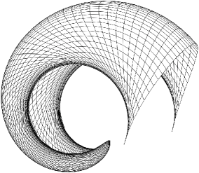
Figure 3: A transformed von Lilienthal surface.

Example 8.6.

Continuing the previous example, we describe the transformation of the corresponding orthogonal equiareal pattern. Under parameterization (27), the von Lilienthal solution $z=b^{2}-y^{2}$ generates the orthogonal equiareal pattern

$$\mathbf{I}_{\mathrm{Arch}}=\big{(}b^{2}-y^{2}\big{)}\,{\mathrm{d}}x^{2}+\frac{1}{b^{2}-y^{2}}\,{\mathrm{d}}y^{2}$$

known as the Archimedean projection.

The Gaussian image of the transformed surface is

$$\tilde{\mathbf{n}}_{1}=\frac{\sqrt{b^{2}-y^{2}}}{b}\frac{\big{(}x^{2}\big{(}b^{2}-y^{2}\big{)}-1\big{)}\cos(bx)-2xb\sin(bx)}{x^{2}\big{(}b^{2}-y^{2}\big{)}+1},$$

$$\tilde{\mathbf{n}}_{2}=\frac{\sqrt{b^{2}-y^{2}}}{b}\frac{(x^{2}\big{(}b^{2}-y^{2}\big{)}-1)\sin(bx)+2xb\cos(bx)}{x^{2}\big{(}b^{2}-y^{2}\big{)}+1},$$

$$\tilde{\mathbf{n}}_{3}=-\frac{y}{b}\frac{x^{2}\big{(}b^{2}-y^{2}\big{)}-1}{x^{2}\big{(}b^{2}-y^{2}\big{)}+1}.$$

To express the ${\mathcal{X}}$-transformed orthogonal equiareal pattern explicitly, one needs to invert the transformation $(x,y)\leftrightarrow(x^{\prime},y^{\prime})$, where $x^{\prime}$, $y^{\prime}$ are given by formula (26). The ${\mathcal{X}}$-transformed orthogonal equiareal pattern $\tilde{\mathbf{n}}^{\prime}(x^{\prime},y^{\prime})$ can be seen in the right part of Fig. 4.

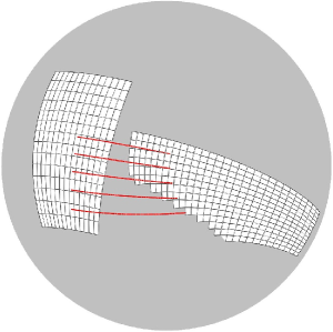
Figure 4: A part of Archimedean projection (left) and a part of its ${\mathcal{X}}$-transformed pattern (right) connected by great circles’ arcs (red).

Example 8.7.

A solution $z(x,y)$ is invariant under the scaling symmetry if

$$xz_{x}-yz_{y}+2z=0.$$

Consider the scaling invariant solutions

$$z=\frac{F}{x^{2}},\qquad\frac{x^{2}y^{2}}{F}+x^{2}y^{2}+F=a_{1}xy+a_{0}$$

obtained in [14, proof of Proposition 1]. Recall that the corresponding surface of constant astigmatism belongs to the Lipschitz class [18]. Since

$$F=-\frac{1}{2}x^{2}y^{2}+\frac{1}{2}a_{1}xy+\frac{1}{2}a_{0}+\frac{1}{2}\sqrt{x^{4}y^{4}-2a_{1}x^{3}y^{3}+\big{(}a_{1}^{2}-2a_{0}-4\big{)}x^{2}y^{2}+2a_{0}a_{1}xy+a_{0}^{2}}$$

computation of $\eta$ and $\xi$ will lead to elliptic integrals unless the discriminant

$$256a_{0}^{2}\big{(}a_{1}^{2}+4a_{0}+4a_{1}+4\big{)}\big{(}a_{1}^{2}+4a_{0}-4a_{1}+4\big{)}$$

of the polynomial under the square root is zero, i.e., unless $a_{0}=0$ or $a_{0}=-\big{(}\frac{1}{2}a_{1}\pm 1\big{)}^{2}$. To keep things simple, we restrict ourself to the easiest subcase $a_{1}=a_{0}=0$. Then

$$z=\frac{y\big{(}\sqrt{{x}^{2}{y}^{2}-4}-xy\big{)}}{2x}.$$

The potentials are

$$\chi=\sqrt{x^{2}y^{2}-4}+\arctan\frac{2}{\sqrt{x^{2}y^{2}-4}}+c_{1},\qquad\eta=\frac{1}{2}x\big{(}\sqrt{x^{2}y^{2}-4}-xy\big{)}+c_{2}.$$

Applying the transformation ${\mathcal{X}}$, we obtain

$$x^{\prime}=\frac{1}{2}xy^{2}+\frac{1}{2}y\sqrt{x^{2}y^{2}-4},\qquad y^{\prime}=-\frac{1}{2}x^{2}y+\frac{1}{2}x\sqrt{x^{2}y^{2}-4}+c_{2},$$

$$z^{\prime}=-\frac{1}{2}x^{4}y^{2}+\frac{1}{2}\left(x^{3}y-\frac{x}{y}\right)\sqrt{x^{2}y^{2}-4}+\frac{3}{2}x^{2}.$$

Is is easy to check that $z^{\prime}(x^{\prime},y^{\prime})$ satisfies $x^{\prime}z^{\prime}_{x^{\prime}}-y^{\prime}z^{\prime}_{y^{\prime}}+2z^{\prime}+2c_{2}z^{\prime}_{y^{\prime}}=0$, i.e., is invariant under a combination of the scaling symmetry and the $y$-translation. As such, $z^{\prime}(x^{\prime},y^{\prime})$ is just another Lipschitz solution.

Applying the transformation ${\mathcal{X}}_{\mathfrak{X}}$, see Section 5, we obtain the solution

$$x^{\prime}=\frac{(tx+1)\big{(}{-}xy+\sqrt{x^{2}y^{2}-4}\big{)}y+2tx}{(tx+1)^{2}\big{(}{-}xy+\sqrt{x^{2}y^{2}-4}\big{)}y+2t^{2}x},$$

$$y^{\prime}=-(tx+1)y+\left(-\frac{1}{2}x^{2}y+\frac{1}{2}x\sqrt{x^{2}y^{2}-4}+c_{2}\right)t^{2}$$

$$\hphantom{y^{\prime}=}{}+\left(\sqrt{x^{2}y^{2}-4}+\arctan\frac{2}{\sqrt{x^{2}y^{2}-4}}+c_{1}\right)t,$$

$$z^{\prime}=\frac{(tx+1)^{4}\big{(}\big{(}{-}xy+\sqrt{x^{2}y^{2}-4}\big{)}y+2t^{2}x^{2}\big{)}^{2}}{x^{3}y\big{(}{-}xy+\sqrt{x^{2}y^{2}-4}\big{)}}.$$

This solution is not invariant under any local symmetry.

Acknowledgements

We are indebted to I.S. Krasil’shchik for reading the manuscript and valuable comments. A.H. was supported by Silesian University in Opava under the student grant project SGS/1/2011, M.M. was supported by GAČR under project P201/11/0356.

References

[1]
Bäcklund A.V., Om ytor med konstant negativ krökning, Lunds Univ.
Årsskrift19 (1883), 1–48.
[3]
Baran H., Marvan M., Classification of integrable Weingarten surfaces
possessing an -valued zero curvature representation,
Nonlinearity23 (2010), 2577–2597, arXiv:1002.0992.
[4]
Bianchi L., Ricerche sulle superficie elicoidali e sulle superficie a curvatura
costante, Ann. Scuola Norm. Sup. Pisa Cl. Sci.2 (1879),
285–341.
[5]
Bianchi L., Lezioni di Geometria Differenziale, Vol. I, E. Spoerri, Pisa, 1902.
[6]
Bianchi L., Lezioni di Geometria Differenziale, Vol. II, E. Spoerri, Pisa,
1903.
[8]
Ferapontov E.V., Reciprocal transformations and their invariants,
Differ. Equ.25 (1989), 898–905.
[9]
Ferapontov E.V., Autotransformations with respect to the solution, and
hydrodynamic symmetries, Differ. Equ.27 (1991), 885–895.
[10]
Ferapontov E.V., Rogers C., Schief W.K., Reciprocal transformations of
two-component hyperbolic systems and their invariants, J. Math. Anal.
Appl.228 (1998), 365–376.
[11]
Ganchev G., Mihova V., On the invariant theory of Weingarten surfaces in
Euclidean space, J. Phys. A: Math. Theor.43 (2010),
405210, 27 pages, arXiv:0802.2191.
[12]
Goursat E., Le Probléme de Bäcklund, Gauthier-Villars, Paris, 1925.
[13]
Hlaváč A., Marvan M., Another integrable case in two-dimensional
plasticity, J. Phys. A: Math. Theor.46 (2013), 045203,
15 pages.
[14]
Hlaváč A., Marvan M., On Lipschitz solutions of the constant
astigmatism equation, J. Geom. Phys., to appear.
[15]
Hoenselaers C.A., Miccichè S., Transcendental solutions of the
sine-Gordon equation, in Bäcklund and Darboux Transformations. The
Geometry of Solitons (Halifax, NS, 1999), CRM Proc. Lecture
Notes, Vol. 29, Amer. Math. Soc., Providence, RI, 2001, 261–271.
[16]
Kingston J.G., Rogers C., Reciprocal Bäcklund transformations of
conservation laws, Phys. Lett. A92 (1982), 261–264.
[17]
von Lilienthal R., Bemerkung über diejenigen Flächen bei denen die
Differenz der Hauptkrümmungsradien constant ist, Acta Math.11 (1887), 391–394.
[18]
Lipschitz R., Zur Theorie der krummen Oberflächen, Acta Math.10 (1887), 131–136.
[23]
Prus R., Sym A., Rectilinear congruences and Bäcklund transformations:
roots of the soliton theory, in Nonlinearity & Geometry, Luigi Bianchi Days
(Warsaw, 1995), Editors D. Wójcik, J. Cieśliński, Polish Scientific
Publishers, Warsaw, 1998, 25–36.
[24]
Ribaucour A., Note sur les développées des surfaces, C. R. Math.
Acad. Sci. Paris74 (1872), 1399–1403.
[25]
Rogers C., Schief W.K., Bäcklund and Darboux transformations. Geometry and
modern applications in soliton theory, Cambridge Texts in Applied
Mathematics, Cambridge University Press, Cambridge, 2002.
[26]
Rogers C., Schief W.K., Szereszewski A., Loop soliton interaction in an
integrable nonlinear telegraphy model: reciprocal and Bäcklund
transformations, J. Phys. A: Math. Theor.43 (2010),
385210, 16 pages.
[27]
Rogers C., Shadwick W.F., Bäcklund transformations and their applications,
Mathematics in Science and Engineering, Vol. 161, Academic Press,
Inc., New York – London, 1982.
[28]
Rogers C., Wong P., On reciprocal Bäcklund transformations of inverse
scattering schemes, Phys. Scripta30 (1984), 10–14.
[29]
Sadowsky M.A., Equiareal pattern of stress trajectories in plane plastic
strain, J. Appl. Mech.8 (1941), A74–A76.