Revisiting algorithms for generating surrogate time series

Abstract

The method of surrogates is one of the key concepts of nonlinear data analysis. Here, we demonstrate that commonly used algorithms for generating surrogates often fail to generate truly linear time series. Rather, they create surrogate realizations with Fourier phase correlations leading to non-detections of nonlinearities. We argue that reliable surrogates can only be generated, if one tests separately for static and dynamic nonlinearities.

Introduction. The method of surrogates Theiler et al. (1992) is one of the the key concepts of nonlinear data analysis, which allows to test for weak nonlinearities in data sets in a model-independent way. The basic idea of this approach is to compute statistics sensitive to nonlinearities for the original data set and for an ensemble of so-called surrogate data sets, which mimic the linear properties of the original data. If the computed measure for the original data is significantly different from the values obtained for the set of surrogates, one can infer that the data contain nonlinearities.
Linearity means in this case that all the structure in the time series is contained in the autocorrelation function, or equivalently, in the Fourier power spectrum. Thus the time series $y_{t}$ can be modeled e.g. by an autoregressive (AR) model described by $y_{t}=a_{0}+\sum_{k=1}^{q}a_{k}y_{t-k}+\sigma e_{t}$ ($a$: coefficients, $e$: white noise) or a more general ARMA models also including moving averages (MA). Nonlinearity thus refers to all those structures in data sets that are not captured by the power spectrum.
Since its introduction the method of surrogates has found numerous applications in many fields of research ranging from geophysical and physiological time series analysis Schreiber and Schmitz (2000) to econophysics Wang et al. (2008), astrophysics Gliozzi et al. (2010), and cosmology Räth et al. (2009, 2011).
The most commonly used methods for generating surrogates include Fourier-transformed (FT), amplitude adjusted Fourier-transformed (AAFT) Theiler et al. (1992) and iterative amplitude adjusted Fourier-transformed (IAAFT) surrogates Schreiber and Schmitz (1996). With FT surrogates, which are generated by using the Fourier amplitudes of the original time series and a set of random phases, one tests whether the time series is compatible with a linear Gaussian process. In other words, any significant deviation of the original data from its surrogates indicates the presence of higher order temporal correlations, i.e. the presence of dynamic nonlinearities.
The null hypothesis can be generalized to cases where the data set is non-Gaussian. Here, the hypothesis is that the original data $\left\{y_{n}\right\}$ are from a nonlinear or linear stochastic process that has undergone a static nonlinear transformation. The AAFT algorithm was developed to generate this kind of surrogates. The original time series is rendered Gaussian by a rank-ordered remapping of the values onto a Gaussian distribution. For this Gaussian time series which follows the measured time evolution, a FT surrogate time series is generated. The final surrogate data are obtained by rank-ordered remapping of the FT surrogate onto the distribution of the original data.
It was shown that the final remapping step in the AAFT algorithm can lead to a whitening of the power spectrum Schreiber and Schmitz (1996). This shortcoming was overcome by the IAAFT algorithm, which consists of the following iteration scheme. (1) One starts with a random shuffle $\left\{y_{n}^{i}\right\}$ of the original data $\left\{y_{n}\right\}$, which is Fourier transformed yielding the Fourier amplitudes $\left|S^{i}(k)\right|$ and Fourier phases $\phi^{i}(k)$ . (2) The Fourier amplitudes $\left|S^{i}(k)\right|$ of the time series $\left\{y_{n}^{i}\right\}$ are then replaced by those for the original data $\left|Y(k)\right|=\left|\sum_{n=1}^{N}y_{n}e^{i2\pi kn/N}\right|$. The phases of the complex Fourier $\phi^{i}(k)$ components are kept. An inverse Fourier transformation leads to a time series with desired power spectrum $\left\{z_{n}^{i}\right\}$. (3) To make the surrogate time series have the same amplitude distribution $\left\{y_{n}\right\}$ in real space as the original data, $\left\{z_{n}^{i}\right\}$ is remapped in a rank ordered way onto $\left\{y_{n}^{i}\right\}$ leading to $\left\{y_{n}^{i+1}\right\}$. As in AAFT the final remapping step changes the power spectrum, so that steps (2) and (3) have to be repeated until convergence to the correct power spectrum is achieved. AAFT and IAAFT strive for a proper reproduction of the linear properties and the amplitude distribution of the time series. All three algorithms have in common that they intend to translate the absence of nonlinear temporal correlations into the constraint of uncorrelated and uniformly distributed phases in the Fourier representation of the data. While the randomness of the phases remains (by construction) exactly preserved for FT surrogates, it has never been studied, how the remapping step (in AAFT) and the iteration steps (in IAAFT) affect the randomness of the phases in the resulting surrogate time series.
In this Letter we investigate in detail how well this much more important constraint of the absence of nonlinear correlations in the surrogates is fulfilled for AAFT and IAAFT surrogates and study consequences for the outcome of tests on nonlinearity for observational data.

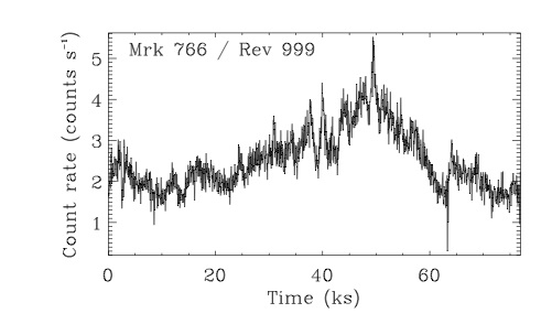
Data Set and Preprocessing. All following investigations are based on two – quite distinct – data sets. The first one is an X-ray observation of the narrow-line Seyfert 1 galaxy Mrk 766 taken with the XMM Newton satellite Markowitz et al. (2007). For light curves from active galactic nuclei (AGN) one investigates the linear and nonlinear temporal correlations to infer more information about the physical processes in the innermost regions of these compact accreting objects. The time series originates from observations of Mrk 766 in 2005. We selected the revolution 999 from May, 23rd, 2005 that took 95 ks. We used the data retrieved from the XMM public archive and only relied on data from the PN camera Strüder et al. (2001) due to its superior statistical quality. Source counts were accumulated from a rectangular box of 27 $\times$ 26 RAW pixels (1 RAW pixel $\sim$ 4.1 arcsec) around the position of the source. Background data were extracted from a similar, source free region on the chip. After rejection of times affected by high background a light curve was extracted in the 0.3$-$10 keV energy band, background subtracted and binned to 50 s time resolution.
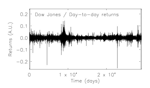
The second data set are the day-to-day returns of the Dow Jones (DJ) industrial index covering the period from 26th of May 1896 until 8th of June 2012. From the publicly available (www.djaverages.com) closing prices $p(t)$ of each trading day the day-to-day returns $r(t)$ are determined by considering the change of the logarithm of the stock price $r_{\Delta t}(t)=\ln(p(t))-\ln(p(t-\Delta t))$, where $\Delta t=1$ day. Both data sets (see Fig. 1) are particularly well suited to be used for testing concepts of nonlinear time series analysis, because they represent scalar, real time series from a sufficiently complex system, where the mere detection of nonlinearities already allows to discriminate between different classes of models. In the case of the the AGN-data comparably simple intrinsically linear models for light curve variations like e.g. global disk oscillations models Titarchuk and Osherovich (2000) can be safely ruled out. The detection of signatures of nonlinear determinism in financial data shows that the stock market is neither completely governed by stochastic processes nor can it be purely described by linear processes plus additive noise.

Figure 1: Light curve of the observation of Mrk 766 in 50 s time resolution (above) and the day-to-day returns of the Dow Jones Industrial index (below). The time series consists of $1540$ and $29070$ points respectively.

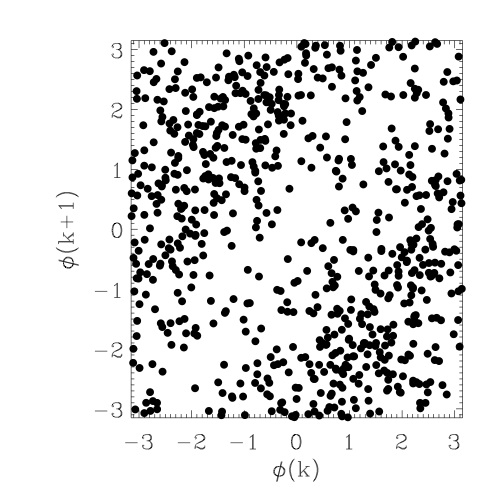
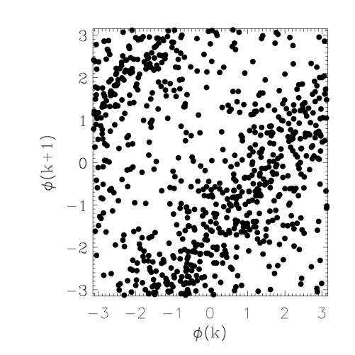
Analyses and Results. For both time series we generate 200 realizations of FT, AAFT and IAAFT surrogates each. Note that in the FT case the random phase hypothesis for the surrogates is doubtlessly fulfilled. To assess the presence or absence of nonlinear correlations in the surrogates we make use of the representation of Fourier phases in so-called phase maps Chiang et al. (2002). A phase map is defined as a two-dimensional set of points $G=\{\phi_{k},\phi_{k+\Delta}\}$ where $\phi_{k}$ is the phase of the $k^{th}$ mode of the Fourier transform and $\Delta$ a phase delay. 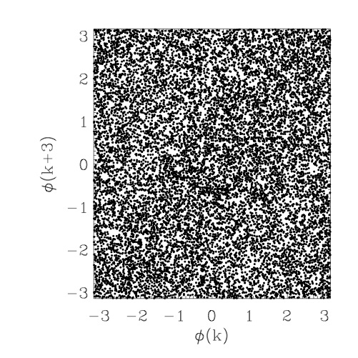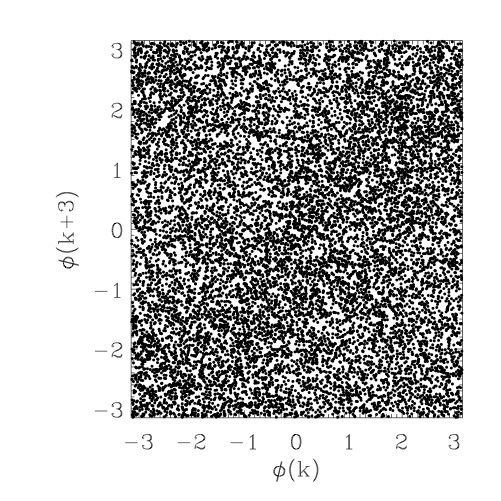If the phases were taken from a random, uniform and uncorrelated distribution, the phase maps $G$ would be a random two-dimensional distribution of points in the interval $\left[-\pi;\pi\right]$. Any significant deviation from this random distribution already points towards the presence of nonlinearities in the data. In Fig. 2 we show the phase maps for the AGN case for a delay $\Delta=1$ for one AAFT and one IAAFT realization. For the Dow Jones data we show the respective plots for $\Delta=3$. IFor both types of times series and for both classes of surrogates the phase maps are far from being random. 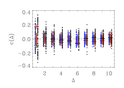To quantify the degree of correlation between the phases $\phi$ and $\phi+\Delta$ we calculate the correlation coefficient $c(\Delta)$ for delays up to $\Delta=10$. In Fig. 3 we show $c(\Delta)$ for the three classes of surrogates and both time series under study. The jitter around zero of the FT surrogates (red) represents – by construction – the statistical fluctuations of $c(\Delta)$ for a limited number of phases. For both examples, however, these fluctuations around zero are significantly larger for the AAFT surrogates (blue) and IAAFT surrogates (black) for a number of values of $\Delta$. This results in up to $138$ (IAAFT) and $110$ (AAFT) surrogate realizations leading to $c$-values lying outside the 3 $\sigma$ confidence region around zero. Since the only difference between FT and AAFT is the remapping step after the inverse Fourier transformation, we can immediately infer that this step is responsible for inducing the phase correlations. The deviations from zero for the correlation coefficient become in both cases more pronounced for the IAAFT surrogates. For the AGN light curve one can even observe that for $\Delta=1$ the region around zero for $c(\Delta)$ is thinned out meaning that it is rather a rule than an exception that $\left|c(\Delta)\right|$ becomes larger than the normal statistical fluctuations. The presence of phase correlations in the majority of surrogate realizations proves already in a strict mathematical sense that those realizations are in fact nonlinear.
To address the relationship between phase correlations and measures for nonlinearity we calculate the nonlinear prediction error (NPLE) as described in Sugihara and May (1990).

Figure 2: Phase maps for $\Delta=1$ for one AAFT (left) and one IAAFT (right) surrogate realization for the AGN time series (above). Below the phase maps for $\Delta=3$ for one AAFT (left) and one IAAFT (right) surrogate realization for the Dow Jones data are shown.

Figure 3: Cross-correlation between $\phi(k)$ and $\phi(k+\Delta)$ for $\Delta=1,\ldots,10$ for 100 realizations of FT (red), AAFT (blue) and IAAFT (black) surrogates for the Mrk 766 (above) and the Dow Jones (below) time series. The black (red) crosses denote the values for $c(\Delta)$ for the original time series (remapped original time series) for comparison.

The NLPE has been shown to be a robust measure with a good overall performance Schreiber and Schmitz (1997). The calculation of the NLPE relies on the representation of the time series in an artificial phase space, which is obtained using the method of delay coordinates Packard et al. (1980). This is accomplished by using time delayed versions of the observed time series as coordinates for the embedding space. The multivariate vectors in the $d$-dimensional space are expressed by $\vec{y}_{n}=(y_{n-(d-1)\tau},y_{n-(d-2)\tau},\ldots,y_{n})\;,$ where $\tau$ is the delay time and $y_{n}$ denotes the value of the (discretized) time series at time step $n$. The comparison of the predicted behavior of the time series based on the local neighbors with the real trajectory of the system leads to the definition of the NLPE $\psi$ as

$$\psi = \psi(d,\tau,T,N)$$

$$= \frac{1}{(M-T-(d-1)\tau)}\sqrt{\sum_{n=(d-1)\tau}^{M-1-T}[\vec{y}_{n+T}-F(\vec{y}_{n})]^{2}}$$

where $F$ is a locally constant predictor, $M$ is the length of the time series, and $T$ is the lead time. The predictor $F$ is calculated by averaging over future values of the $N\,(N=d+1)$ nearest neighbors in the delay coordinate representation.
We found that for $T>5$ $\psi$ remains rather constant, thus a value of $T=5$ was used for this study. The dimension of the embedding space $d$ and the delay time $\tau$ have to be set appropriately. Since the AGN time series of this study consist only of $1539$ data points , we use a low embedding dimension $d=3$, so that the vectors $\vec{y}_{n}$ are not too sparsely distributed in the embedding space. To allow for direct comparison we also used $d=3$ for the much longer time series of the Dow Jones.
The delay time $\tau$ is determined by using the criterion of zero crossing of the autocorrelation function or the first minimum of the autocorrelation function or mutual information Fraser and Swinney (1986), which lies around $\tau=10$ ks for Mrk 766 and $\tau=2$ days respectively. To also investigate the robustness of our results with respect to variations of $\tau$, we calculate the NPLE for a set of four different delay-times, $\tau=7.5,8.75,10.0$ and $11.25$ ks (AGN data) and $\tau=2,3,4$ and $5$ days (DJ data) and analyze the results as a function of $\tau$.
First, we investigated the relation between the phase correlations $c(\Delta)$ and the NLPE $\psi(\tau)$ for both time series. While no obvious trends between linear correlations in the phase maps and the nonlinear prediction error could be identified for the DJ data, we found remarkable anti-correlations for the AAFT ($-0.68$) and IAAFT ($-0.94$) between $c(\Delta=1)$ and $\psi(\tau=10ks)$ for the Mrk 766 data. The latter value means a nearly perfect correlation indicating that the NLPE calculated for IAAFT surrogates is mostly determined by Fourier phase correlations for $\Delta=1$. We note here that this kind of analysis has the potential to shed more light on the effects of phase correlations on the shape of the point distribution in embedding space to ultimately get more insight into the meaning of Fourier phases for nonlinear time series. For this study, however, it is already sufficient to show that there are significant phase correlations which affect the calculation of nonlinear statistics.
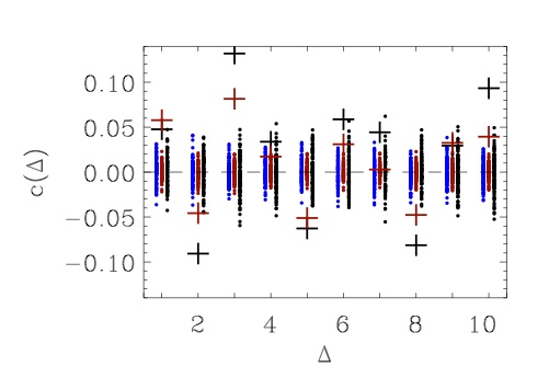
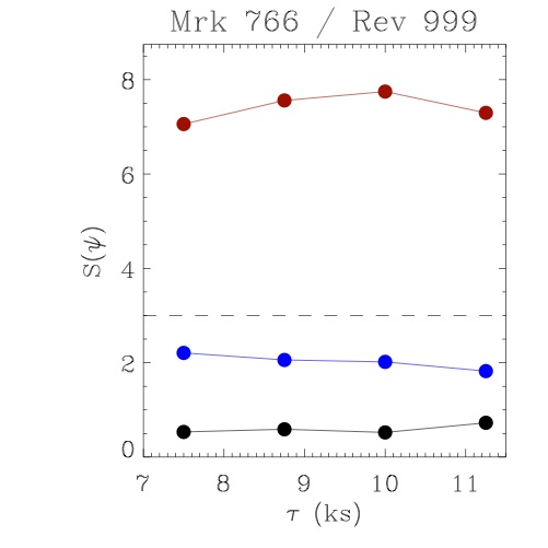
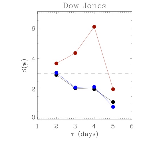
The results for a standard test on nonlinearities using the NLPE as test statistics are summarized in Fig. 4. We plot the significances $S(\psi)$,

$$S(\psi)=\left|\frac{\psi_{original}-\langle\psi\rangle_{surrogate}}{\sigma_{\psi_{surrogate}}}\right|\;,$$ (2)

as a function of $\tau$. The mean $\langle\psi\rangle_{surrogate}$ and the standard deviation $\sigma_{\psi_{surrogate}}$ are derived by summing over $N=200$ realizations of the respective set of surrogates. Obviously, the propagation of the phase correlations found for the AAFT and IAAFT surrogates to the calculation of the NLPE eventually leads to a non-detection of nonlinearities. For both time series the significances for the AAFT and IAAFT test are well below the 3 $\sigma$ detection criterion, whereas the test on dynamic nonlinearities using the remapped time series and FT surrogates yields a highly significant detection of nonlinearities with $S(\psi)$ reaching eight for Mrk 766 and six for the Dow Jones . These results remain stable for a range of delay times.

Figure 4: Significances $S(\psi)$ for nonlinear temporal correlations for the set of light curves as determined with NLPE and as a function of the delay time $\tau$ for Mrk 766 (left) and the Dow Jones (right). Red: results obtained using the remapped time series and FT surrogates. Black: results obtained with the original data and the ITAAFT algorithm. Blue: results for the original data and the AAFT algorithm. The dashed line indicates the 3 $\sigma$ detection limit.

Conclusions. Using the examples of an AGN light curve and the Dow Jones day-to-day returns we demonstrated that both the AAFT and IAAFT algorithm can generate surrogate data sets with phase correlations. Thus, these time series have to be considered as nonlinear. We further showed that those phase correlations propagate into the calculation of nonlinear statistics like the NLPE. Hence, nonlinearities in time series may remain undetected due to the presence of them in a number of surrogate realizations against which the original data are compared. The wrong outcome of the surrogate test leads then, in turn, to a wrong modeling of the complex underlying system. In our case the AAFT and IAAFT surrogate test would suggest that the X-ray variability of Mrk 766 is compatible with a global disk oscillations model, which is clearly ruled out by the FT surrogate test. Similarly, the detection of weak dynamic nonlinearities (only with FT-surrogates) proves once again that the returns are correlated with each other, which disproves one of the basic assumptions of the Black-Scholes model Black and Scholes (1973); Merton (1973), where they are assumed to be random and independent from each other. Since the correlations are nonlinear, simple ARMA processes cannot be used as market models. Finally, the detected nonlinearities for the remapped data represent signatures that go beyond the so-called stylised facts (see e.g. Bunde et al. (2002)) of the fluctuations of price indices, that mostly relate to the shape of the probability density derived from the original distribution of the return values, e. g. ’fat tails’ etc. Market models must thus not only be able to reproduce these features but must also account for the intrinsic dynamic nonlinearities detected by means of FT-surrogate test.
By analyzing a larger set of AGN light curves as well as other typical simulated nonlinear time series like e.g. the Lorenz system we convinced ourselves that the presence of phase correlations is a generic property of AAFT and IAAFT surrogates – rather independent of the underlying time series under study.
Having outlined the consequences of surrogate tests on model building using the examples of an AGN light curve and the Dow Jones day -to-day returns it becomes obvious that it may be necessary that previous results obtained with AAFT and IAAFT have to be critically reassessed. It may be that weak nonlinearities remained undetected when AAFT and IAAFT surrogates were used. As a consequence wrong physical models may have been found to be compatible with the data.
In general, surrogate generating algorithms aiming at testing both static and dynamic nonlinearities cannot reproduce both the power spectrum and the amplitude distribution while preserving the randomness of the Fourier phases so far. Thus, one has to test separately for static and dynamic nonlinearities. The latter can be achieved by using FT surrogates for remapped time series as a reliable and truly linear class of surrogates. Additional comparably easy tests on the Gaussianity of the amplitude distribution can exclude the presence of static nonlinearities induced by a nonlinear rescaling.
Acknowledgments. This work has made use of observations obtained with XMM-Newton, an ESA science mission with instruments and contributions directly funded by ESA member states and the US (NASA).

References

- Theiler et al. (1992) J. Theiler, S. Eubank, A. Longtin, B. Galdrikian, and J. D. Farmer, Physica D 58, 77 (1992).
- Schreiber and Schmitz (2000) T. Schreiber and A. Schmitz, Physica D Nonlinear Phenomena 142, 346 (2000).
- Wang et al. (2008) F. Wang, K. Yamasaki, S. Havlin, and H. E. Stanley, Phys. Rev. E 77, 016109 (2008).
- Gliozzi et al. (2010) M. Gliozzi, C. Räth, I. E. Papadakis, and P. Reig, Astron. & Astrophys. 512, A21+ (2010).
- Räth et al. (2009) C. Räth, G. E. Morfill, G. Rossmanith, A. J. Banday, and K. M. Górski, Physical Review Letters 102, 131301 (2009).
- Räth et al. (2011) C. Räth, A. J. Banday, G. Rossmanith, H. Modest, R. Sütterlin, K. M. Górski, J. Delabrouille, and G. E. Morfill, Mon. Not. R. Astron. Soc. 415, 2205 (2011).
- Schreiber and Schmitz (1996) T. Schreiber and A. Schmitz, Phys. Rev. Lett. 77, 635 (1996).
- Markowitz et al. (2007) A. Markowitz, I. Papadakis, P. Arévalo, T. J. Turner, L. Miller, and J. N. Reeves, Astrophys. J. 656, 116 (2007).
- Strüder et al. (2001) L. Strüder, U. Briel, K. Dennerl, R. Hartmann, E. Kendziorra, N. Meidinger, E. Pfeffermann, C. Reppin, B. Aschenbach, W. Bornemann, et al., Astron. & Astrophys. 365, L18 (2001).
- Titarchuk and Osherovich (2000) L. Titarchuk and V. Osherovich, ApJL 542, L111 (2000).
- Chiang et al. (2002) L.-Y. Chiang, P. Coles, and P. Naselsky, Mon. Not. R. Astron. Soc. 337, 488 (2002).
- Sugihara and May (1990) G. Sugihara and R. M. May, Nature (London) 344, 734 (1990).
- Schreiber and Schmitz (1997) T. Schreiber and A. Schmitz, Phys. Rev. E 55, 5443 (1997).
- Packard et al. (1980) N. H. Packard, J. P. Crutchfield, J. D. Farmer, and R. S. Shaw, Physical Review Letters 45, 712 (1980).
- Fraser and Swinney (1986) A. M. Fraser and H. L. Swinney, Phys. Rev. A 33, 1134 (1986).
- Black and Scholes (1973) F. Black and M. Scholes, Journal of Political Economy 83, 637 (1973).
- Merton (1973) R. Merton, The Bell Journal of Economics and Management Science 4, 141 (1973).
- Bunde et al. (2002) A. Bunde, H. J. Schellnhuber, and J. Kropp, eds., The Science of Disasters: Climate Disruptions, Heart Attacks, and Market Crashes (Springer, Berlin, 2002).