Max-plus objects to study the complexity of graphs

Abstract

Given an undirected graph $G$, we define a new object $H_{G}$, called the mp-chart of $G$, in the max-plus algebra. We use it, together with the max-plus permanent, to describe the complexity of graphs. We show how to compute the mean and the variance of $H_{G}$ in terms of the adjacency matrix of $G$ and we give a central limit theorem for $H_{G}$. Finally, we show that the mp-chart is easily tractable also for the complement graph.

1 Introduction

The work presented in this paper has been inspired by the need of simple and actual techniques to measure the complexity of a graph, especially in the case of sparse graphs. This problem arises in several fields of applications, from Computer Science to Economics, from Biology to Social Sciences. As general references for the graph theory, we mention in particular the books [7], [8], [5] and [10], where the reader can find the main mathematical achievements in the theory. For a general survey on recent applications of graph theory see, for instance, [1]. The reader interested in some more technical papers can refer to [16] for applications to Economics, to [9] for applications to Econophysics, to [17] for applications to Biology, and to [15] for applications to Molecular Biology. In such papers, sparse graphs play a prominent role.

Although an undirected graph $G=(V,E)$ is a rather simple structure, consisting of a set $V$ of $N$ vertices and a set of edges $E\subset V\times V$, in graph theory there are several different approaches, depending on the specific application we are looking for. In particular, a graph can be fixed or random, depending on whether the elements in $E$ are random or not. Moreover, many efforts have been done to analyze dynamical graphs, where the vertex set $V$ and/or the edge set $E$ vary with time, see e.g. [11].

Here, we restrict our analysis to fixed graphs. In this framework, there are interesting developments in the area of Combinatorics, about the study of the properties of $0-1$ matrices. These matrices naturally arise in the framework of graphs, as the adjacency matrix $A_{G}$ of the fixed graph $G$. Some recent developments in this direction, with applications to graph theory, are described in [2], [3], and [4].

In the present paper, we investigate some questions about undirected graph, in order to study and describe their structure, with special attention to sparse graphs. Our work is related to the matching problem. As a preliminary remark, we argue that, for sparse graphs, the classical descriptors of the complexity, such as the degree distribution and the permanent of the adjacency matrix do not give actual information. Thus, we use the max-plus arithmetic and the corresponding expression of the permanent, and we show that this object is more suitable for describing of the complexity for sparse graph. The use of the max-plus arithmetic naturally leads to the definition of a more complete index of the structure of a graph, and we define a vector called the mp-chart of the graph. This vector is nothing else but a probability distribution, and we show that it converges to a Normal distribution through a combinatorial Central Limit Theorem. Several examples on small- and medium-sized graphs are given to show that our definitions are easy to apply and provide practical information about the complexity of the structure of the graph under study. All the computations have been carried out with Maple, see [18], and R, see [19]. All the simulations come from simple R routines, without any additional package.

This paper is only concerned with undirected fixed graphs. Nevertheless, the same strategy can be applied to other situations, such as bipartite graphs, undirected unfixed graphs, random graphs, and so on.

The paper is organized as follows. In Section 2 we define the max-plus permanent of an adjacency matrix (i.e., the permanent under the max-plus arithmetic), we state its main properties, we study its connections with the classical permanent, and we discuss some simple examples. In Section 3 we define a new object associated to a graph, and we call it the mp-chart of the graph. We compute its mean and variance, and we show that, under suitable conditions, it converges to a Normal distribution as the size of the graph goes to infinity. Some simple simulations show that the convergence is quite good also for small values of the size. In Section 4, we show how the mp-chart of a graph is related to the mp-chart of the complement graph. Finally, Section 5 is devoted to suggest some future directions of this research.

2 The max-plus permanent

Let $G=(V,E)$ be an undirected graph with $N$ vertices. Let $A_{G}$ be the $N\times N$ adjacency matrix of $G$, defined by $(A_{G})_{i,j}=1$ if $(i,j)\in E$ and $0$ otherwise. In the classic definition of undirected graph, the matrix $A_{G}$ is symmetric and with zero diagonal entries, as we do not consider loops.

As mentioned in the Introduction, the study of the complexity of a given graph is one of the most relevant problems about graphs in Applied Probability. This analysis can be performed through the distribution of the degrees (i.e., the number of edges involving each vertex) and through the permanent (or the determinant) of the adjacency matrix $A_{G}$.

The determinant of $A_{G}$ is

$$\mathrm{det}(A_{G})=\sum_{\pi}(-1)^{|\pi|}\prod_{i=1}^{N}(A_{G})_{i,\pi(i)}\,,$$

where the sum is taken over all the permutations $\pi$ of $\{1,\ldots,N\}$ and $|\pi|$ denotes the parity of $\pi$. The permanent of $A_{G}$ is

$$\mathrm{perm}(A_{G})=\sum_{\pi}\prod_{i=1}^{N}(A_{G})_{i,\pi(i)}\,.$$

The use of permanent to describe the complexity of a graph is justified by the following well-known property.

Proposition 1.

The permanent of $A_{G}$ is the number of bijections $\phi:V\rightarrow V$ compatible with $E$, i.e. such that $(v,\phi(v))\in E$ for all $v\in V$.

In fact, $\mathrm{perm}(A_{G})$ is the number of permutations $\pi$ with $A_{1,\pi(1)}=\ldots=A_{N,\pi(N)}=1$ and the permutation $\pi$ is just the bijection $\phi$ in the proposition.

However, the analysis based on the degree distribution and the permanent is not adequate for sparse graphs. In fact, it is enough to have an isolated vertex to produce a null permanent. Nevertheless, it is interesting to study the structure of a sparse graph.

To overcome this difficulty, we make use of the tropicalization of the permanent. In the classical settings, Tropical Arithmetic is defined through the operations:

$$x\oplus y=\min\{x,y\}\qquad x\otimes y=x+y$$

But, with Tropical Arithmetic, the determinant (or permanent) of an adjacency matrix is always $0$, because of the nullity of the main diagonal of $A_{G}$.

Thus, we use the max-plus algebra, with operations:

$$x\oplus y=\max\{x,y\}\qquad x\otimes y=x+y$$

Consequently, the explicit expression of the max-plus permanent is

$$\mathrm{perm_{mp}}(A_{G}):=\bigoplus_{\pi}\left(\bigotimes_{i=1}^{N}(A_{G})_{i,\pi(i)}\right)=\max_{\pi}\sum_{i=1}^{N}(A_{G})_{i,\pi(i)}$$ (1)

The max-plus permanent is the maximum over $N!$ terms. Each of the $N!$ terms is the sum of $N$ terms in $\{0,1\}$. Thus, the max-plus permanent $\mathrm{perm_{mp}}(A_{G})$ is zero if and only if the matrix $A_{G}$ is the null matrix. On the opposite side, the maximum allowed value of the max-plus permanent is $N$.

The use of the max-plus permanent to analyze sparse graphs has a first reason in the following property.

Lemma 2.

The following relation holds:

$$\mathrm{perm_{mp}}(A_{G})=N\Longleftrightarrow\mathrm{perm}(A_{G})>0\,.$$ (2)

Proof.

$\mathrm{perm_{mp}}(A_{G})=N$ if and only if there exists a permutation $\pi$ such that $\sum_{i=1}^{N}(A_{G})_{i,\pi(i)}=N$. This happens if and only if there exists $\pi$ such that $(A_{G})_{i,\pi(i)}=1$ for $i=1,\dots,N$, i.e. if and only if $\mathrm{perm}(A_{G})>0$. ∎

Remark 3.

Notice that, from Lemma 2 and from the previous discussion, it follows that the max-plus permanent is able to discriminate among graphs with standard permanent equal to zero.

Moreover, we explicitly write the following consistency property, whose simple proof is straightforward.

Lemma 4.

Let $G$ and $H$ be two graphs on two disjoint sets of vertices. Then,

$$\mathrm{perm_{mp}}(A_{G\cup H})=\mathrm{perm_{mp}}(A_{G})+\mathrm{perm_{mp}}(A_{H})\,.$$ (3)

The max-plus permanent has interesting connections with the subgraphs. Let $G^{\prime}=(V^{\prime},E^{\prime})$ a graph. If $V^{\prime}\subset V$ and $E^{\prime}\subset E$, then $G^{\prime}$ is a subgraph of $G=(V,E)$. A subgraph $G^{\prime}=(V^{\prime},E^{\prime})$ is the subgraph induced by $V^{\prime}$ if $E^{\prime}$ contains all the edges in $E$ involving the vertices in $V^{\prime}$. In order to analyze the max-plus permanent, in view of Equation (1), we introduce here the notion of $t$-term, which is strictly related to the subgraphs of $G$. Such connections will be studied later in this section.

Definition 5.

Given a graph $G$ with adjacency matrix $A_{G}$, a $t$-term is a sequence of indices $(i_{1},j_{1})\cdots(i_{t},j_{t})$ with

• $1\leq i_{1}<\ldots<i_{t}\leq N$;

• the $j_{k}$’s, with $1\leq j_{k}\leq N$ are all distinct;

• $(A_{G})_{i_{k},j_{k}}=1$ for all $k$.

For a $t$-term $P$, we denote $I(P)=\{i_{1},\dots,i_{t}\}$ and $J(P)=\{j_{1},\dots,j_{t}\}$.

Roughly speaking, a $t$-term corresponds to a sequence of positions of $t$ ones in the permutations. A straightforward consequence is the following statement.

Proposition 6.

The max-plus permanent of $G$ is $q$ if and only if there exists a $q$-term and there are no $t$-term with $t>q$.

Proposition 7.

Let $t$ the maximum integer such that there exists a $t$-term, then there exists a $t$-term $P$ such that $I(P)=J(P)$.

Proof.

We prove the statement by induction on $t$. If $t=2$ there is nothing to prove since if the $2$-term is given by $(i_{1},j_{1})(i_{2},j_{2})$ it is enough to consider the $2$-term $(i_{1},j_{1})(j_{1},i_{1})$.

Consider now a $t$-term $Q$ and suppose there exists a $k$ such that $i_{k}$ is in $I(Q)\setminus J(Q)$. First of all we notice that $j_{k}$ must be in $I(Q)$. If not, we can add the element $(j_{k},i_{k})$ to $Q$ obtaining a $(t+1)$-term which is a contradiction, since $Q$ is maximal. Hence, since $j_{k}\in I(Q)$ then there exists a $s$ such that $j_{k}=i_{s}\in I(Q)$. Then, we substitute $(i_{s},j_{s})$ with $(j_{k},i_{k})$ in our $t$-term and we obtain a new $t$-term of the form $(i_{k},j_{k})(j_{k},i_{k})Q^{\prime}$ where $Q^{\prime}$ is a $(t-2)$-term. This term $Q^{\prime}$ arises from the sub-matrix $A^{\prime}$ of $A(G)$ where we remove rows and columns $i_{k}$ and $j_{k}$. Hence $Q^{\prime}$ is a maximal $(t-2)$-term for $A^{\prime}$. By induction, the proof follows. ∎

Remark 8.

If $P$ is a $3$-term, then we must have $I(P)=J(P)$. In fact, if $P$ is $(i_{1},j_{1})(i_{2},j_{2})(i_{3},j_{3})$ with $I(P)\not=J(P)$ then, by the previous proposition, we obtain a new $3-$term $(i_{k},j_{k})(j_{k},i_{k})(i_{3},j_{3})$. Then it would be possible to extend it to $(i_{k},j_{k}),(j_{k},i_{k})(i_{3},j_{3})(j_{3},i_{3})$ against the maximality of $P$.

Remark 9.

In view of Proposition 7, the max-plus permanent is the cardinality of the largest subset of $V$ with a bijection compatible with $E$. This is another way to see that the max-plus permanent is able to detect the complexity of the graphs with null classical permanent.

Denote by $\ell_{G}$ the number of edges of a graph $G$. Among the subgraphs of Proposition 7, we are mainly interested in the ones with a minimal number of edges. These subgraphs are maximal in term of $\mathrm{perm_{mp}}{(A_{G^{\prime}})}$, but minimal in term of $\ell_{G^{\prime}}$. We made this more precise by the following definition.

Definition 10.

An mp-maximal subgraph $G^{\prime}$ of a graph $G$, is a subgraph of $G$ with $q=\mathrm{perm_{mp}}(A_{G})$ vertices,

$$\mathrm{perm_{mp}}(A_{G^{\prime}})=\mathrm{perm_{mp}}(A_{G})$$ (4)

and for all other subgraph $G^{\prime\prime}$ of $G$ satisfying (4) one has $\ell_{G^{\prime}}\leq\ell_{G^{\prime\prime}}$.

The rest of this section is devoted to the discussion of some examples and some useful remarks. In order to understand the definitions introduced above, we start with some small graphs.

Example 11.

Let us analyze the three graphs on $4$ vertices drawn in Figure 1. Their adjacency matrices are respectively

$$A_{G_{1}}=\begin{pmatrix}0&1&0&1\\ 1&0&1&0\\ 0&1&0&1\\ 1&0&1&0\end{pmatrix}\qquad A_{G_{2}}=\begin{pmatrix}0&1&0&0\\ 1&0&0&0\\ 0&0&0&1\\ 0&0&1&0\end{pmatrix}\qquad A_{G_{3}}=\begin{pmatrix}0&1&1&0\\ 1&0&1&0\\ 1&1&0&0\\ 0&0&0&0\end{pmatrix}$$

In the first graph, all vertices are connected and $\mathrm{perm_{mp}}(A_{G_{1}})=4$. However, this is not the minimal way to obtain a max-plus permanent equal to $4$. In fact, it is easy to check that $\mathrm{perm_{mp}}(A_{G_{2}})=4$. Thus the graph $G_{2}$ represents a mp-maximal subgraph for the graph $G_{1}$, but it is not the only one. If we look now at the graph $G_{3}$, we notice that there is a cycle of length $3$ and an isolated vertex. In such case, we have $\mathrm{perm_{mp}}(A_{G_{3}})=3$, and there is only one mp-maximal subgraph.

$G_{1}$		$G_{2}$		$G_{3}$

Fig. 1: The graphs $G_{1}$, $G_{2}$ and $G_{3}$ for Example 11.

Example 12.

To illustrate the behavior of the max-plus permanent and of the mp-maximal subgraphs, we analyze two opposite examples. with the same length. The two graphs are drawn in Figure 2. The graph $G_{1}$ on the left is the union of a tree and two isolated vertices, with $\mathrm{perm_{mp}}(A_{G_{1}})=2$ and $4$ maximal subgraphs with two vertices and one edge each. On the opposite side, the graph $G_{2}$ has a perfect matching, $\mathrm{perm_{mp}}(A_{G_{2}})=6$ and there is only $1$ maximal subgraph, i.e., the graph $G_{2}$ itself.

$G_{1}$		$G_{2}$

Fig. 2: The two graphs $G_{1}$ and $G_{2}$ for Example 12.

Proposition 13.

Two mp-maximal subgraphs are not disjoint.

Proof.

Consider a graph $G$ such that $\mathrm{perm_{mp}}(A_{G})=t$ and let $G^{\prime}=(V^{\prime},E^{\prime})$ and $G^{\prime\prime}=(V^{\prime\prime},E^{\prime\prime})$ be two mp-maximal subgraphs of $G$ with $t$ vertices each. Suppose that $V^{\prime}$ and $V^{\prime\prime}$ are disjoint. Then, by Formula (3), the adjacency matrix of $G^{\prime}\cup G^{\prime\prime}$ has max-plus permanent $2t$. Then $\mathrm{perm_{mp}}(A_{G})\geq 2t$ which is a contradiction. ∎

Remark 14.

In the max-plus arithmetic, the definition of determinant is not unique, see [13]. Therefore, one has to define the positive and negative determinant. In particular, the positive max-plus determinant is the maximum of the sums $\sum_{i}A_{i,\pi(i)}$ over all even permutations $\pi$. The negative determinant is defined by taking the odd permutations instead of the even ones. This issue is another reason to use the permanent instead of the determinant in the max-plus environment.

3 The mp-chart of a graph

The information about a graph is not contained only in the max-plus permanent, but in the whole distribution of the $N!$ terms $\sum_{i=1}^{N}(A_{G})_{i,\pi(i)}$. Thus, in this section we define the mp-chart of a graph as the distribution of the $N!$ terms above, and we prove that this distribution converges to a Gaussian distribution through the Hoeffding’s combinatorial central limit theorem, see [14]. We also show that the mean and the variance of that distribution can be computed easily from the adjacency matrix.

Definition 15.

Let $G$ be a graph and $A_{G}$ its adjacency matrix. Let $h_{G}(k)$ be the number of permutations $\pi$ such that $\sum_{i=1}^{N}(A_{G})_{i,\pi(i)}=k$. We call the $(N+1)$-dimensional integer vector $H_{G}=(h_{G}(0),\dots,h_{G}(N))$ the mp-chart of the graph $G$.

This object captures many features of the graph and has some relevant theoretical properties. To understand the meaning of $H_{G}$, notice that $h_{G}(k)$ is just the number of permutations $\pi$ such that the sequence $(A_{G})_{1,\pi(1)},\ldots,(A_{G})_{N,\pi(N)}$ contains a $k$-term but not a $(k+1)$-term. This gives precisely the meaning and the usefulness of the notion of random permutation in that context.

Example 16.

We use here a very simple scheme inspired by Econophysics, see [21] and [12]. Consider a population with $N$ agents, each possessing one good. The goods can be sent and received only along the edges of a graph $G$ and each agent can possess only one good. Given a random permutation $\pi$ of $\{1,\ldots,N\}$, the $i$-th agent can send its good to $\pi(i)$ if it receive a good from $\pi^{-1}(i)$. The quantity $\sum_{i=1}^{N}(A_{G})_{i,\pi(i)}$ is exactly the number of agents involved in this process. Of course, similar examples can be adapted to many other sciences.

We start the analysis of the mp-chart with the study of the mean $\mathbb{E}(H_{G})$ and the variance $\mathbb{V}(H_{G})$. Although these computations could be carried out applying Theorem 2 in [14], it is useful to state explicitly the proof for adjacency matrices.

Given an adjacency matrix $A=(A_{G})$, note that, for a random permutation $\pi$, the object

$$S_{N}(\pi)=A_{1,\pi(1)}+\ldots+A_{N,\pi(N)}$$ (5)

is the sum of $N$ binary random variables, and $A_{i,\pi(i)}$ is the addendum chosen in the $i$-th row of the adjacency matrix.

In order to analyze the mean of $H_{G}$, defined by

$$\mathbb{E}(H_{G})=\frac{\sum_{t=0}^{N}kh_{G}(k)}{N!}\,,$$ (6)

it is convenient to adopt an inductive approach.

Theorem 17.

The mean of the mp-chart $H_{G}$ is

$$\mathbb{E}(H_{G})=\frac{2\ell_{G}}{N}\,,$$ (7)

where $\ell_{G}$ is the number of edges in the graph $G$.

Proof.

Clearly, if $A_{G}$ is the null matrix, then $\mathbb{E}(H_{G})=0$. Suppose that the formula (7) holds true for $\ell_{G}-1$. By direct inspection, adding one edge has the following consequences. Among the $N!$ terms $S_{N}(\pi)$:

• $(N-2)!$ of them increase by $2$;

• $2(N-2)(N-2)!$ of them increase by $1$;

• the remaining $((N-2)^{2}+N-1)(N-2)!$ do not change.

Thus,

$$\mathbb{E}(H_{G})=\frac{2(\ell_{G}-1)}{N}+\frac{2(N-2)!+2(N-2)(N-2)!}{N!}=\frac{2(\ell_{G}-1)}{N}+\frac{2}{N}=\frac{2\ell_{G}}{N}\,.$$

∎

Example 18.

Given a complete graph $G$, its adjacency matrix has $0$ on the diagonal and $1$ elsewhere. The graph has ${N(N-1)}/{2}$ edges. Hence $\mathbb{E}(H_{G})=N-1$ which is the maximum allowed.

Notice that the mean $\mathbb{E}(H_{G})$ depends only in the number of edges of $G$, whatever they are collocated, that is, $\mathbb{E}(H_{G})$ does not take into account the topology of the graph. On the other hand, the variance $\mathbb{V}(H_{G})$ depends on the position of the edges.

Theorem 19.

The variance of the mp-chart $H_{G}$ is

$$\mathbb{V}(H_{G})=\sum_{i=1}^{N}\frac{d_{i}(N-d_{i})}{N^{2}}+\sum_{\begin{subarray}{c}i,j=1\\ i\neq j\end{subarray}}^{N}\frac{d_{i}d_{j}-NT_{i,j}}{N^{2}(N-1)}\,,$$ (8)

where $d_{1},\ldots,d_{N}$ are the degrees of the vertices and $T_{i,j}=<r_{i},r_{j}>$ is the scalar product of the $i$-th and the $j$-th row of $A_{G}$.

Proof.

By direct computation, the formula (8) holds for $N\leq 2$.

To prove the validity of Eq. (8) for $N\geq 3$, it is enough to compute the covariances

$$\mathrm{Cov}(A_{i,\pi(i)},A_{j,\pi(j)}) = \mathbb{E}(A_{i,\pi(i)}A_{j,\pi(j)})-d_{i}d_{j}/N^{2}=$$

$$= \mathbb{P}(A_{i,\pi(i)}=1,A_{j,\pi(j)}=1)-d_{i}d_{j}/N^{2}\,.$$

Without loss of generality we can fix $i=1$ and $j=2$ and we write for brevity $A_{1}$ for $A_{1,\pi(1)}$ and $A_{2}$ for $A_{2,\pi(2)}$. Moreover, we suppose that $d_{1}$ and $d_{2}$ are both non zero. (If $d_{1}=0$ or $d_{2}=0$, then trivially $\mathrm{Cov}(A_{1},A_{2})=0)$.

We divide the computation in two cases, and to help the reader we have sketched the two cases in Figure 3.

$\left(\begin{array}[]{cc|ccccc}0&0&&\cdots&&\cdots&\\ 0&0&&\cdots&&\cdots&\\ \hline\cr&&&&&&\\ \vdots&\vdots&&&&&\\ &&&&&\\ \vdots&\vdots&&&&\\ &\end{array}\right)$	$\left(\begin{array}[]{cc|ccccc}0&1&&\cdots&&\cdots&\\ 1&0&&\cdots&&\cdots&\\ \hline\cr&&&&&&\\ \vdots&\vdots&&&&&\\ &&&&&\\ \vdots&\vdots&&&&\\ &\end{array}\right)$
Case $(a)$	Case $(b)$

Fig. 3: The two cases arising in the proof of Theorem 19.

• Case $(a)$: $(1,2)$ is not an edge of the graph.Then:

  • there are $2(N-1)!$ permutations such that $\pi(1)=1$ or $\pi(1)=2$. For all these cases, $(A_{1}=1,A_{2}=1)$ is impossible;

  • there are $2(N-2)(N-2)!$ permutations such that $\pi(1)>2$, but $\pi(2)=1$ or $\pi(2)=2$. Also in all these cases, $(A_{1}=1,A_{2}=1)$ is impossible;

  • there are $(N-2)(N-3)(N-2)!$ permutations such that $\pi(1)>2$ and $\pi(2)>2$, and among these permutations

    $$(T_{1,2}d_{2}+(d_{1}-T_{1,2})d_{2})(N-2)!=(d_{1}d_{2}-T_{1,2})(N-2)!$$

    are such that $A_{1}A_{2}=1$.

  Therefore,

  $$\mathrm{Cov}(A_{1},A_{2})=\frac{d_{1}d_{2}-NT_{1,2}}{N^{2}(N-1)}$$

• Case $(b)$: $(1,2)$ is an edge of the graph. Then:

  • there are $(N-1)!$ permutations such that $\pi(1)=1$. In all such cases, $(A_{1}=1,A_{2}=1)$ is impossible;

  • there are $(N-2)!$ permutations such that $\pi(1)=2$ and $\pi(2)=1$. For such permutations, $A_{1}=1$ and $A_{2}=1$;

  • there are $(N-2)(N-2)!$ permutations such that $\pi(1)=2$ and $\pi(2)>2$. Among these permutations, $(d_{2}-1)(N-2)!$ are such that $A_{1}A_{2}=1$.

  • there are $(N-2)(N-2)!$ permutations such that $\pi(1)>2$ and $\pi(2)=1$. Among these permutations, $(d_{1}-1)(N-2)!$ are such that $A_{1}A_{2}=1$.

  • there are $(N-2)(N-2)!$ permutations such that $\pi(1)>2$ and $\pi(2)=2$. In all such cases, $A_{1}A_{2}=0$.

  • there are $(N-2)(N-3)(N-2)!$ permutations such that $\pi(1)>2$ and $\pi(2)>2$, and among these

    $$\begin{split}(T_{1,2}(d_{2}-2)+(d_{1}-1-T_{1,2})(d_{2}-1))(N-2)!=\\ =(d_{1}d_{2}-d_{1}-d_{2}-T_{1,2}+1)(N-2)!\end{split}$$

    are such that $A_{1}A_{2}=1$.

  Therefore, adding up all the contributions, we obtain again

  $$\mathrm{Cov}(A_{1},A_{2})=\frac{d_{1}d_{2}-NT_{1,2}}{N^{2}(N-1)}$$

The formula in Eq. (8) is now straightforward. ∎

Example 20.

Consider the matrices

$$A_{G_{1}}=\begin{pmatrix}0&1&0&0&0\\ 1&0&1&0&0\\ 0&1&0&0&0\\ 0&0&0&0&0\\ 0&0&0&0&0\end{pmatrix}\qquad A_{G_{2}}=\begin{pmatrix}0&1&0&0&0\\ 1&0&0&0&0\\ 0&0&0&1&0\\ 0&0&1&0&0\\ 0&0&0&0&0\end{pmatrix}$$

The graph $G_{1}$ has two consecutive edges, while the graph $G_{2}$ has two disjoint edges. An easy computation gives

$$H_{G_{1}}=(48,48,24,0,0,0)$$

and

$$H_{G_{2}}=(53,44,18,4,1,0)$$

with equal means $\mathbb{E}(H_{G_{1}})=\mathbb{E}(H_{G_{2}})={4}/{5}$. On the contrary, the variances are $\mathbb{V}(H_{G_{1}})={14}/{25}$ and $\mathbb{V}(H_{G_{2}})={19}/{25}$, respectively.

Example 21.

As a second example, consider the two graphs on the set vertices $V=\{1,\ldots,7\}$ shown in Figure 4.

$G_{1}$		$G_{2}$

Fig. 4: Two graphs with different mp-charts, but with equal means and variances.

Notice that $G_{1}$ and $G_{2}$ differ by only one edge. The two mp-charts $H_{G_{1}}$ and $H_{G_{2}}$ have the same mean and variance, namely

$${\mathbb{E}}(H_{G_{1}})={\mathbb{E}}(H_{G_{2}})=\frac{12}{7}\qquad\qquad{\mathbb{V}}(H_{G_{1}})={\mathbb{V}}(H_{G_{2}})=\frac{170}{147}$$

but the mp-charts are different:

$$H_{G_{1}} = (678,1512,1716,840,294,0,0,0)$$

$$H_{G_{2}} = (674,1480,1792,840,218,32,4,0)\,.$$

The results above lead to a central limit theorem.

Theorem 22.

Let $G_{N}$ be a graph with $N$ vertices and let $A_{G_{N}}$ be its adjacency matrix. Let $\pi$ be a random permutation of $\{1,\ldots,N\}$ chosen with uniform probability and define

$$S_{N}(\pi)=\sum_{i=1}^{N}(A_{G_{N}})_{i,\pi(i)}\,.$$ (9)

If $\mathbb{V}(S_{N})$ goes to infinity as $N\rightarrow\infty$, then the distribution of $S_{N}$ is asymptotically normal.

Proof.

We make use of Theorem 3 in [14]. Define the auxiliary matrix $R$ with elements

$$R_{i,j}=(A_{G_{N}})_{i,j}-\frac{d_{i}}{N}-\frac{d_{j}}{N}+\frac{1}{N^{2}}\sum_{h,k}(A_{G_{N}})_{h,k}$$ (10)

Then, a sufficient condition for the asymptotic normality is that

$$\lim_{N\rightarrow\infty}\frac{\max_{1\leq i,j\leq N}R^{2}_{i,j}}{\frac{1}{N}\sum_{i,j=1}^{N}R^{2}_{i,j}}=0\,.$$ (11)

Now observe that the numerator is bounded, as $-2\leq R_{i,j}\leq 2$ for all $i$ and $j$. Moreover, Theorem 2 in the same paper [14] states that

$$\mathbb{V}(S_{N})=\frac{1}{N-1}\sum_{i,j=1}^{N}R_{i,j}^{2}\,.$$ (12)

Combining these facts, the result follows. ∎

Remark 23.

Note that in our problem one can not use the classical central limit theorems based on $\alpha$-mixing sequences or $m$-dependent variables, see for instance [6, Ch. 27] and [20]. Indeed, the covariance between $A_{i,\pi(i)}$ and $A_{j,\pi(j)}$ does not vanish as $|i-j|$ goes to infinity.

In order to inspect the behavior of the convergence to the Gaussian distribution, we have computed the mp-chart for some graphs with $20$ vertices.

The three examples in Figures 5-7 show that the convergence is quite good, meaning that the Gaussian approximation is valid also for medium-sized graphs.

Two remarks are needed to understand the examples: $(a)$ The mp-chart is approximated through a standard Monte Carlo technique, sampling $100,000$ random permutations. This number is considerably smaller than the total number of permutations ($20!\cong 10^{18}$), but it provides quite accurate approximations; $(b)$ The results are presented through two plots, showing the mp-chart (normalized to $1$) and its distribution function, both compared with the appropriate Normal distribution.

The first graph corresponds to an adjacency matrix with block structure. The graph and the two plots of the results are presented in Figure 5.

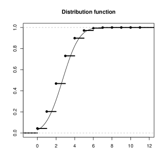
Fig. 5: Checking the convergence for $N=20$: First graph and its results.

The second graph has a different shape, as it corresponds to an adjacency matrix with band structure. The graph and the two plots of the results are presented in Figure 6.

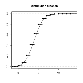
Fig. 6: Checking the convergence for $N=20$: Second graph and its results.

For the third graph analyzed here, we present only the results. The graph has been constructed with $N(N-1)/4=95$ edges randomly chosen among the $190$ edges of the complete graph with uniform probability. The results are shown in Figure 7.

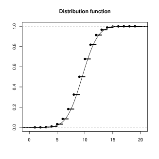
Fig. 7: Checking the convergence for $N=20$: The results for the third graph.

4 The mp-chart of the complement graph

In the literature, the complement of a graph $G=(V,E)$ is a graph on the same vertex set $V$ and the set of edges $V^{2}\setminus E$. Since our starting graph has no loop $(e,e)$, this forces $G^{c}$ to contain all of them. To avoid this problem we give a different definition of complement graph, more useful for our purposes.

Definition 24.

Given a graph $G=(V,E)$, its complement graph $G^{c}$ is a graph on the same vertex set $V$ and the set of edges $(V^{2}\setminus\Delta)\setminus E$, where $\Delta\subset E^{2}$ is the diagonal set, i.e. $\Delta=\{(v,v):v\in V\}$.

Remark 25.

From the previous definition, we notice that, if $G$ and $G^{c}$ have respectively $\ell_{G}$ and $\ell_{G^{c}}$ edges, then $\ell_{G}+\ell_{G^{c}}={N(N-1)}/{2}$.

As mentioned in Section 3, there are some nice properties linking the mp-chart $H_{G}$ of a graph $G$ with the mp-chart of its complement $G^{c}$. To study these connections, we start with a preliminary lemma.

Lemma 26.

Let $G$ be a graph with $N$ vertices. Denote by $T_{ij}^{c}$ the scalar product between the $i$-th row and $j$-th column in the adjacency matrix of $G^{c}$. The following formula relates the quantities $T_{ij}^{c}$ and $T_{ij}$:

$$T^{c}_{ij}=T_{ij}+N-2-d_{i}-d_{j}+<r_{i},E_{j}>+<r_{j},E_{i}>.$$ (13)

where the $E_{i}$’s are the vectors in the canonical basis of ${\mathbb{R}}^{N}$.

Proof.

Define the vector

$$v_{ij}=r_{i}-r_{j}-<r_{i}-r_{j},E_{i}>E_{i}-<r_{i}-r_{j},E_{j}>E_{j}$$ (14)

Since $<r_{i}-r_{j},E_{i}>=<r_{i},E_{i}>-<r_{j},E_{i}>$ and $<r_{t},E_{t}>=0$ (in fact, the $t$-th coordinate of $r_{t}$ is zero, while $E_{t}$ has a $1$ in the $t$-th coordinate and $0$ elsewhere), we can write

$$v_{ij}=r_{i}-r_{j}+<r_{j},E_{i}>E_{i}-<r_{i},E_{j}>E_{j}$$

The scalar product $<v_{ij},v_{ij}>$ measures the number of positions, out of the diagonal, where $r_{i}$ and $r_{j}$ are different. Thus, if we denote by $T^{c}_{ij}$ the scalar product of the corresponding lines, $r_{i}^{c}$, $r_{j}^{c}$ in the complement graph, one has

$$T^{c}_{ij}=N-2-T_{ij}-<v_{ij},v_{ij}>.$$ (15)

Now, we substitute in the previous formula the expression of $v_{ij}$ given in (14), and we obtain:

$$\begin{split}T^{c}_{ij}&=N-2-T_{ij}-<v_{ij},v_{ij}>=N-2-T_{ij}-\\ &-<r_{i}-r_{j}+<r_{j},E_{i}>E_{i}-<r_{i},E_{j}>E_{j},r_{i}-r_{j}+<r_{j},E_{i}>E_{i}-<r_{i},E_{j}>E_{j}>.\end{split}$$

Noting that $<r_{t},r_{t}>=d_{t}$ and $<r_{i},r_{j}>=<r_{j},r_{i}>=T_{ij}$, a straightforward computation leads to

$$T^{c}_{ij}=T_{ij}+N-2-d_{i}-d_{j}+<r_{i},E_{j}>^{2}+<r_{j},E_{i}>^{2}.$$

Since, for all $i$,$j$, with $i\not=j$, the value of $<r_{i},E_{j}>$ can be either $0$ or $1$, we can remove the squares from the previous formula, leading to Equation (13). ∎

Theorem 27.

Given a graph $G$ with $N$ vertices,

• $\mathbb{E}(H_{G^{c}})=N-1-\mathbb{E}(H_{G})$;

• $\mathbb{V}(H_{G^{c}})=\mathbb{V}(H_{G})+1-2{\mathbb{E}(H_{G})}/{(N-1)}$.

Proof.

To prove part $(a)$, it is enough to use Theorem 17 and Remark 25. One has

$$\mathbb{E}(H_{G^{c}})=\frac{2\ell_{G^{c}}}{N}=\frac{N(N-1)-2\ell_{G}}{N}=N-1-\mathbb{E}(H_{G})\,.$$

To prove part $(b)$, we apply Theorem 19 to the graph $G^{c}$. Therefore we have:

$$\mathbb{V}(H_{G^{c}})=\sum_{i=1}^{N}\frac{d_{i}^{c}(N-d_{i}^{c})}{N^{2}}+\sum_{\begin{subarray}{c}i,j=1\\ i\neq j\end{subarray}}^{N}\frac{d_{i}^{c}d_{j}^{c}-NT^{c}_{i,j}}{N^{2}(N-1)}\,.$$

The degree $d_{i}^{c}$ of a vertex in the complement graph is given by $d_{i}^{c}=N-1-d_{i}$. Using also Lemma 26 one can write $\mathbb{V}(H_{G^{c}})$ as

$$\begin{split}&\mathbb{V}(H_{G^{c}})=\sum_{i=1}^{N}\frac{(N-1-d_{i})(d_{i}+1)}{N^{2}}+\\ &+\sum_{\begin{subarray}{c}i,j=1\\ i\neq j\end{subarray}}^{N}\frac{(N-1-d_{i})(N-1-d_{j})-N(T_{ij}+N-2-d_{i}-d_{j}+<r_{i},E_{j}>+<r_{j},E_{i}>)}{N^{2}(N-1)}\end{split}$$ (16)

The first sum in formula (16) can be written as

$$\sum_{i=1}^{N}\frac{(d_{i})(N-d_{i})}{N^{2}}+\sum_{i=1}^{N}\frac{(N-1-2d_{i})}{N^{2}}\,,$$

where an easy computation shows that

$$\sum_{i=1}^{N}\frac{(N-1-2d_{i})}{N^{2}}=\frac{N-1}{N}-\frac{4\ell_{G}}{N^{2}}\,.$$

About the second sum in formula (16), we observe that each term can be expressed as

$$\begin{split}&\frac{(N-1-d_{i})(N-1-d_{j})-N(T_{ij}+N-2-d_{i}-d_{j}+<r_{i},E_{j}>+<r_{j},E_{i}>)}{N^{2}(N-1)}=\\ &=\frac{d_{i}d_{j}-NT_{i,j}+d_{i}+d_{j}+1-N(<r_{i},E_{j}>+<r_{j},E_{i}>)}{N^{2}(N-1)}\,.\end{split}$$

Since

$$\sum_{\begin{subarray}{c}i,j=1\\ i\neq j\end{subarray}}^{N}<r_{i},E_{j}>+<r_{j},E_{i}>)=4\ell_{G}\ \mbox{ and }\ \sum_{\begin{subarray}{c}i,j=1\\ i\neq j\end{subarray}}^{N}(d_{i}+d_{j})=4\ell_{G}(N-1)$$

the second sum becomes

$$\sum_{\begin{subarray}{c}i,j=1\\ i\neq j\end{subarray}}^{N}\frac{d_{i}d_{j}-NT_{i,j}}{N^{2}(N-1)}+\frac{4(N-1)\ell_{G}-N(N-1)-4N\ell_{G}}{N^{2}(N-1)}\,.$$

Thus, we obtain

$$\mathbb{V}(H_{G^{c}})=\mathbb{V}(H_{G})+1-\frac{4\ell_{G}}{N(N-1)}$$

and, considering Theorem 17, the formula in (b) follows. ∎

Some major remarks on the Theorem above are now in order.

Remark 28.

As a first trivial example, we consider the limit situation of an empty graph. Let $G$ be the empty graph. Its mp-chart has $\mathbb{E}(H_{G})=\mathbb{V}(H_{G})=0$. In this case $G^{c}$ is the complete graph with ${N(N-1)}/{2}$ edges and, by Theorem 27 part (b), one has $\mathbb{V}(H_{G^{c}})=1$. This can be verified also by direct computation. As a matter of fact, the adjacency matrix of $G^{c}$ consists of non-zero entries out of the diagonal. Thus $d_{i}^{c}=N-1$ for all $i$ and $T_{ij}^{c}=N-2$ for all $i$,$j$, with $i\not=j$. Hence

$$\mathbb{V}(H_{G})=\sum_{i=1}^{N}\frac{d_{i}(N-d_{i})}{N^{2}}+\sum_{\begin{subarray}{c}i,j=1\\ i\neq j\end{subarray}}^{N}\frac{d_{i}d_{j}-NT_{i,j}}{N^{2}(N-1)}=\frac{N-1}{N}+\frac{(N-1)^{2}-N(N-2)}{N^{2}(N-1)}=1\,.$$

These computations show that the variance of the mp-chart of a complete graph is invariant on the number of vertices.

Remark 29.

Few straightforward algebraic calculations show that the difference ${\mathbb{V}}(H_{G^{c}})-{\mathbb{V}}(H_{G})$ lies between $-1$ and $1$. Therefore, under the hypotheses of Theorem 22, when $N$ goes to infinity we have that ${\mathbb{V}}(H_{G^{c}})\cong{\mathbb{V}}(H_{G})$. Intuitively, the difference between ${\mathbb{V}}(H_{G^{c}})$ and ${\mathbb{V}}(H_{G})$ depends on the diagonal entries which are forced to be zero in the adjacency matrix $A_{G^{c}}$. The effect of these entries vanishes when the size of the graph goes to infinity.

Remark 30.

Another interesting property follows from Theorem 27. First, notice that ${\mathbb{E}}(H_{G^{c}})={\mathbb{E}}(H_{G})$ implies that $G$ and $G^{c}$ have the same number of edges, namely $N(N-1)/4$. (This is not possible for all values of $N$). In such a case, $H_{G^{c}}$ and $H_{G}$ are forced to have the same variance, no matter how is complicated the graph $G$.

The computation of the whole mp-chart of the complement graph $G^{c}$ from the mp-graph of $G$ is less easy. Given a graph G, we build a $(N+1)\times(N+1)-$matrix $M_{G}$, indexed, both on rows and columns, by $\{0,\dots,N\}$, an defined as follows. The entry $(M_{G})_{i,j}$ is the number of permutations $\pi$ such that $\sum_{s=1}^{N}(A_{G})_{s,\pi(s)}=j$ and $\pi$ has $i$ diagonal elements (that is, $\pi(s)=s$ for $i$ elements).

Example 31.

Consider the graph $G$ with matrix

$$A_{G}=\begin{pmatrix}0&0&0&1\\ 0&0&1&0\\ 0&1&0&1\\ 1&0&1&0\end{pmatrix}\,.$$

The corresponding matrix $M_{G}$ is

$$M_{G}=\begin{pmatrix}1&2&3&2&1\\ 0&4&4&0&0\\ 3&0&3&0&0\\ 0&0&0&0&0\\ 1&0&0&0&0\end{pmatrix}\,.$$

The matrix $M_{G}$ allows the computation of both the mp-charts $H_{G}$ and $H_{G^{c}}$. Roughly speaking, to compute the mp-chart of $G$ is is enough to sum the columns of $M_{G}$, while to compute the mp-chart of $G^{c}$ we need to sum the entries of suitable diagonals of $M_{G}$. More precisely, the following relations hold true.

Proposition 32.

For a graph $G$, we have for all $j=1,\ldots,N$:

• The components of the mp-chart $H_{G}$ are:

  $$h_{G}(j)=\sum_{i=0}^{N}(M_{G})_{i,j}\,;$$

• The components of the mp-chart $H_{G^{c}}$ are:

  $$h_{G^{c}}(j)=\sum_{i=0}^{N-j}(M_{G})_{i,N-j-i}.$$

Proof.

The first relation follows by the definition of mp-chart, as the sum of entries in the $j$-th column of $M_{G}$ is the number of permutations with $j$ elements equal to $1$, that is $h_{G}(j)$.

To prove the second relation, it is enough to prove that for all $i$ and $j$ we have: $(M_{G^{c}})_{i,j}=(M_{G})_{i,N-j-i}$. Suppose that $\pi$ is such that $\sum_{s=1}^{N}(A_{G})_{s,\pi(s)}=j$ and $\pi$ has $i$ diagonal elements. When we consider $\pi$ on $A(G^{c})$, we have $A(G^{c})_{s,\pi(s)}=1$ for the $s$ such that $(A_{G})_{s,\pi(s)}=0$, except for the diagonal entries where we still have 0. Hence there are $N-j-i$ entries in $A(G^{c})$ such that $A(G^{c})_{s,\pi(s)}=1$. This completes the proof. ∎

Example 33.

Consider the complement graph $G^{c}$ of the graph $G$ in Example 31:

$$A_{G^{c}}=\begin{pmatrix}0&1&1&0\\ 1&0&0&1\\ 1&0&0&0\\ 0&1&0&0\end{pmatrix}\,.$$

Then

$$M_{G^{c}}=\begin{pmatrix}1&2&3&2&1\\ 0&4&4&0&0\\ 3&0&3&0&0\\ 0&0&0&0&0\\ 1&0&0&0&0\end{pmatrix}\,.$$

We notice that in this simple case $M_{G}=M_{G^{c}}$. This is due to the fact that $G$ and $G^{c}$, up to the labels of the vertices, are equivalent.

Remark 34.

In principle, the max-plus permanent of the complement graph $G^{c}$ can be computed from the matrix $M_{G}$. In fact, Proposition 32 shows that the mp-chart of the complement graph can be computed from the matrix $M_{G}$ by adding along suitable diagonals and the max-plus permanent is just the position of the last non-zero element of the mp-chart. However, as the matrix $M_{G}$ is not easy to compute for large graphs, this approach does not help in actual computations.

5 Future directions

The max-plus permanent and the mp-chart studied in this paper lead to several new questions. In fact, we have analyzed here only the case of undirected graph. Therefore, among the future directions of our research, there will be the extension of the definition of max-plus permanent and mp-chart for undirected and weighted graphs. Moreover, special classes of graphs may be studied, such as bipartite graphs, or fixed-degree graphs. In particular, fixed-degree graphs correspond to adjacency matrices with fixed margins and in that context algebraic and combinatorial methods have demonstrated already their potential.

Another possible research direction is strictly in graph theory. As a matter of fact it could be interesting to compare the mp-chart of a graph with other well-known descriptors of its complexity. In a recent work in progress the mp-chart is compared to matching polynomials. By several examples we know that there exist different graphs with the same mp-chart. We notice that, in all these cases, also the matching polynomials coincide. So a principal question would be: If two non-isomorphic graphs have the same mp-chart, then their matching polynomials are equal?

Finally, applications to large graphs, possibly through simulation techniques, will be investigated in order to use the tools presented in this paper to real data examples.

References

- [1] Réka Albert and Albert-László Barabási, Statistical mechanics of complex networks, Review of Modern Physics, 74 (2002), pp. 47–97.
- [2] Alexander Barvinok, Enumerating contingency tables via random permanents, Combin. Probab. Comput., 17 (2008), pp. 1–19.
- [3] , On the number of matrices and a random matrix with prescribed row and column sums and 0–1 entries, Adv. Math., 224 (2010), pp. 316–339.
- [4] Alexander Barvinok and John A. Hartigan, The number of graphs and a random graph with a given degree sequence. arXiv:1003.0356, 2010.
- [5] Norman Biggs, Algebraic Graph Theory, Cambridge University Press, New York, 2 ed., 1993.
- [6] Patrick Billingsley, Probability and Measure, John Wiley and Sons, New York, 3 ed., 1995.
- [7] Béla Bollobás, Modern Graph Theory, Springer-Verlag, New York, 1998.
- [8] , Random Graphs, Cambridge University Press, Cambridge, 2 ed., 2001.
- [9] Anirban Chakraborti, Ioane Muni Toke, Marco Patriarca, and Frederic Abergel, Econophysics: Empirical facts and agent-based models. arXiv:0909.1974, 2010.
- [10] Reinhard Diestel, Graph Theory, Springer, Heidelberg, 3 ed., 2005.
- [11] Rick Durrett, Random Graph Dynamics, Cambridge University Press, New York, 2007.
- [12] Ubaldo Garibaldi and Enrico Scalas, Finitary Probabilistic Methods in Econophysics, Cambridge University Press, Cambridge, UK, 2010.
- [13] Stéphane Gaubert and Frédéric Meunier, Carathéodory, Helly and the others in the max-plus world, Discrete Comput. Geom., 43 (2010), pp. 648–662.
- [14] Wassily Hoeffding, A combinatorial central limit theorem, Ann. Math. Statist., 22 (1951), pp. 558–566.
- [15] TaeHyun Hwang, Hugues Sicotte, Ze Tian, Baolin Wu, Jean-Pierre Kocher, Dennis A. Wigle, Vipin Kumar, and Rui Kuang, Robust efficient identification of biomarkers by classifying features on graphs, Bioinformatics, 24 (2008), pp. 2023–2029.
- [16] André A. Keller, Graph theory and economic models: from small to large size applications, Electronic Notes in Discrete Mathematics, 28 (2007), pp. 469–476.
- [17] Oliver Mason and Mark Verwoerd, Graph theory and networks in biology, IET Syst. Biol., 1 (2007), pp. 89–119.
- [18] Michael B. Monagan, Keith O. Geddes, K. Michael Heal, George Labahn, Stefan M. Vorkoetter, James McCarron, and Paul DeMarco, Maple 10 Programming Guide, Maplesoft, Waterloo ON, Canada, 2005.
- [19] R Development Core Team, R: A Language and Environment for Statistical Computing, R Foundation for Statistical Computing, Vienna, Austria, 2010. ISBN 3-900051-07-0.
- [20] Robert J. Serfling, Contribution to central limit theory for dependent variables, Ann. Math. Statist., 39 (1968), pp. 1158–1175.
- [21] Jonathan Silver, Eric Slud, and Keiji Takamoto, Statistical equilibrium wealth distributions in an exchange economy with stochastic preferences, Journal of Economic Theory, 106 (2002), pp. 417 –435.