An efficient implementation of the simulated annealing heuristic for the quadratic assignment problem

Abstract

The quadratic assignment problem (QAP) is one of the most difficult combinatorial optimization problems. One of the most powerful and commonly used heuristics to obtain approximations to the optimal solution of the QAP is simulated annealing (SA). We present an efficient implementation of the SA heuristic which performs more than 100 times faster then existing implementations for large problem sizes and a large number of SA iterations.

1 Introduction

Originally formulated by Koopmans and Beckmann (1957), the QAP is NP-hard and is considered to be one of the most difficult problems to be solved optimally. It was defined in the following context: A set of $N$ facilities are to be located at $N$ locations. The quantity of materials which flow between facilities $i$ and $j$ is $A_{ij}$ and the distance between locations $i$ and $j$ is $B_{ij}$. The problem is to assign to each location a single facility so as to minimize (or maximize) the cost

$$C=\sum_{i=1}^{N}\sum_{j=1}^{N}A_{ij}B_{p(i)p(j)},$$

where $p(i)$ represents the location to which $i$ is assigned.

The QAP formulation has since been applied to such diverse problems as the optimal assignment of classes to classrooms (Dickey and Hopkins, 1972), design of DNA microarrays (de Carvalho and Rahmann, 2006), cross species gene analysis (Kolar, et al., 2008), creation of hospital layouts (Elshafei, 1977), and assignment of components to locations on circuit boards (Steinberg, 1961).

In addition to being important in its own right, the QAP includes such other combinatorial optimization problems as the traveling salesman problem and graph partitioning as special cases.

There is an extensive literature that addresses the QAP and which is reviewed in Pardalos et al. (1994), Cela (1998), Anstreicher (2003), Loiola et al. (2007), James et al. (2009) and Burkhard et al. (2009). The QAP is exceedingly hard to solve optimally. With the exception of specially constructed cases, optimal algorithms have solved only relatively small instances with $N\leq 36$. Various heuristic approaches have been developed and applied to problems typically of size $N\approx 100$ or less. By contrast, a travelling salesman problem consisting of almost 25,000 towns in Sweden has been solved exactly (Applegate et al., 2007).

2 Background

The simulated annealing heuristic was first applied to the QAP by Burkhard and Rendl (1984) and was refined by Connolly (1990). The heuristic consists of swapping locations of two facilities. Proposed swaps can either be determined randomly or selected according to some sequential enumeration of all possible swaps. For each proposed swap, $\delta$, the change in cost for the potential swap, is calculated. The swap is made if $\delta$ is negative or if

$$e^{-\delta/T}>r,$$

where $T$ is an analog of temperature in physical systems that is slowly decreased according to a specified cooling schedule after each iteration and $r$ is a uniformly distributed random variable between 0 and 1. Randomly making moves which increase the cost is done to help escape from local minima.

In traditional implementations of the heuristic, the cost of making a swap is calculated from scratch when the swap is considered in order to determine if the swap should be made. The computational complexity of this calculation is $O(N)$; and if the SA run is composed of $I$ iterations, the complexity is $O(IN)$. We can write the time needed to execute $I$ iterations as

$$t_{trad}=c_{0}NI$$ (1)

where $c_{0}$ is a constant.

3 Approach

The approach we take here is to attempt to reduce the complexity by maintaining a matrix $\Delta$ of costs of each possible swap. This approach is motivated by the work of Taillard (1991), who applied a similar approach in the application of another heuristic, tabu search, to the QAP. Our $\Delta$-matrix approach is as follows:

• Initialize by creating a matrix $\Delta(p,u,v)$ containing the cost of swapping $u$ and $v$ for all $u$ and $v$, given a current assignment $p$.

• In each iteration, retrieve the cost $\Delta(p,r,s)$ of the proposed swap $(r,s)$.

• If the proposed swap is not made in a given iteration, go to (b).

• If the proposed swap is made in a given iteration, update $\Delta(p,u,v)$ to reflect the swap costs given the new permutation and go to (b).

• End after $I$ iterations.

The number of iterations in which a swap is performed divided by the total number of iterations is known as the acceptance rate $a(I)$.

The computational complexity of our approach has the following contributions.

• Retrieving the value of $\Delta(p,r,s)$ is of complexity $O(1)$.

• Assuming an acceptance rate, $a(I)$, the matrix $\Delta(p,r,s)$ must be updated $a(I)I$ times. The complexity of updating $\Delta(p,u,v)$ is $O(N^{2})$ as described in A.

Thus the complexity of our approach is

$$O(a(I)IN^{2})+O(I)$$

and we can write the CPU time of our approach $t_{\Delta}$ as

$$t_{\Delta}=c_{1}a(I)IN^{2}+c_{2}I$$

where $c_{1}$ and $c_{2}$ are constants. The performance improvement factor of our approach relative to the traditional approach is then

$$F\equiv\frac{t_{trad}}{t_{\Delta}}=\frac{c_{0}N}{c_{1}a(I)N^{2}+c_{2}}\to\frac{c_{0}}{c_{1}a(I)N}$$ (2)

for large $N$.

From Eq. (2) we see that the performance improvement is critically dependent on the acceptance rate $a(I)$. The constants $c_{0}$ and $c_{1}$ are independent of the problem instance, depending only on the SA implementation; for our implementation $c_{0}/c_{1}\approx 1/3$. For our approach to be beneficial, $F$ must have a value $>1$ and thus $a(I)$ must satisfy

$$a(I)\lesssim 1/3N.$$ (3)

It is useful to consider an instantaneous acceptance rate, $\tilde{a}(i)$, defined as the number of swaps performed in a window of iterations around iteration $i$ divided by the size of the window. Our numerical experiments indicate that $\tilde{a}(i)$ decreases with increasing $i$ as the SA run progresses (see B). For this reason, our program uses the traditional approach until an iteration at which $\tilde{a}(i)$ satisfies Eq. (3) and then begins using the more efficient $\Delta$-matrix approach.

For tabu search, a swap is made only after all possible $N(N-1)/2$ swaps are analyzed. Thus for tabu search, the acceptance rate, $a\sim 1/N^{2}$ and the performance improvement is of O(N). However, for simulated annealing $a$ is a function of the QAP instance and the number of iterations performed in a run. We know of no method of determining the acceptance rate a priori. Hence, in section 4.1 we measure $a(I)$ for different QAP instances and various values of $I$ to get a sense of the performance improvement we can expect.

4 Numerical Results

We perform numerical experiments on two classes of QAP instances: random instances and structured instances. The random instances are created in the same manner as the Taixxa instances (Taillard, 1991) in QAPLIB (Burkard et al. 1997); the $A$ and $B$ matrices are symmetric with zero diagonal; the matrix elements are chosen from independent uniform distributions. The structured instances are the Taixxxe instances created by Taillard ( Drezner et al., 2005) designed to model real-world applications which are difficult to treat using iterative heuristics such as SA; the instances are composed of matrices which are not random They are available at http://mistic.heig-vd .ch/taillard/.

All runs were performed on systems with Intel Xeon 2.4 GHz processors.

4.1 Acceptance Rate

To get an idea of the performance improvement we may expect, we measure the acceptance rate for a range of problem sizes and number of iterations for the problem instances discussed above. We use the c++ implementation written by Taillard that implements the SA heuristic of Connolly(1990). Taillard’s code is available at http://mistic.heig-vd .ch/taillard/ .

4.2 Random instances

In Fig. 1(a), we plot the acceptance rates $a(I)$ for the random instances versus the number of iterations performed for various problem sizes. We note that $a(I)$ decreases with increasing $I$ until reaching a minimum after which $a(I)$ increases slowly. The location of the minimum in $a(I)$ is dependent on $N$; the larger the problem size, the higher the number of iterations at which the minimum is reached. In B.1, we provide insights into this behavior.

We also note that for large numbers of iterations, $a(I)$ is lower for larger problem sizes. This is fortuitous because from Eq. (2) a lower value of $a(I)$ is needed to achieve the same performance improvement factor if $N$ is increased.

4.3 Structured instances

In Fig. 1(b), we plot the acceptance rate for the structured instances. The overall behavior is the same as for the random instances, but after the minimum is reached, $a(I)$ does not increase with $I$. In B.2, we provide explain this behavior. Also for instances of approximately the same size, $a(I)$ is higher for the structured instances than for the random instances. This implies that the performance improvement for the structured instances will not be as great as for the random instances.

4.4 Performance Improvement

We use the Taillard code as a base for our implementation described in Section 3. For the random instances, in Fig. 2 we plot CPU time vs the number of iterations for the traditional approach and for our $\Delta$-matrix approach. Note that the times for the traditional approach are linear with the number of iterations, consistent with Eq. (1). The $\Delta$-matrix approach results are coincident with those of the traditional approach until Eq. (3) is satisfied, at which point it is more efficient to use the $\Delta$ matrix. From this point on, the $\Delta$-matrix approach CPU times are lower than those of the traditional approach. Similar results hold for the structured instances as shown in Fig. 3.

In Fig. 4, we plot the measured performance improvement $t_{trad}/t_{\Delta}$ for random and structured instances. There is no performance improvement until the number of iterations $\sim 10^{6}$. This reflects the fact that below this number of iterations Eq. (3) does not hold and the traditional method is used. We see that the relative performance of the $\Delta$-matrix approach improves with increasing problem size, from which we can infer from Eq. (2) that the acceptance rate decreases faster than the problem size as the problem size increases.

5 Discussion and Summary

We develop an implementation of the simulated annealing heuristic for the quadratic assignment problem which runs significantly faster than the traditional implementation; the simulated annealing concept and algorithm for the QAP are unchanged. Our approach is motivated by the work of Taillard (1991) who took a similar approach in implementing tabu search for the quadratic assignment problem. That the technique has not been applied to SA until now may be due to the fact that it does not provide significant benefit unless a large number of iterations are applied to a large QAP instance; this is now possible with the improvement of computing capabilities over the last 20 years.

Being able to perform SA with a large number of iterations on large QAP instances is important because (a) many real world problems are significantly larger than the size of problems to which SA has been traditionally applied and (b) the quality of the SA solution improves as the number of iterations is increased (Paul, 2010). Also, in Paul (2010) it was shown that for high quality solutions, the performance of SA is superior to that of tabu search. The current work makes this finding stronger because of the improved performance of SA.

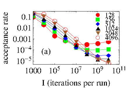
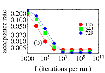
Figure 1: Acceptance rates for(a) random and (b) structured instances versus number of iterations.

$\begin{array}[]{c}\includegraphics[width=227.62204pt]{p128.eps}\includegraphics[width=227.62204pt]{p256.eps}\\ \includegraphics[width=227.62204pt]{p512.eps}\includegraphics[width=227.62204pt]{p1024.eps}\\ \includegraphics[width=227.62204pt]{p2048.eps}\includegraphics[width=227.62204pt]{p4096.eps}\\ \end{array}$

Figure 2: CPU time versus iterations for random instances for traditional implementation (circles) and efficient implementation (squares).

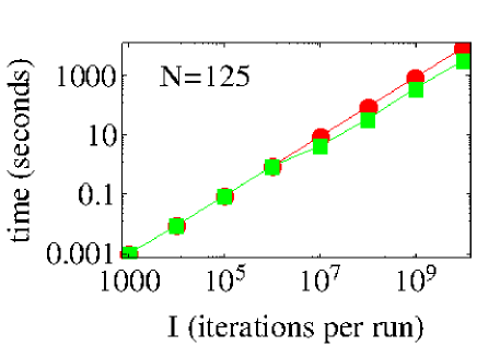
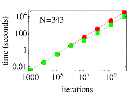
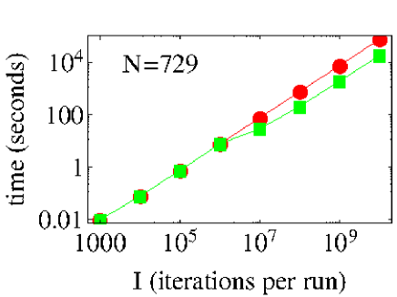
Figure 3: CPU time versus iterations for structured instances for traditional implementation (circles) and efficient implementation (squares).

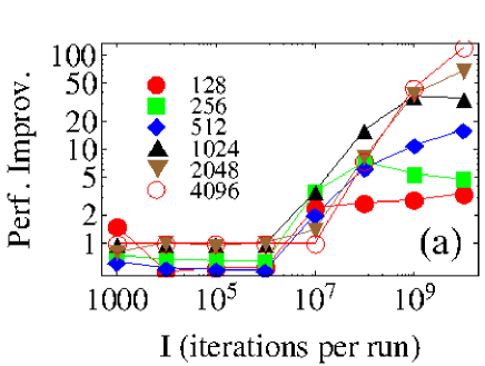
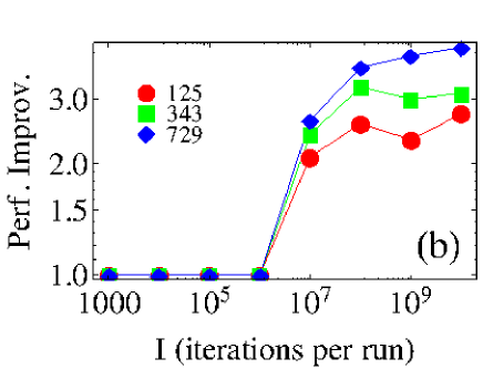
Figure 4: Performance improvement for (a) random instances and (b) structured instances.

Appendix A Complexity of $\Delta$-Matrix Update

Following Taillard (1991), starting from an assignment of facilities $p$ let the resulting assignment after swapping facilities $r$ and $s$ be $p^{\prime}$. That is:

$$p^{\prime}(k) = p(k)~{}~{}~{}~{}~{}k\neq r,s$$

$$p^{\prime}(r) = p(s)$$

$$p^{\prime}(s) = p(r).$$

For a symmetrical matrix with a null-diagonal, the cost $\Delta(p,r,s)$ of swapping $r$ and $s$ is:

$$\Delta(p,r,s) = \sum_{i=1}^{N}\sum_{j=1}^{N}(A_{i,j}B_{p(i),p(j)}-A_{i,j}B_{p^{\prime}(i),p^{\prime}(j)})$$

$$= 2\sum_{k\neq r,s}(A_{s,k}-A_{r,k})(B_{p(s),p(k)-B_{p(r)},p(k)}).$$

To calculate $\Delta(p^{\prime},u,v)$ for any $u$ and $v$ with complexity O(N) , we can use equation (LABEL:eqfull). For asymmetric matrices or matrices with non-null diagonals, a slightly more complicated version of Equation (LABEL:eqfull) also of complexity O(N) is given by Burkhard and Rendl (1984).

In the case that $u$ and $v$ are different from $r$ or $s$, we can calculate $\Delta(p^{\prime},u,v)$ with complexity $O(1)$ with

$$\Delta(p^{\prime},u,v)=\Delta(p,u,v)+2(A_{r,u}-A_{r,v}+A_{s,v}-A_{s,u})$$

$$\times(B_{p^{\prime}(s),p^{\prime}(u)}-B_{p^{\prime}(s),p^{\prime}(v)}+B_{p^{\prime}(r),p^{\prime}(v)}-B_{p^{\prime}(r),p^{\prime}(u)})$$

using the value $\Delta(p,u,v)$ calculated in the previous iteration. Since there are $O(N^{2})$ matrix entries with $u$ and $v$ different from $r$ or $s$, these contribute complexity $O(N^{2})$ to the $\Delta$ matrix update. There are $O(N)$ entries with $u$ and $v$ not different from $r$ or $s$ each of which requires the $O(N)$ calculation of Eq. (LABEL:eqfull). These entries thus also contribute complexity $O(N^{2})$ and the overall complexity of updating $\Delta$ is $O(N^{2})$.

Appendix B Acceptance rate behavior

Because the performance improvement depends critically on the acceptance rate as shown in Eq. (2), here we explore the behavior of the acceptance rate as shown in Fig. 1. In order to do this, we first provide more details of the cooling schedule of the SA algorithm (Connolly, 1990) and describe how an SA run progresses.

The details of the cooling schedule are as follows: At the start of each heuristic run, the temperature is set to a high value $T_{0}$. After each iteration, the temperature is reduced using the recursive relation

$$T=\frac{T}{1.0+\beta T}$$ (5)

where

$$\beta\equiv\frac{T_{0}-T_{f}}{IT_{0}T_{F}}.$$ (6)

to reach a desired final temperature $T_{f}$ when all iterations are exhausted. Note from Eq. (6) that the temperature decreases in smaller steps for larger $I$. The temperature decrease may end before $T_{f}$ is reached if a specified number, $Q$, of consecutive iterations in which no swap is performed is encountered. We denote the temperature at which this occurs as $T_{Q}$.

At the beginning of an SA run, the initial QAP configuration is random and there are relatively many moves which will result in a cost decrease. As the run progresses, the number of moves which will result in a lower cost decreases. Also as the run progresses, the decreasing temperature results in a lower frequency of swaps with a positive incremental cost $\delta$. Thus the instantaneous acceptance rate $\tilde{a}(i)$ (defined in Section 3) decreases as the run progresses. Eventually if the number of iterations $I$ specified for the run is large enough, the number of consecutive iterations in which a swap is not performed will exceed the specified limit $Q$ and the temperature and $\tilde{a}(i)$ will no longer decrease.

With this background we now discuss the behavior of the acceptance rates $a(I)$ shown in Fig. 1 for both the random and structured instances.

B.1 Random instances

To study the acceptance rate $a(I)$ at a more granular level, for various values of $I$, Fig. 1 plots the instantaneous acceptance rate $\tilde{a}(i)$ versus the iteration number $i$ for $N=128$; plots for other values of $N$ are similar. For $I\gtrsim 10^{6}$, the plots for each value of $I$ eventually reach constant values $a_{x}(I)$. The plots become constant at the iteration at which no swaps have been performed in the previous $Q$ iterations at which point the temperature is fixed at $T_{Q}$. We also note that the constant values $a_{x}(I)$ increase with increasing $I$. This behavior can be understood by plotting $T_{Q}$. For the random $N=128$ instance, in Fig. 2 we plot $T_{Q}$ as function of $I$ and note that $T_{Q}$ increases with increasing $I$. This reflects the fact that because of the the slower cooling for larger number of iterations, SA finds a deeper local minima from which it cannot escape easily at a higher temperatures for larger $I$. The increase in $a_{x}(I)$ as $I$ increases explains the increase in $a(I)$ for larger values of $I$ in Fig. 1 (a).

For $I\lesssim 10^{6}$, the plots in Fig. 1 terminate at lower and lower values as $I$ increases. This explains the initial decrease in the acceptance rate as a function of $I$ in Fig. 1(a). The plots do not reach a constant value and terminate at a higher value than plots with $I\gtrsim 10^{6}$. This occurs because despite the low temperatures at the end of run which inhibit cost-raising swaps, there are sufficient numbers of cost-reducing swaps to maintain a relatively high value of $\tilde{a}(i)$.

B.2 Structured instances

As with the random instances, in order to understand the behavior in Fig. 1(b) we must study the instantaneous acceptance rate $\tilde{a}(i)$. For various values of $I$, Fig. 3 plots $\tilde{a}(i)$ versus the $i$. As opposed to the random instances, all plots decrease monotonically and never level off to a constant value. This behavior is explained by the fact that for the structured instances studied, the limit $Q$ on the number of consecutive iterations in which no swap is made is never reached; there are always low cost swaps which can be made. The temperature always decreases to $T_{f}$ and as the temperature decreases $\tilde{a}(i)$ decreases. Because the plots in Fig. 3(b) for larger $I$ all scale with the number of iterations, the value reached by the plots in Fig. 1(b) remain constant for large $I$.

Similar to the behavior for the random instances and for the same reason, for $I\lesssim 10^{6}$, the $\tilde{a}(i)$ plots terminate at a higher value than plots with $I\gtrsim 10^{6}$. As with the random instances, this explains the initial decrease in the acceptance rate as a function of $I$ in Fig. 1( b).

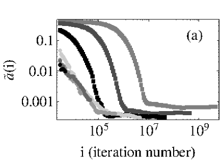
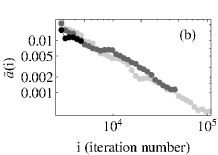
Figure 1: (a) For the random $N=128$ instance, instantaneous acceptance rate vs iteration number $i$ for (from left to right) $I=10^{4},10^{5},10^{6},10^{7},10^{8},10^{9}$ and $10^{10}$. (b) Detail for $I=10^{4}$ (black), $10^{5}$ (medium gray), $10^{6}$ (light gray).

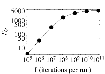
Figure 2: For the random $N=128$ instance, temperature $T_{Q}$ versus number of iterations, I, specified for run. $T_{Q}$ is the temperature at which  the specified number of consecutive iterations in which a swap is not performed is encountered. The temperature is not lowered below this value.

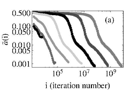
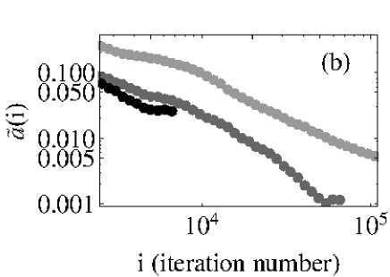
Figure 3: (a) For the structured $N=125$ instance, instantaneous acceptance rate vs iteration number $i$ for (from left to right) $I=10^{4},10^{5},10^{6},10^{7},10^{8},10^{9}$ and $10^{10}$. (b) Detail for $i=10^{4},10^{5}$ and $10^{6}$.

Appendix C Supplementary material

The c++ program which implements the SA heuristic described in this article can be found, in the online version, at doi:xxxxxx.

References

• Anstreicher, K., 2003. Recent advances in the solution of quadratic assignment problems. Mathematical Programming 97, 27-42.

• Applegate, D.L. Bixby, R.E, Chvatal, V., Cook, W.J., 2007. The Traveling Salesman Problem: A Computational Study, Princeton University Press.

• Burkard, R.E., Cela, E., Karish,S. E., Rendl, F., 1997. QAPLIB - A Quadratic Assignment Problem Library. J. Global Optim. 10 (1997) 391-403; http://www.seas.upenn.edu/qaplib/

• Burkard, R. E., Dell’Amico, M. & Martello, S., 2009. Assignment Problems, SIAM Philadelphia.

• Burkard R. E., Rendl, F., 1984. A thermodynamically motivated simulation procedure for combinatorial optimization problems. EJOR 17, 169-174,

• Cela E., 1998. The Quadratic Assignment Problem: Theory and Algorithms. Kluwer, Boston, MA.

• Connolly, D. T., 1990. An improved annealing scheme for the QAP, EJOR 46 93-100.

• de Carvalho Jr., S. A., Rahmann, S., 2006. Microarray layout as a quadratic assignment problem. In Hudson, D. et al., eds. German Conference on Bioinformatics (GCB), Lecture Notes in Infomatics. P-83, 11–20 .

• Dickey, J., Hopkins, J. 1972. Campus building arrangement using TOPAZ. Transportation Res. 6, 59–68.

• Drezner, Z., Hahn,P.M., Taillard È. D., 2005. Recent Advances for the quadratic assignment problem with special emphasis on instances that are difficult for meta-heuristic methods. Annals of Operations Research 139, 65-94.

• Elshafei, A. N, 1977. Hospital layout as a quadratic assignment problem. Operations Res. Quarterly 28, 167–179.

• James, T., Rego, C., Glover, F., 2009a. Multistart Tabu Search and Diversification Strategies for the Quadratic Assignment Problem. IEEE Tran. on Systems, Man, and Cybernetics PART A: SYSTEMS AND HUMANS 39, 579-596.

• Kolář, M., Lässig, M., Berg, J., 2008. From protein interactions to functional annotation: Graph alignment in Herpes. BMC Systems Biol. 2, Article 90.

• Koopmans T., Beckmann, M., 1957. Assignment problems and the location of economic activities. Econometrica 25, 53-76.

• Loiola,E.M., de Abreu, N.M.M., Boaventuro-Netto, P.O., Hahn, P., Querido, T., 2007. A survey for the quadratic assignment problem. European Journal of Operational Research 176, 657-690.

• Pardalos, P. M., Pitsoulis, L. S., Resende, M. G. C., 1997. Algorithm 769: Fortran subroutines for approximate solution of sparse quadratic assignment problems using GRASP. ACM Transactions on Mathematical Software (TOMS) 23, 196-208.

• Paul, G., 2010. Comparative performance of tabu search and simulated annealing heuristics for the quadratic assignment problem. Operations Research Letters 38 577-581

• Steinberg, L., 1961. The backboard wiring problem: A placement algorithm. SIAM Rev. 3, 37-50.

• Taillard, E., 1991. Robust taboo search for the quadratic assignment problem. Parallel Computing 17, 443-455; code available at:http://mistic.heig-vd.ch/taillard/codes.dir/tabou_qap.cpp.