The contribution of star-forming galaxies to fluctuations in the cosmic background light.
Abstract
Star-forming galaxies which are too faint to be detected individually produce intensity fluctuations in the cosmic background light. This contribution needs to be taken into account as a foreground when using the primordial signal to constrain cosmological parameters. The extragalactic fluctuations are also interesting in their own right as they depend on the star formation history of the Universe and the way in which this connects with the formation of cosmic structure. We present a new framework which allows us to predict the occupation of dark matter haloes by star-forming galaxies and uses this information, in conjunction with an N-body simulation of structure formation, to predict the power spectrum of intensity fluctuations in the infrared background. We compute the emission from galaxies at far-infrared, millimetre and radio wavelengths. Our method gives accurate predictions for the clustering of galaxies both for the one halo and two halo terms. We illustrate our new framework using a previously published model which reproduces the number counts and redshift distribution of galaxies selected by their emission at m. Without adjusting any of the model parameters, the predictions show encouraging agreement at high frequencies and on small angular scales with recent estimates of the extragalactic fluctuations in the background made from early data analysed by the Planck Collaboration. There are, however, substantial discrepancies between the model predictions and observations on large angular scales and at low frequencies, which illustrates the usefulness of the intensity fluctuations as a constraint on galaxy formation models.
keywords:
galaxy clustering, PlanckThe contribution of star-forming galaxies to fluctuations in the cosmic background light.
1 Introduction
The cosmic background light (CBL) is a rich source of information about the conditions in the early universe and the subsequent growth of galaxies and of structure in the dark matter. Accurate measurements of the power spectrum of temperature anisotropies in the primordial component have led to tight constraints being placed on the values of the basic cosmological parameters (e.g. Komatsu et al. 2011). Other contributions to the CBL include Galactic cirrus, the thermal and kinetic Sunyaev-Zel’dovich effects and extragalactic sources such as star-forming galaxies (SFGs) and active radio galaxies (see e.g. Figure 2 of Dunkley et al. 2011). Correlated fluctuations in the CBL due to SFGs depend on the number of sources and their clustering, which in turn is sensitive to the variation in the efficiency of star formation with dark matter halo mass. The extragalactic contribution to the CBL may be viewed either as a nuisance to be removed statistically in order to get to the primordial CBL signal, or as an interesting quantity in its own right as a challenge to models of the clustering of galaxies and their emission in the infra-red, millimetre and radio ranges of the electromagnetic spectrum.
A small fraction, around 10-20%, of the extragalactic background light has been resolved into galaxies at far-infrared and millimetre wavelengths (Bethermin et al. 2010; Oliver et al. 2011). Fluctuations in the intensity of the unresolved CBL have been discovered recently (Grossan & Smoot 2007; Lagache et al. 2007; Viero et al. 2009; Hall et al. 2010; the Planck Collaboration 2011b; Penin et al. 2012a). These fluctuations have two sources: the shot noise arising from sampling a discrete number of unresolved galaxies within the telescope beam and the intrinsic clustering of the galaxies. In an early analysis of six regions of low Galactic extinction covering square degrees, the Planck Collaboration (2011b) have cleaned the temperature anisotropy maps to leave only the extragalactic fluctuations in the CBL. This is done by using the lowest frequency Planck map to remove the cosmological signal (we shall see later that fluctuations due to the clustering of extragalactic sources are negligible at low frequencies) and exploiting neutral hydrogen observations as a tracer of dust to further reduce the contribution from Galactic emission. (For an overview of the Planck mission, see the Planck Collaboration 2011a.)
A variety of models have been developed to interpret the measured power spectrum of fluctuations in the intensity of the CBL. These models have predominantly used empirical spectral energy distributions (e.g. Lagache et al. 2003, 2007). Simple analytic models have been assumed for the clustering of galaxies such as a linear bias factor relative to the clustering of the dark matter (e.g. Knox et al. 2001; Fernandez-Conde et al. 2008; Hall et al. 2010) or the halo occupation distribution (HOD) formalism (Amblard & Cooray 2007; Viero et al. 2009; Shang et al. 2011; Penin et al. 2012b). Righi et al. (2008) presented a calculation based on the mergers of dark matter haloes and a simple dust evolution model. Seghal et al. (2010) assumed that the number of infra-red sources scaled with halo mass to compute the two halo clustering, without calculating a one halo contribution. Negrello et al. (2007) combined the model of Granato et al. (2004) for the evolution of the spheroid population with a phenomenological model for the evolution of starbursts, normal late-type spirals and radio galaxies. These authors assumed a linear bias to model the clustering of galaxies. The Planck Collaboration (2011b) have used their measurements of the CBL fluctuations to rule out a linear bias model that is constrained to match the observed number counts of galaxies, arguing that accurate small-scale clustering predictions are critical to match the observations.
In this paper we present a new approach for computing the contribution of SFGs to the intensity fluctuations in the CBL, with two important improvements over previous theoretical models. First, we make an ab initio calculation of the spectral energy distributions of a large sample of galaxies, using a self-consistent treatment of the extinction of starlight by dust and the reprocessing of the absorbed energy to longer wavelengths. We also compute the radio emission from star-forming galaxies (Condon 1992; Bressan, Silva & Granato 2002). Second, we combine the predictions for the properties of the galaxy population with a high resolution, large volume N-body simulation of the clustering of matter in the Universe. This allows us to accurately model the clustering of galaxies over a wide range of pair separations, including the highly nonlinear regime corresponding to scales within an individual dark matter halo. Empirical models suffer from the obvious drawback that the bulk of the galaxies responsible for the extragalactic background have not yet been observed, which makes the calibration of this class of model uncertain. Also, without the context of a model for structure formation, any assumptions about the clustering of the galaxies are decoupled from their abundance (e.g. as in the calculation by Xia et al. 2012).
The first step in our calculation is to generate predictions for the star formation histories of a representative sample of galaxies, using the semi-analytical galaxy formation code, GALFORM (Cole et al. 2000; Baugh et al. 2005). The star formation and metal enrichment histories, along with the size of the disc and bulge components are input to the spectro-photometric code GRASIL (Silva et al. 1998). GRASIL is used to compute the spectral energy distribution of each galaxy, using a radiative transfer calculation in a two-phase dust medium (Granato et al. 2000). We describe how the hybrid GALFORM plus GRASIL code is implanted into a large-volume, high resolution N-body simulation of the clustering of the dark matter to add information about the spatial distribution of galaxies. This allows an accurate treatment of the one-halo term and of the nonlinear component of the two-halo term.
The content of the paper is as follows. In Section 2 we give a brief overview of the GALFORM and GRASIL models before explaining how we populate an N-body simulation with model galaxies. In Section 2.3 we set out the calculation of the angular correlation function of flux. The results of the paper are presented in Section 3 and the summary in Section 4. The appendix discusses the sensitivity of the model predictions to the finite resolution of the N-body simulation.
2 Theoretical background
In this section we introduce the galaxy formation model used and outline the theoretical concepts needed in the paper. We give a brief overview of the semi-analytical galaxy formation model and explain how the emission from dust and at radio wavelengths is computed in Section 2.1. The implementation of this model in an N-body simulation is described in Section 2.2. In Section 2.3 we set out the equations describing how the clustering of intensity fluctuations due to extragalactic sources is computed from the predictions of the galaxy formation model.
| LFI | LFI | LFI | HFI | HFI | HFI | HFI | HFI | HFI | |
|---|---|---|---|---|---|---|---|---|---|
| Frequency (GHz) | 30 | 44 | 70 | 100 | 143 | 217 | 353 | 545 | 857 |
| Wavelength (mm) | 10 | 6.81 | 4.29 | 3.0 | 2.1 | 1.38 | 0.85 | 0.55 | 0.35 |
| Flux limit (Jy) | 0.23 | 0.25 | 0.24 | 0.25 | 0.25 | 0.16 | 0.33 | 0.54 | 0.71 |
| Angular resolution (arcmin) | 33 | 24 | 14 | 9.5 | 7.1 | 5.0 | 5.0 | 5.0 | 5.0 |
2.1 The hybrid galaxy formation model
We use a hybrid model consisting of the GALFORM semi-analytical galaxy formation code (Sec 2.1.1) and the GRASIL spectrophotometric code (Sec 2.1.2).
2.1.1 The GALFORM galaxy formation model
The formation and evolution of galaxies within the CDM cosmology is predicted using the semi-analytical model GALFORM (Cole et al. 2000). The main processes modelled include: (1) the formation of dark matter haloes by mergers and the accretion of smaller haloes, (2) the growth of galactic discs following the shock-heating and radiative cooling of gas inside dark matter haloes, (3) star formation in galactic discs, (4) the reheating and ejection of gas by supernovae, (5) the prevention of gas cooling in low circular velocity haloes due to the photoionization of the intergalactic medium, (6) the loss of galaxy orbital energy through dynamical friction, (7) the subsequent merger between galaxies, which may be accompanied by a burst of star formation and (8) chemical evolution of the stars and gas. By following these processes, GALFORM predicts the star formation history of each galaxy (see Baugh 2006 for a review). The code can be run quickly for a representative sample of dark matter haloes, making it ideal for generating predictions for number counts and to populate large volumes to predict galaxy clustering.
The galaxy formation model we use in this paper is that of Baugh et al. (2005; see also Lacey et al. 2010). This model reproduces the observed number counts and redshift distribution of galaxies at m, and also the luminosity function of Lyman break galaxies (see Lacey et al. 2011). (Note that the more recent model of Bower et al. 2006 does not enjoy these successes, and so is not used in this paper.) The background cosmology is a spatially flat CDM model (see later for the values of the cosmological parameters). The merger histories of the dark matter haloes are generated using an improved Monte Carlo technique that has been calibrated against merger trees extracted from an N-body simulation (Parkinson, Helly & Cole 2008).
The model follows two modes of star formation, a “quiescent” mode which takes place in galactic discs and a “burst” mode which is triggered by major and minor galaxy mergers. Mergers are classified according to the ratio of the mass of the merging satellite, , to that of the central galaxy, . If (where is a model parameter) then the merger is defined as a major merger. In this case, any cold gas in the two galaxies takes part in a starburst which adds stars to the spheroid. Minor mergers which have mass ratios in the range and where the primary is also gas rich, with are also assumed to trigger starbursts. In the Baugh et al. model the parameter values were set to , and . Different stellar initial mass functions (IMF) are adopted in the two modes of star formation. Quiescent star formation is assumed to take place with a solar neighbourhood IMF (Kennicutt 1983). Bursts of star formation are assumed to form stars with a top heavy IMF. Baugh et al. (2005) argued that the adoption of a top heavy IMF in bursts is necessary to reproduce the observed number counts and redshift distributions of the faint sub-mm galaxies, whilst at the same time reproducing the properties of the local galaxy population.
2.1.2 The GRASIL spectrophotometric code
The frequencies sampled by the Planck Low Frequency Instrument (LFI; the Planck Collaboration 2011c) and High Frequency Instrument (HFI; the Planck Collaboration 2011d) are listed in Table 1. At these frequencies (corresponding to wavelengths -mm) we assume that the contribution from galaxies is dominated by star-forming galaxies through dust heated by stars and radio emission resulting from gas ionized by stars and synchrotron radiation from relativistic electrons accelerated in supernova remnant shockwaves. We do not attempt to model the contribution to the CBL of active galactic nuclei or galaxies in which the radio emission is powered by accretion onto a central black hole. To predict the emission from model galaxies at these frequencies we use the GRASIL spectrophotometric code (Silva et al. 1998; Bressan et al. 2002). GRASIL computes the emission from the composite stellar population of the galaxy, using theoretical models of stellar evolution and stellar atmospheres. The interaction of the starlight with dust is followed with a radiative transfer calculation which assumes a two-phase dust medium, and gives the distribution of dust temperatures within each galaxy using a detailed grain model. The output from GRASIL is the galaxy SED from the far-UV to the radio (wavelengths 0.01 m ). The main features of the hybrid GALFORM-GRASIL model are described in Lacey et al. (2010; see also Granato et al. 2000).
2.2 Populating an N-body simulation with galaxies
We combine the hybrid GALFORM-GRASIL galaxy formation model with a high resolution N-body simulation of the clustering of matter. This allows us to make accurate predictions for the clustering of galaxies selected by their emission at infrared, millimetre and radio wavelengths. In particular the small-scale clustering measured in the simulation can be significantly different in practice from simple analytical expectations based on linear perturbation theory (as shown, for example, by Benson et al. 2000). We shall see later that for some frequencies, the clustering of galaxy pairs within the same dark matter halo is important for the power spectrum of the microwave background intensity fluctuations on the angular scales probed by Planck.
We now describe how galaxies are implanted into an N-body simulation. Our starting point is a set of model galaxies generated using the hybrid GALFORM plus GRASIL code set in the concordance CDM cosmology, which we refer to as the MCGAL catalogue. The end point is a galaxy catalogue implanted in the Millennium Simulation of Springel et al. (2005), an N-body simulation of a cosmologically representative volume. We denote this as the MILLGAL catalogue. Some minor complications arise because the cosmology adopted in our original calculation is not quite the same as that of the N-body simulation; this issue is dealt with in step 2 below. The most accurate calculation of galaxy clustering is made using the MILLGAL catalogue, so we focus on this model in the main paper. In some instances we show predictions made using both versions of the model to illustrate regimes in which the MILLGAL predictions are superior. The MILLGAL calculation has a finite resolution; as we show in the Appendix, this does not affect our results.
The MCGAL catalogue is constructed by sampling galaxies according to their stellar mass from a much larger catalogue of galaxies. This larger catalogue is generated from halo merger histories generated using a Monte Carlo method (Cole et al. 2000; Parkinson et al. 2008). Star formation histories are extracted for the selected galaxies, which are then input to GRASIL, along with the predicted dust masses and sizes of the disc and bulge components, to compute the galaxy SED. For each galaxy we have the stellar mass, host halo mass, a weight based on the halo number density and on the sampling rate as a function of stellar mass, and the galaxy SED. Due to the computational expense of generating the MCGAL catalogue, and its similarity with the MILLGAL catalogue which we wish to build, we have devised the following scheme to take advantage of the availability of this calculation, rather than making a new calculation based on star formation histories extracted directly from galaxies in the Millennium simulation.
The steps followed to populate the Millennium simulation with galaxies starting from the MCGAL catalogue are as follows:
-
(1)
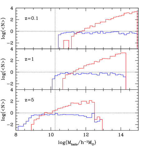
Construct the halo occupation distribution (HOD) of galaxies. GALFORM predicts how many galaxies are contained within each dark matter halo. The HOD quantifies the mean number of galaxies per halo as a function of the halo mass (Benson et al. 2000; Peacock & Smith 2000; Berlind & Weinberg 2002). Fig. 1 shows the HOD of galaxies in the MCGAL catalogue at three different redshifts. We plot the HOD for central (blue line) and satellite (red line) galaxies separately. Fig. 1 shows that the HODs of central galaxies in the MCGAL catalogue are approximately step functions. The shape of the satellite galaxy HOD is close to a power law in halo mass. The lowest mass dark matter halo which appears in the MCGAL HODs varies with redshift. The halo mass grid used in this calculation is defined at each redshift in order to sample haloes with a representative range of abundances. At , the lowest mass halo considered is nearly the same as the lowest mass halo which can be resolved in the Millennium simulation (, which is shown by the vertical dotted line in Fig. 1). The lowest mass dark matter halo in the Millennium simulation is the same at all redshifts. We cannot transplant galaxies from the MCGAL catalogue which reside in haloes below the mass resolution of the Millennium. We test the sensitivity of our predictions to this limitation of the N-body catalogue in the Appendix.
-
(2)
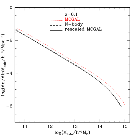
Match the halo mass function between the cosmologies used. The MCGAL catalogue, for historical reasons, assumes a slightly different cosmology to that adopted in the Millennium simulation. The Millennium cosmology is based on the first year of WMAP observations111The cosmological parameters in the Millennium are: matter density , cosmological constant , Hubble constant , primordial scalar spectral index , baryon density and fluctuation amplitude . The parameters in the MCGAL case are , , , , , and (Baugh et al. 2005).. At a given mass, the number density of haloes is slightly different in the two cosmologies. The GALFORM-GRASIL code is computationally expensive to run, which prohibits running the calculation again in the Millennium cosmology. A re-run would also require some retuning of the galaxy formation parameters. To transplant the galaxies from the halo population in one cosmology to that in the other cosmology, we instead chose to relabel the halo masses in the MCGAL model to force a match with the Millennium simulation mass function. Fig. 2 shows the halo mass functions in the original MCGAL calculation (red dotted line) and in the N-body simulation (black dashed line), along with the rescaled MCGAL halo mass function (black solid line) at . To match the halo mass functions at we reduce the halo mass globally in the MCGAL catalogue by a factor of . The halo mass function of the rescaled MCGAL catalogue and that of Millennium simulation agree to better than 5% over four decades in halo mass. We apply the same scheme to other redshifts and find that it works equally well, but with slightly different scaling factors. The small difference between the halo mass functions in the two cosmologies supports our decision not to rerun the GALFORM-GRASIL calculation in the cosmology of the Millennium simulation.
-
(3)
Place galaxies in the N-body simulation. We generate the MILLGAL catalogue of galaxies using the MCGAL HOD with halo masses rescaled, as explained in Step 2. The central galaxy is placed at the centre of mass of the halo. In the case of halo masses for which the HOD specifies , a fraction of the haloes of this mass are populated with a single galaxy at random with a probability . The number of satellite galaxies in a given halo mass is assumed to have a Poisson distribution for , with the mean number of satellite galaxies given by the HOD. Satellite galaxies are assigned to randomly selected dark matter particles which are part of the friends-of-friends halo.
2.3 Calculation of the angular power spectrum of intensity fluctuations
In this subsection we give the theoretical background to the calculation of the angular power spectrum of the intensity fluctuations of galaxies. The discussion is split into three parts: §2.3.1 The calculation of the angular correlation function of intensity fluctuations. §2.3.2 The calculation of the angular power spectrum of intensity fluctuations. §2.3.3 The estimation of the spatial correlation function of intensity fluctuations. The first two parts are completely general. In the final section we outline how the luminosity-weighted spatial correlation function is estimated in the two cases we consider: the direct, simulation based approach (MILLGAL) and the analytical calculation (MCGAL). Throughout we discuss various quantities which depend on intensity at a particular frequency. For ease of reading, we suppress the explicit frequency dependence in our notation. For example, we write the luminosity density at position , as . We remind the reader that all quantities which depend on intensity or luminosity have a frequency dependence.
2.3.1 Calculation of the angular correlation function of intensity fluctuations
We can define the spatial correlation function of luminosity density, , as
| (1) |
where is the luminosity density at position and is the mean luminosity density. Note that here we neglect shot noise (see §2.3.2) by assuming . The correlation function of galaxy luminosity is related to the standard spatial correlation function through
| (2) |
where is the mean number density per unit luminosity of objects with luminosity , is the luminosity of the galaxy in the pair, and is the cross-correlation function of galaxies with luminosities and . We can write the luminosity density as . Similarly, we can define an angular surface brightness correlation function, , as
| (3) |
where is in radians and the surface brightness is related to the comoving luminosity density via
| (4) |
where we have assumed a geometrically flat universe (), and hence , the luminosity distance to comoving distance , is given by . The above equation applies in the case of bolometric luminosity densities and intensities. However, in practice we are nearly always interested in fluxes that are measured over a limited frequency band. This introduces an extra factor to account for the change in the band width with redshift, giving an intensity per unit frequency of
| (5) |
where, if is the observed frequency, then is now the luminosity density per unit frequency in a band centred on the rest-frame frequency . (NB the frequency dependence of the intensity is suppressed in our notation.) With the assumption of a spatially flat universe, the mean intensity is given by:
| (6) |
We use Limber’s approximation to obtain an expression for the angular clustering of flux from the spatial correlation function (Limber 1953). First, it is assumed that the mean number density of galaxies, , varies sufficiently slowly with redshift (here labelled by the comoving radial coordinate ) that over the range of pair separations for which , . Second, we assume the small angle approximation, i.e. the angular separation of pairs of galaxies for which is small (i.e. with in radians).
Using the above approximations, we can relate the spatial correlation function of galaxies, , to the angular correlation, , through Limber’s equation
| (7) |
where is a comoving separation parallel to the line of sight, such that (again, for small angle separations). The analogous relation to Limber’s equation for is given by
| (8) | |||
The correlation function of intensity can be evaluated at discrete redshifts to give and (where redshift is again labelled by radial comoving distance ) which can then be input into Eq. 8 to compute the angular clustering of the flux. Note that in the calculations presented in this paper we are interested in the galaxies with flux fainter than the detection limits in the Planck bands, as listed in Table 1. We test the impact of the finite resolution of the N-body sample on our predictions in the Appendix. The quantities we need to calculate are at the frequencies corresponding to the Planck bands and the fluctuations in this background, which are given by . These quantities are predicted by the galaxy formation model described in the previous subsections.
2.3.2 Calculation of the angular power spectrum
The angular power spectrum of the intensity fluctuations can be obtained from the angular correlation function of intensity using
| (9) |
The discrete nature of the sources contributing to the CBL, even though they may not be resolved individually by an instrument such as Planck, leads to shot noise in the intensity fluctuation power spectrum. Even if the galaxies displayed no intrinsic clustering and were distributed at random, they would make a contribution to the power spectrum through the shot noise. The contribution to the power spectrum from the shot noise depends on the number of sources (Tegmark & Efstathiou 1996):
| (10) |
where is the flux detection limit in a given band.
2.3.3 Estimation of the intensity-weighted correlation function
We follow two different approaches to estimate the spatial clustering of galaxies, depending on whether we are using the MILLGAL catalogue (for which we have galaxy positions) or the MCGAL catalogue (for which we know the mass of the halo which hosts each galaxy). In both cases, there is an assumption that the clustering of haloes in which galaxies are placed depends only on their mass and not on their environment (for an assessment of how halo clustering depends on properties besides mass see e.g. Gao et al. 2005; Angulo et al. 2008).
The primary method is to compute the spatial luminosity-weighted galaxy correlation function directly, using the galaxies transplanted into the N-body simulation (i.e. the MILLGAL catalogue). The correlation function is estimated from the pair counts of galaxies.222The simulation volume is periodic so the volume of the spherical shell for pair separations in the range to can be calculated analytically; see e.g. Eke et al. 1996 for the form of the estimator for the two-point correlation function in this case. This method naturally accounts for any difference between the clustering of the galaxies and the underlying dark matter because of the imposition of the HOD. This approach also allows an accurate prediction of the correlation function on small scales, corresponding to galaxy pairs within the same dark matter halo.
The second approach (used in conjunction with the MCGAL catalogue) is analytical and is intended to show on which scales the improvement comes from using the N-body simulation. In this case there are two steps in the calculation. The first is step is to compute the effective clustering bias of the galaxy sample, using the HOD to perform a weighted average of the bias of each galaxy based on the analytical halo bias (Sheth, Mo & Tormen 2001; see Kim et al. 2009 for the steps connecting the HOD to the effective bias). The analytic estimate of the clustering accounts for only the 2-halo term, and assumes that at large separations, the bias is independent of scale and depends only on halo mass. The effective bias of a galaxy sample is given by
| (11) |
where is the clustering bias factor for haloes of mass , is the HOD (the mean number of galaxies per halo which satisty the sample selection i.e. have luminosity ) as a function of halo mass and is the halo mass function, which gives the abundance per unit volume per bin of haloes of mass .
The second step is to generate a correlation function for the dark matter. This is done by Fourier transforming the nonlinear power spectrum of the mass derived using the approximate analytical prescription of Smith et al. (2003). The galaxy correlation function is then obtained by multiplying the nonlinear matter correlation function by the square of the effective bias.
3 Results
In this section we present results obtained using both the MCGAL and MILLGAL catalogues. We also show analytic predictions for the clustering of SFGs, and compare these to the more accurate predictions obtained from the MILLGAL catalogue, to highlight the shortcomings of the analytical calculations. We start by showing the predicted number counts of galaxies at the Planck frequencies to show how well the model reproduces the observed sub-millimetre counts (Sec. 3.1). Next we look at the contribution to the luminosity density from galaxies at different redshifts (Sec. 3.2). In Section 3.3 we show the predictions for the effective bias and contrast the analytical and direct estimates of the spatial correlation function of intensity. Finally, in Section 3.4 we present the main predictions of the paper for the angular power spectrum of fluctuations in the CBL.
3.1 The number counts of galaxies at sub-millimetre wavelengths
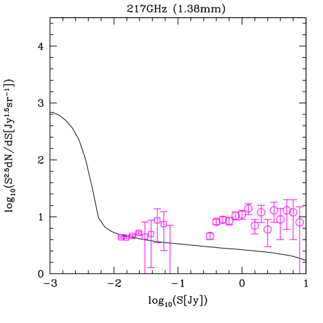
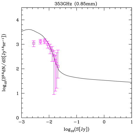
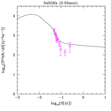
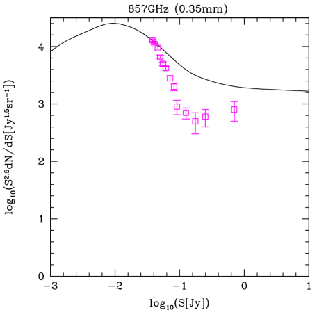
We first show the model predictions for the number counts of galaxies in the Planck HFI bands for which we later present clustering predictions. Fig. 3 shows the predicted differential galaxy counts and compares these with recent observational estimates. The top-right panel of Fig. 3 is an update of the comparison shown by Baugh et al. (2005) who considered the number counts. Baugh et al. showed that the MCGAL model reproduces the number counts and redshift distribution of m selected samples (see also Almeida et al. 2011). The recent measurements of the number counts at m, m and m using the Science Demonstration Phase data from the Herschel Space Telescope by Clements et al. (2011) and Oliver et al. (2011) suggest that the model predicts too many sources at bright fluxes (see predictions in Lacey et al. 2010). This is apparent from the comparison between model and observations in the other panels of Fig. 3.
The predictions for fluctuations in the CBL are sensitive to the flux-weighted abundance of galaxies. For example, the expression for the shot noise contribution to the angular power spectrum (Eq. 12) depends on the square of the flux. This is similar to the weighting of applied to the differential number counts in Fig. 3 (which is standard practice in the literature to expand the dynamic range of the counts). The dominant contribution to the shot noise is from fainter fluxes. The model predictions agree best with the observed counts at faint fluxes. The model overpredicts the counts at bright fluxes at m (GHz) and m (GHz) and underpredicts the counts at bright fluxes at m (GHz), which is due to the neglect of radio galaxies in the model.
3.2 The luminosity density of galaxies in the Planck bands
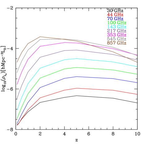
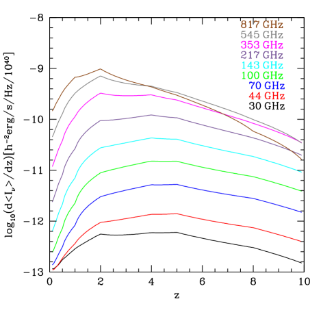
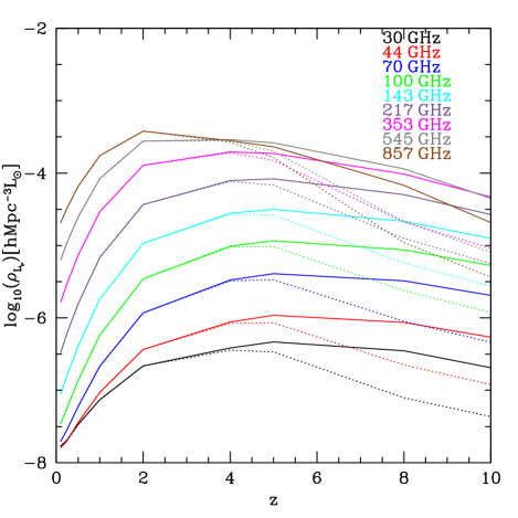
The luminosity density (; Eq. 10) in the Planck frequency bands is plotted in Fig. 4 as a function of redshift, computed using all of the galaxies in the MCGAL catalogue. At all nine Planck frequencies, the luminosity density increases from the present day up to – and then stays approximately constant or declines gently to . At a given redshift, the amplitude of the luminosity density increases with observer frame frequency because in the rest frame increases due to the shape of the SED (until the rest frame frequency moves past the peak in the dust emission spectrum). For a given observer frame frequency, the luminosity density is a combination of the SED sampled in the rest frame and the abundance of galaxies emitting at a given flux. The overall shape of the luminosity density as a function of redshift therefore tracks the star formation rate density in the universe, with a much gentler decline to high redshift, due to the increase in the rest frame (due to the negative -correction) offsetting the overall drop in star formation density.
The fraction of the overall luminosity density that is contributed by high redshift sources drops with increasing frequency, in agreement with previous interpretations of fluctuations in the CBL using empirical models (e.g. Hall et al. 2010).
The intensity fluctuation power spectrum depends on the mean intensity, which is an integral over the luminosity density as given by Eq. 6. From this equation, the contribution to the mean intensity per unit redshift interval is given by:
| (12) |
By plotting this quantity, we can see which redshifts contribute most to the mean intensity. Fig. 5 shows the contribution to the mean intensity with redshift in the Planck wavebands. A comparison between this plot and Fig. 4 shows that the mean intensity is dominated by lower redshifts than the luminosity density.
3.3 The clustering of SFGs in the Planck bands
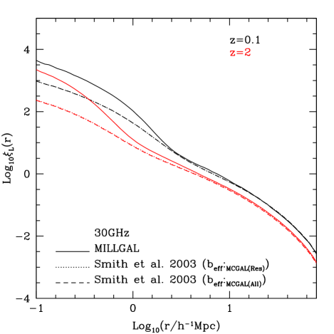
We now turn our attention to the computation of the flux correlation function. The use of the Millennium N-body simulation allows us to make accurate predictions for the clustering of galaxies on small and intermediate scales. This is illustrated in Fig. 6 which contrasts the direct estimate of the luminosity correlation function estimated from the MILLGAL catalogue with the analytic calculation based on the MCGAL catalogue. Recall that the pairwise galaxy counts are weighted by luminosity here. At small pair separations, Mpc, the N-body estimates are up to an order of magnitude larger than the analytic ones. Even though the analytic calculation takes into account the nonlinear form of the matter correlation function, the galaxy correlation function can be significantly different on these scales, since the analytic calculation ignores the 1-halo term (Benson et al. 2000). The differences between the two estimates persist to intermediate separations of a few megaparsecs, in the transition region from the one-halo to two-halo contributions to the correlation function.
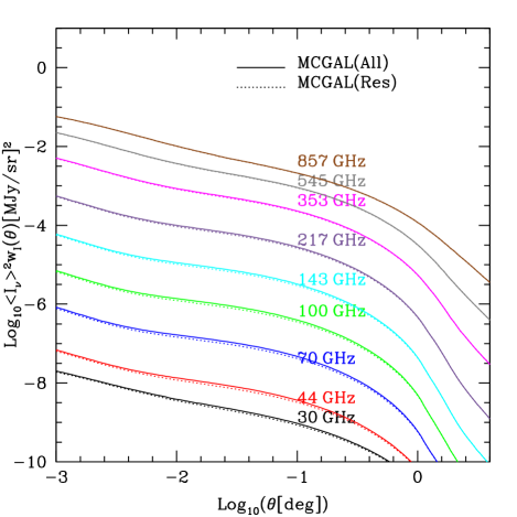
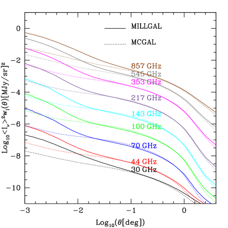
In Fig. 7 we take a step closer to the angular power spectrum of intensity fluctuations by plotting the angular flux correlation function multiplied by the square of the mean intensity fluctuations. We also compare the direct estimate of the clustering from the N-body simulation (solid lines) with the analytic one (dotted lines), for galaxies fainter than the Planck detection limits. The amplitude and shape of the two estimates of the correlation function are nearly the same at large angular separations. On small angular scales, e.g. degrees, the two estimates differ by up to an order of magnitude, due to the more accurate treatment of the 1-halo term and the transition between the 1- and 2-halo regimes in the N-body calculation (as seen in Fig. 6).

3.4 The angular power spectrum of fluctuations in the CBL from SFGs
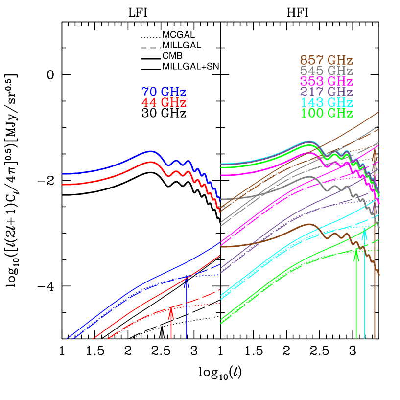
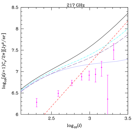
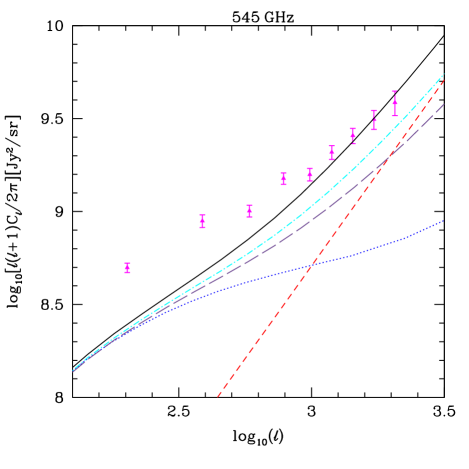
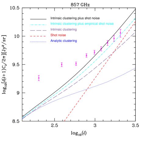
The main results of the paper are shown in Figs. 8 and 9. Fig. 8 shows the angular power spectrum of the intensity fluctuations of undetected galaxies in the Planck wavebands. Different components of the model predictions are shown in this plot. The long-dashed line shows the intrinsic clustering predicted using the N-body simulation, without any contribution from shot noise. This is to be contrasted with the dotted lines, which show the analytic clustering estimate. At small angular scales, , the N-body estimate exceeds the analytic one. Fig. 8 also lets us compare the amplitude of the fluctuations from extragalactic sources to the primordial CMB signal. In the LFI channels, the primordial signal dominates on all angular scales. At the HFI frequencies, the extragalactic and primordial signals become comparable above a particular value of . The angular power spectrum from undetected faint extragalactic sources exceeds the primordial power spectrum from at GHz, at GHz and for all angular scales at GHz.
Early measurements by Planck have been used to estimate the fluctuations in the CBL from unresolved extragalactic sources (The Planck Collaboration 2011b). As we have seen in Fig. 8, the primordial signal is orders of magnitude larger than the extragalactic signal at the lowest frequencies measured by Planck. Maps at these frequencies can be used to estimate the primordial signal expected in the higher frequency bands. These authors remove the Galactic foreground using observations of emission from neutral hydrogen to clean thermal dust emission. The estimated fluctuations in the cosmic infrared background due to the unresolved extragalactic sources are shown by the data points in Fig. 9. The error bars show the statistical and systematic errors (the area used covers 140 square degrees in six different fields). The systematic error, e.g. due to uncertainties in the beam, exceeds the statistical error at high in the higher frequency channels (see the Planck Collaboration 2011b for further details).
The theoretical predictions for the extragalactic intensity fluctuations in the CBL are considered more closely in Fig. 9. The shot noise computed from the MILLGAL model using Eq. 10 is shown by the short dashed line. The shot noise makes a fixed contribution to but has a scale dependence in Fig. 9 since here we plot . The contribution to from the intrinsic clustering of the unresolved galaxies, as estimated using the N-body based MILLGAL catalogue, is shown by the long dashed line. The corresponding analytical estimate is shown by the dotted line. At the smallest scales plotted, the N-body estimate exceeds the less accurate analytical one by a factor of three or more. The overall prediction for the intensity fluctuation power spectrum, combining the intrinsic clustering with the shot noise, is shown by the solid line. The shot noise makes an important contribution to the power spectrum at high . We have commented already that our model overpredicts the number counts of galaxies in the Herschel bands at bright fluxes. This will result in turn in an overprediction of the shot noise in these bands. To illustrate how this can affect our predictions, we also show a version of the power spectrum in which we replace the shot noise calculated using our model with that from the empirical number count model of Bethermin et al. (2011). This alternative prediction is shown by the dot-dashed line in Fig. 9. We note that these predictions are not meant to supersede those shown by the solid line, as now the number of sources is decoupled from the calculation of the intrinsic clustering.
Fig. 9 shows that the model predictions are generally within a factor of three or better of the observational estimate of the extragalactic background fluctuations. It is notable that in some of the HFI bands, the predicted shape of the power spectrum is similar to the observational estimate. The agreement between the model and observations is best at small angular scales in the two highest frequency channels. There is a mismatch in amplitude on larger scales (smaller ) in these higher frequency channels.
3.5 How can the model predictions be improved?
The goal of this paper is to present a new framework for predicting the contribution of star-forming galaxies to intensity fluctuations in the cosmic background light. We have used a previously published model to illustrate the technique. Unlike other studies in the literature, we have not varied any model parameters in order to improve the agreement of the model predictions with the signal inferred from observations.
Fig. 9 shows the model underpredicts the observed clustering on large angular scales in the two highest frequency HFI channels, whilst giving a reasonable match to the power spectrum on small scales. To improve the model predictions at GHz and GHz, we would need to increase the effective bias of the unresolved sources, whilst reducing their number slightly. This requires an increase in the typical effective host halo mass. Such a shift could be achieved by reducing the efficiency of star formation in galaxies hosted by low mass haloes.
On the other hand in the two lowest frequency channels shown in Fig. 9, GHz and GHz, the model overpredicts the clustering, so there needs to be a reduction in the effective host halo mass in these cases. We note that the model works best overall at GHz, the frequency at which the model was originally tuned to match the observed galaxy number counts and redshift distribution.
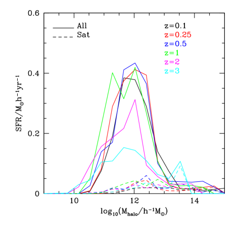
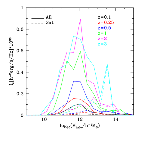
Fig. 10 gives some insight into which haloes dominate the clustering signal. The top panel of Fig. 10 shows the total star formation rate summing over galaxies in the same dark matter halo, plotted as a function of host halo mass. The y-axis is on a linear scale so that we can gain an impression of which haloes make the most important contribution to the overall star formation rate density (we would also need to take into account the halo mass function to connect this plot to the luminosity density). The distribution is dominated by central galaxies hosted by dark matter haloes with masses in the range -. In this paper we study correlations in intensity, so an important quantity to consider is the total luminosity per halo, summing over galaxies within the same dark matter halo, which is plotted as a function of host halo mass in the bottom panel of Fig. 10. The far-infrared luminosity depends on a galaxy’s star formation rate, along with its dust content and the level of extinction. The distribution of luminosity per halo has a similar form to that of the star formation rate, with a more pronounced tail to higher halo masses. This plot shows that the mass resolution of the Millennium N-body simulation is sufficient for modelling the intensity fluctuations of unresolved galaxies. To change the clustering predictions of the model, we need to move the location of the peak in the distribution plotted in Fig. 10, which means finding a way to put central galaxies of a given luminosity into different mass haloes, depending on the sense of the change required in the two-halo clustering term. The tail of satellite galaxies apparent in higher mass haloes influences the one-halo clustering term (i.e. pairs of galaxies within the same halo).
We have carried out a preliminary exploration of parameter space, changing one aspect of the model at a time, without trying to retain the previous successes of the model. We altered the strength of feedback from supernovae and experimented with deleting satellite galaxies assigned to subhaloes which can no longer be resolved in the Millennium Simulation. These changes produce a similar shift in the model predictions at each frequency and so do not produce the differential changes that we need to improve the match to the observations. A full, multi-dimensional parameter search to find a model with an improved match to the intensity fluctuations, which also reproduces the previous successful matches to observations, is beyond the scope of the current paper.
4 Conclusions
Fluctuations in the intensity of the microwave background radiation arise from a number of sources: ripples in the density of matter in the primordial Universe, emission from the interstellar medium in our galaxy, and extragalactic sources, such as star-forming galaxies (SFGs), radio galaxies or the hot plasma in galaxy clusters. Identifiable sources can be removed from intensity fluctuation maps. Sources below the confusion limits of the measurements cannot be explicitly excised. Their contribution can be removed statistically in analyses of the primordial signal or can be isolated to study the history of star formation in the Universe and its connection to structure formation in the dark matter.
Here we have introduced a hybrid model which combines a physical model of galaxy formation with a N-body simulation of the clustering of dark matter to predict the contribution of SFGs to the intensity fluctuations in the CBL. This is the first time that it has been possible to compute the abundance and clustering of SFGs together in a physical model. The model predicts the radio emission from star-forming galaxies and the emission from dust heated by stars, in a self consistent manner, with the dust grains in thermal equilibrium. The amount of heating depends on the star formation and chemical enrichment history of the galaxies, and on their dust mass and linear size; all of these properties are predicted by the model. Our calculation tells us how many galaxies above a stated flux limit should reside within dark matter haloes of a given mass. This information, in combination with an N-body simulation of the clustering of dark matter, allows a direct calculation of the clustering of SFGs. In previous calculations based on dark matter haloes, the halo occupation distribution was adjusted by hand, with no connection between the properties of the host halo and the spectral energy distribution of the galaxy.
We have illustrated this new framework using a published model of galaxy formation (Baugh et al. 2005). This model matches the observed galaxy number counts at 353 GHz (850 m), along with other observations of the galaxy population at low and high redshift. We have taken the predictions of this model without any adjustments. Hence, the example calculation we present is in effect parameter-free, since we make no further adjustment to the values of the parameters which specify the galaxy formation model. This is an important distinction of our work from halo occupation distribution modelling of the CBL fluctuations, in which case the model parameters are adjusted to improve the match to the measured clustering. In view of this, it is impressive that our predictions only disagree with the fluctuations in the CBL inferred from early Planck data by at worst a factor of three. It is also important to bear in mind that the observational estimate of the CBL fluctuations is heavily processed, and significant contributions from other sources have to be removed to isolate the extragalactic signal. Empirical calculations in the literature have a more limited scope than our model. Such calculations do contain parameters which are tuned to improve directly the agreement between the predicted and observed clustering. However, in general these models do not connect the emission from galaxies to their host dark matter haloes (for an exception see e.g. Shang et al. 2012).
Our model agrees best the inferred CBL fluctuations at high frequencies on small scales (high ), for which the shot noise from discrete sources and the clustering of galaxies within common dark matter haloes dominate, and where the isolation of the extragalactic signal is most secure. By using an N-body simulation, we are able to make accurate predictions for the one-halo as well as two halo contribution to the intensity fluctuations. These predictions are significantly different from simple analytical calculations on small angular scales. In general the model does less well on larger scales, around . This implies that the example model predicts the wrong effective bias or two-halo clustering term. At GHz, the predicted bias is too high by a factor of . At GHz, the effective bias predicted is too small by a similar factor (). As the intrinsic clustering dominates over the shot noise on these scales, this suggests that some redistribution of galaxies between dark matter haloes is required in the model. This is more difficult to realise than it may sound, as these adjustments would have to be made without changing the small-scale clustering by much. Of course, if the number of sources is also changed, then this will alter the shot noise, which mainly affects the amplitude of the small scale clustering. Another possible explanation for the discrepancy between the model predictions and the Planck results is that the emissivity of the dust assumed in the model may be incorrect. Baugh et al. modified the dust emissivity in bursts from the standard value of used in quiescent star formation to . This boosts the emission at longer wavelengths, and may in part be responsible for the excess counts at low frequencies.
As new observations of SFGs become available through, for example, the Herschel Space Observatory, new constraints will be placed on the galaxy formation model which underpins our method (Lacey et al. 2008; 2010). Along with improved treatments of key model ingredients, such as star formation (Lagos et al. 2010), this will allow us to devise new models which better match the new observations of SFGs. The clustering of intensity fluctuations in the CBL will offer an important additional observational constraint that such galaxy formation models will be able to exploit.
Acknowledgments
We acknowledge a helpful report from the referee. HSK acknowledges support from the Korean Government’s Overseas Scholarship. CSF acknowledges a Royal Society Wolfson Research Merit Award. SMC acknowledges the support of a Leverhulme Research Fellowship. This work was supported in part by a rolling grant from the Science and Technology Facilities Council.
References
- [1] Almeida C., Baugh C.M., Lacey C.G., 2011, MNRAS, 417, 2057
- [2] Amblard A., Cooray A., 2007, ApJ, 670, 903
- [3] Angulo R.E., Baugh C.M., Lacey C.G., 2008, MNRAS, 387, 921
- [4] Barger A. J., Cowie L. L., Sanders D. B., 1999, ApJ, 518, 5
- [5] Baugh C. M., Lacey C. G., Frenk C. S., Granato G. L., Silva L., Bressan A., Benson A. J., Cole S., 2005, MNRAS, 356, 1191
- [6] Baugh C. M., 2006, RPPh, 69, 3101
- [7] Benson A. J., Cole, S., Frenk C. S., Baugh C. M., Lacey C. G. 2000, MNRAS, 311, 739
- [8] Berlind A. A., Weinberg D. H., 2002, ApJ, 575, 587
- [9] Bertoldi F. et al., 2000, A&A, 360, 92
- [10] Bethermin M., Dole, H., Beelen, A., Aussel, H., 2010, A&A, 512, 78
- [11] Bethermin M., Dole, H., Lagache, G., Le Borgne D., Penin A., 2011, A&A, 529, 4
- [12] Borys C., Chapman S., Halpern M., Scott D., 2003, MNRAS, 344, 385
- [13] Bower R.G., Benson A.J., Malbon R., Helly J.C., Frenk C.S., Baugh C.M., Cole S., Lacey C.G., 2006, MNRAS, 370, 645
- [14] Bressan A., Silva L., Granato G. L., 2002, A& A, 392, 377
- [15] Chapman S. C., Scott D., Borys C., Fahlman G. G., 2002, MNRAS, 330, 92
- [16] Clements D.L., et al. 2010, A&A, 518, L8
- [17] Cole S., Lacey C. G., Baugh C. M., Frenk C. S., 2000, MNRAS, 319, 168
- [18] Condon J. J., ARA&A, 30, 575.
- [19] Coppin K., et al. 2006, MNRAS, 372, 1621
- [20] Cowie L. L., Barger A. J., Kneib J.-P., 2002, AJ, 123, 2197
- [21] Dole H. et al., A&A, 372, 364
- [22] Dole H. et al., 2004, ApJS, 154, 93
- [23] Dunkley J., et al., 2011, ApJ, 739, 52
- [24] Elbaz D., Cesarsky C. J., Chanial P., Aussel H., Franceschini A., Fadda D., Chary R. R., 2002, A&A, 384, 848
- [25] Eke V., Cole S., Frenk C.S., Navarro J.F., 1996, MNRAS, 281, 703
- [26] Fernandez-Conde N., Lagache G., Puget J.-L., Dole H., 2008, A&A, 481, 885
- [27] Gao L., Springel V., White S.D.M., 2005, MNRAS, 363, L66
- [28] Genzel R., Cesarsky C. J., 2000, ARA&A, 38, 761
- [29] Gonzalez-Nuevo J., Toffolatti L., 2005, ApJ, 621, 1
- [30] Granato G. L., Lacey C. G., Silva L., Bressan A., Baugh C. M., Cole S., Frenk C. S., 2000, ApJ, 542, 710
- [31] Granato G. L., De Zotti G., Silva L., Bressan A., Danese L., 2004, ApJ, 600, 580
- [32] Grossan B, Smoot G.F., 2007, A&A, 474, 731
- [33] Haiman Z., Knox L., 2000, ApJ, 530, 124
- [34] Hall N.R., et al. 2010, ApJ, 718, 632.
- [35] Holland W. S., Greaves J. S., Zuckerman B., Webb R. A., McCarthy C., Coulson I. M., Walther D. M., Dent W. R. F. et al., 1998, Nature, 392, 788
- [36] Kennicutt R. C. Jr., 1983, ApJ, 272, 54
- [37] Kennicutt R. C. Jr., 1998, ARA&A, 36, 189
- [38] Kim H.-S, Baugh C. M., Cole S., Frenk C. S., Benson A. J., 2009, MNRAS, 400, 1527
- [39] Knox L., Cooray A., Eisenstein, D., Haiman Z., 2001, ApJ, 550, 7
- [40] Komatsu E., et al. 2011, ApJS, 192, 18.
- [41] Kroupa P., Aarseth S., Hurley J., 2001, MNRAS, 321, 699
- [42] Lacey C., Cole S., 1993, MNRAS, 262, 627
- [43] Lacey C. G., Baugh C. M., Frenk C. S., Silva L., Granato G. L., Bressan A., 2008, MNRAS, 385, 1155
- [44] Lacey C. G., Baugh C. M., Frenk C. S., Benson A. J., Orsi A., Silva L., Granato G. L., Bressan A., 2010, MNRAS, 405, 2
- [45] Lacey C.G., Baugh C.M., Frenk C.S., Benson A.J., 2011, MNRAS, 412, 1828
- [46] Lagache G., Dole H., Puget J.-L., 2003, MNRAS, 338, 555
- [47] Lagache G., Bavouzet N., Fernandez-Conde N., Ponthieu N., Rodet T., Dole, H., Miville-Deschenes M.-A., Puget J.-L., 2007, ApJ, 665, L89.
- [48] Le Delliou M., Lacey C., Baugh C. M., Morris S. L., 2006, MNRAS, 365, 712
- [49] Negrello M., Perrotta F., Gonzalez-Nuevo J., Silva L., de Zotti G., Granato G. L., Baccigalupi C., Danese L., 2007, MNRAS, 377, 157
- [50] Neistein E., Maccio A. V., Dekel A., 2010, MNRAS, 403, 984
- [51] Oliver S.J., et al., 2011, A&A, 518, L21
- [52] Orsi A., Lacey C. G., Baugh C. M., Infante L., 2008, MNRAS, 391, 1589
- [53] Papovich C. et al., 2004, ApJS, 154, 70
- [54] Parkinson H., Cole S., Helly J., 2008, MNRAS, 383, 557
- [55] Peacock J. A., Smith R. E., 2000, MNRAS, 318, 1144
- [56] Planck Collaboration, 2011a, 2011, A&A, 536, A1
- [57] Planck Collaboration, 2011b, 2011, A&A, 536, A18
- [58] Planck Collaboration, 2011c, 2011, A&A, 536, A5
- [59] Planck Collaboration, 2011d, 2011, A&A, 536, A6
- [60] Planck Collaboration, 2011e, 2011, A&A,536, A13
- [61] Penin A., et al. 2012a, A&A in press, arXiv1105.1463
- [62] Penin A., Dore O., Lagache G., Bethermin M., 2012b, A&A, 537, A137
- [63] Righi M., Hernandez-Monteagudo C., Sunyaev R. A., 2008, A&A, 478, 685
- [64] Scott S. E., Fox M. J., Dunlop J. S., Serjeant S., Peacock J. A., Ivison R. J., Oliver S., Mann R. G. et al., 2002, MNRAS, 331,817
- [65] Sehgal N., et al., 2010, ApJ, 709, 920
- [66] Shang C., Haiman Z., Knox L., Oh S. P., 2012, MNRAS, 421, 2832
- [67] Sheth R. K., Mo H. J., Tormen G., 2001, MNRAS, 323, 1
- [68] Silva L., Granato G. L., Bressan A., Danese L, 1998, ApJ, 509, 103
- [69] Smail I., Ivison R. J., Blain A. W., Kneib J.-P., 2002, MNRAS, 331, 495
- [70] Smith R. E., Peacock J. A., Jenkins A., White S. D. M., Frenk C. S., Pearce F. R., Thomas P. A., Efstathiou G., Couchman H. M. P., 2003, MNRAS, 341, 1311
- [71] Song Y. -S., Cooray A., Knox L., Zaldarriaga M., 2003, ApJ, 590, 664
- [72] Springel V., et al. 2005, Nature, 435, 629
- [73] Sunyaev R. A., Zel’dovich Ia. B., 1980, ARA&A, 18, 537
- [74] Tegmark M., Efstathiou G., 1996, MNRAS, 281, 1297
- [75] Vega O., Clemens M. S., Bressan A., Granato G. L., Silva L., Panuzzo P., 2008, A&A, 484, 631
- [76] Vielva P., Mart nez-Gonz lez E., Gallegos J. E., Toffolatti L., Sanz J. L., 2003, MNRAS, 344, 89
- [77] Viero M. P., et al., 2009, ApJ, 707, 1766
- [78] Xia J., Negrello M., Lapi A., de Zotti G, Danese L., Viel M., 2012, MNRAS, in press.
Appendix
The halo mass resolution of the MCGAL catalogue is essentially arbitrary, as the full memory of the computer can be devoted to a single dark matter halo merger history. Furthermore, the mass resolution can be adjusted with redshift, to ensure that a representative sample of halo masses is modelled at each epoch. The mass resolution of the MILLGAL sample is set by the Millennium N-body simulation and is fixed at all redshifts. In this Appendix we compare results from the two calculations to demonstrate the impact that the finite resolution of the MILLGAL sample has on our model predictions. We conclude that the predictions for the intensity fluctuations are insensitive to the resolution of the Millennium Simulation.
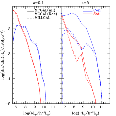
We first consider the luminosity functions predicted in the two catalogues in Fig. 11. At low redshift, the MILLGAL and MCGAL catalogues are in very good agreement with one another, both for central and satellite galaxies (i.e. at in the left panel of Fig. 11). The luminosity function of the two catalogues differ at high redshift because the MILLGAL does not include galaxies hosted by haloes below the mass resolution of the Millennium simulation. However, the MILLGAL catalogue reproduces well the luminosity function of the MCGAL catalogue at higher luminosities, at which the galaxies tend to be hosted by more massive dark matter haloes which are resolved in Millennium simulation (see the right panel in Fig. 11).
In Fig. 12, the luminosity density of galaxies hosted by dark matter haloes resolved by the Millennium simulation is lower than that of all the galaxies in the MCGAL catalogue for . Galaxies in low mass dark matter haloes contribute significantly to the luminosity density at high .
In Fig. 13, we plot the integrated luminosity weighted bias. The result shows that there is little impact on this measure of the intensity fluctuations on applying the resolution limit of the N-body simulation to the MCGAL catalogue.
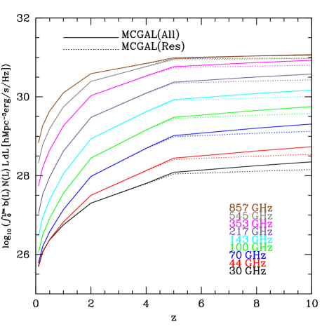
The similarity between the results shown in Fig. 13 for different halo mass resolution limits and the fact that the mean intensity is dominated by low redshifts imply that our predictions for the power spectrum of intensity fluctuations should be insensitive to the resolution limit of the MCGAL catalogue. This is confirmed in Fig. 14 in which we plot the analytic estimate of the product of the square of the mean intensity and the angular correlation function of intensity using the MCGAL catalogue. The predictions for the full MCGAL catalogue are indistinguishable from those restricted to galaxies which could be resolved in the Millennium simulation.