Exact Coleman-De Luccia Instantons

Abstract

We present exact Coleman-De Luccia (CDL) instantons, which describe vacuum decay from Anti de Sitter (AdS) space, de Sitter (dS) space and Minkowski space to AdS space. We systematically obtain these exact solutions by considering deformation of Hawking-Moss (HM) instantons. We analytically calculate the action of instantons and discuss a subtlety in calculation of decay rates.

I Introduction

The development of string theory has revealed a vacuum structure of the universe, so-called “the string theory landscape” where many metastable vacuum states exist. Then, the study of CDL instantons Coleman:1980aw describing the decay of such metastable states has attracted much interest recently. The vacuum decay in a fixed background has been well understood thanks to the seminal papers by Coleman and his collaborators Coleman:1977py ; Callan:1977pt . However, tunneling in the presence of gravity is still controversial. For example, the existence of negative modes may be gauge dependent for CDL instanton solutions Tanaka:1992zw ; Tanaka:1998mp ; Tanaka:1999pj ; Khvedelidze:2000cp . Hence, interpretation of the CDL instantons is not so clear . Moreover, there exist some claims on the string theory landscape that contradict each other. It is claimed that the eternal inflation may populate the string theory landscape Brown:2011ry . On the other hand, it is insisted that one of the effects of gravitational backreaction might be missing in the thin-wall approximation for the CDL instantons Copsey:2011zj . Then the decay rate is enhanced if we take into account the effect. It implies that most of vacua rapidly decay and the string theory landscape would not be relevant to cosmology. Furthermore, there is a dispute on the interpretation of the decay rate of the metastable vacuum into an AdS vacuum Dvali:2011wk ; Garriga:2011we . Thus, it is worth pursuing the study of the vacuum decay with gravity.

It would be beneficial if we had an analytic treatment of the CDL instanton solutions describing the vacuum decay with gravity. So far, the only available tool has been the thin-wall approximation. However, since the string theory landscape has a variety of vacua, there is a limitation of the thin-wall approximation. Of course, one can resort to the numerical analysis. However, it is difficult to grasp the physics behind numerical calculations. Therefore, we need analytical tools beyond the thin-wall approximation. In fixed background cases, it is not so difficult to construct exactly solvable models Hamazaki:1995dy ; Koyama:1999ai ; Pastras:2011zr ; Dutta:2011ej ; Dutta:2011rc . Recently, an attempt to construct analytic CDL solutions has been performed Dong:2011gx . The method is well known in the literature of braneworld  DeWolfe:1999cp ; Gremm:1999pj ; Csaki:2000fc ; Kobayashi:2001jd . However, they did not get analytic forms of potential functions Dong:2011gx . In this paper, we present exact CDL instantons for the first time by focusing on the HM instantons Hawking:1981fz . The HM instantons, which are nothing but Euclidean dS solutions, play an important role when the CDL instantons disappear. When the curvature scale of the potential barrier is large compared to the scale determined by the potential energy, CDL instantons exist. As the curvature scale becomes small, however, the CDL instantons approach and eventually merge into the HM instantons. Hence, it is expected that we can construct the CDL instantons by making deformation of the Euclidean dS solutions. Indeed, we find many exact CDL instantons using this strategy. In particular, we find potentials for which we can construct exact CDL instantons. Using our exactly solvable models, we can calculate decay rates analytically.

So far, vacuum decays from dS to dS and from dS to Minkowski have been well discussed in conjunction with cosmology. However, recent string theory landscape picture tells us the importance of AdS vacua. Hence, our primary interest in this paper is the vacuum decay rate to the AdS vacuum. We note that Banks argued that the decay to an AdS crunch is an actual fate of the decay process Banks:2002nm . Using our exactly solvable models, we investigate various decay processes. In addition to these practical calculations, we will discuss a subtle point related to the interpretation of CDL instantons.

The organization of this paper is as follows. In section II, we give basic equations and a strategy to find exact solutions. In section III, we present exact solutions which describe vacuum decay from AdS space, dS space and Minkowski space to AdS space. In section IV, we calculate the action of instantons. In section V, we evaluate decay rates for various decay processes. We find there exists a subtlety in evaluating decay rates simply by following a CDL prescription. Section VI is devoted to conclusion.

II Coleman-De Luccia Set up

Suppose that there are two perturbatively stable vacua and one of them is a metastable false vacuum. The false vacuum will decay into a true vacuum. The decay process can be described by an instanton in a semi-classical approximation. In the absence of gravity, a method for the instanton is well established. On the other hand, in the presence of gravity, it is believed that CDL instantons play an important role. In this section, we set up basic equations for obtaining the CDL instantons and describe a strategy to get exact solutions.

We begin with $d$-dimensional Euclidean action for the gravitational field $g_{\mu\nu}$ and the scalar field $\phi$:

$$S_{E}=-\frac{1}{2\kappa^{2}}\int_{M}d^{d}x\sqrt{g}~{}R-\frac{1}{\kappa^{2}}\int_{\partial M}d^{d-1}x\sqrt{h}~{}K+\int_{M}d^{d}x\sqrt{g}\left[~{}\frac{1}{2}g^{\mu\nu}\partial_{\mu}\phi\partial_{\nu}\phi+V(\phi)~{}\right]\,,$$ (1)

where $\kappa^{2}=8\pi G$, $R$ is the Ricci scalar for the metric $g_{\mu\nu}$, $K$ is the trace part of the extrinsic curvature and $h$ is the determinant of an induced metric on the boundary. The second term is the Gibbons-Hawking (GH) term which is necessary to make the variational principle consistent Gibbons:1976ue . This action is well defined for spatially compact geometries but diverges for non-compact ones. Hence, the physical action is required to take the form Hawking:1995fd

$$I=S_{E}\left[~{}g_{\mu\nu},~{}\phi~{}\right]-S_{b}\left[~{}g_{b\mu\nu},~{}\phi_{b}~{}\right]\ ,$$ (2)

so that the physical action of the reference background becomes zero. Here, suffix $b$ represents the background.

According to this prescription, the appropriate action for asymptotically flat space is expressed by

$$I=-\frac{1}{2\kappa^{2}}\int_{M}d^{d}x\sqrt{g}~{}R-\frac{1}{\kappa^{2}}\int_{\partial M}d^{d-1}x\sqrt{h}~{}[K-K_{0}]+\int_{M}d^{d}x\sqrt{g}\left[~{}\frac{1}{2}g^{\mu\nu}\partial_{\mu}\phi\partial_{\nu}\phi+V(\phi)~{}\right]\ ,$$ (3)

where $K_{0}$ is the trace of the extrinsic curvature of the boundary embedded in flat space Gibbons:1976ue ; Hawking:1995fd . Apparently, this action vanishes for the flat space. For other backgrounds, we need to go back to the more general form in Eq. (2). In the process of a vacuum decay, the choice of $S_{b}$ is a subtle issue as we will see later in Section V.

It is believed that the vacuum decay is described by $O(d)$ symmetric instantons. Then, we take the metric with $O(d)$ symmetry of the form

$$ds^{2}={\cal N}(\xi)^{2}d\xi^{2}+a(\xi)^{2}d\Omega^{2}_{d-1}\ .$$ (4)

Here, ${\cal N(\xi)}$ and $a(\xi)$ are the lapse function and the scale factor of the coordinate $\xi$, respectively. $d\Omega^{2}_{d-1}$ is the line element of a unit $(d-1)$-dimensional sphere. The action with this metric is given by

$$S_{E}=-\frac{(d-1)(d-2)}{2\kappa^{2}}v_{S^{d-1}}\int d\xi\left[~{}\frac{1}{\cal N}a^{d-3}a^{\prime 2}+{\cal N}a^{d-3}~{}\right]+v_{S^{d-1}}\int d\xi~{}a^{d-1}\left[~{}\frac{1}{2{\cal N}}\phi^{\prime 2}+{\cal N}V~{}\right]\ ,$$ (5)

where a prime denotes derivative with respect to $\xi$ and $v_{S^{d-1}}$ is a volume of the unit $(d-1)$-dimensional sphere. Note that the internal scalar curvature of a unit sphere is $R^{(d-1)}=(d-1)(d-2)$. The GH term canceled the surface term of the Einstein-Hilbert action.

Varying the action with respect to ${\cal N}$ and ${\phi}$ gives the following basic equations. We set ${\cal N}=1$ after the variation. The Hamiltonian constraint equation is given by

$$\left(\frac{a^{\prime}}{a}\right)^{2}=\frac{1}{a^{2}}+\frac{2\kappa^{2}}{(d-1)(d-2)}\left(\frac{1}{2}\phi^{\prime 2}-V\right)\ .$$ (6)

The scalar field equation becomes

$$\phi^{\prime\prime}+(d-1)\frac{a^{\prime}}{a}\phi^{\prime}-\frac{dV}{d\phi}=0\ .$$ (7)

The equation obtained by taking the variation with respect to $a(\xi)$ is redundant. By taking the derivative with respect to $\xi$ of Eq. (6) and plugging the Eq. (7) into it, we find the derivative of the scalar field is written only by the scale factor. Furthermore, putting the result back into Eq. (6), we get the potential for the scalar field expressed only by the scale factor as well. Then the basic equations become

$$\frac{\kappa^{2}}{d-2}\phi^{\prime 2} = \left(\frac{a^{\prime}}{a}\right)^{2}-\frac{1}{a^{2}}-\frac{a^{\prime\prime}}{a}\ ,$$ (8)

$$\frac{2\kappa^{2}}{(d-2)^{2}}V(\phi) = \frac{1}{a^{2}}-\left(\frac{a^{\prime}}{a}\right)^{2}-\frac{1}{d-2}\frac{a^{\prime\prime}}{a}\ .$$ (9)

Thus, if we put a desired function for $a(\xi)$ in these equations, both of the derivative of the scalar field and the potential of the scalar field are given as a function of $\xi$ from Eqs. (8) and (9). Combining those results, we then get the form of $V(\phi)$. The potential we look for is to have metastable and stable vacuum points and the metastable vacuum will eventually decay into the true vacuum.

In order to find CDL instanton solutions, it is convenient to move to the conformal coordinate defined by $d\xi=a(z)dz$, which corresponds to the choice ${\cal N}=a$. Then, Eqs. (8) and (9) become

$$\frac{\kappa^{2}}{d-2}\left(\frac{d\phi}{dz}\right)^{2} = \frac{2}{a^{2}}\left(\frac{da}{dz}\right)^{2}-\frac{1}{a}\frac{d^{2}a}{dz^{2}}-1\ ,$$ (10)

$$\frac{2\kappa^{2}}{(d-2)^{2}}V(\phi) = \frac{1}{a^{2}}\left[~{}1-\frac{d-3}{d-2}\frac{1}{a^{2}}\left(\frac{da}{dz}\right)^{2}-\frac{1}{d-2}\frac{1}{a}\frac{d^{2}a}{dz^{2}}~{}\right]\ .$$ (11)

In the next section, we will present a deformation method for obtaining exact CDL instantons using this strategy. It is not difficult to perform our analysis in arbitrary dimensions, however, we will concentrate on exact solutions in four dimensions $(d=4)$ for simplicity.

III Exactly Solvable Models

In this section, we present exactly solvable models of the vacuum decay with gravity. As we explained in the previous section, we give some scale factors $a(z)$ first. As a key to find exact solutions, we focus on the HM instantons which are Euclidean dS solutions Hawking:1981fz . If the potential satisfies the condition $3|V^{\prime\prime}|>4\kappa^{2}V$ at the maximal point of the potential barrier, both of the CDL and HM instantons exist Jensen:1983ac . In this case, the CDL instantons describe the decay of a false vacuum. However, if the potential does not satisfy this condition, the CDL instantons do not exist anymore . Instead, the HM instantons describe the decay of the false vacuum. This implies that the CDL instantons approach to the HM instantons as $3|V^{\prime\prime}|$ approaches $4\kappa^{2}V$, and eventually degenerate into the HM instantons. There the scale factor is given by $a(z)=\ell_{\rm dS}/\cosh z$, where $\ell_{\rm dS}$ is the curvature radius in the Euclidean dS spaces. Since the HM instanton is a limit of the CDL instanton, we can make use of deformation of HM instantons for obtaining the CDL instantons. Namely, we can put the ansatz for the scale factor

$$a(z)=\ell~{}\frac{f\left(\tanh z\right)}{\cosh z}\ ,$$ (12)

where we refer a function of $\tanh z$, $f$, as the deformation function from the HM instantons. Here, $\ell$ is a length scale in the system. This function guarantees a compact asymptotic structure at $z\rightarrow\infty$. Substituting this into Eq. (10), we obtain

$$\frac{\kappa^{2}}{4}\left(\frac{d\phi}{d\lambda}\right)^{2}=\left(\frac{1}{f}\frac{df}{d\lambda}\right)^{2}-\frac{1}{2f}\frac{d^{2}f}{d\lambda^{2}}\,,$$ (13)

where we defined a variable $\lambda=\tanh z$. Using the function $f$, we can write the potential as

$$\frac{\kappa^{2}\ell^{2}}{2}V=\frac{1}{f^{2}}\left[~{}\frac{3}{2}-\frac{1}{2}\left(1-\lambda^{2}\right)\frac{1}{f}\frac{d^{2}f}{d\lambda^{2}}+3\lambda~{}\frac{1}{f}\frac{df}{d\lambda}-\frac{1}{2}\left(1-\lambda^{2}\right)\left(\frac{1}{f}\frac{df}{d\lambda}\right)^{2}~{}\right]\ .$$ (14)

Now, we can discuss various exact solutions using the above formulas.

III.1 From Runaway State to AdS

III.1.1 Type $f(\lambda)=\exp\left(\alpha\lambda\right)$

Looking at Eq. (13), we find a kink type solution proportional to $\lambda$. Indeed, we can choose the deformation function as

$$f(\lambda)=\exp\left(\alpha\lambda\right)\ ,$$ (15)

which leads to the scale factor

$$a(z)=\ell~{}\frac{e^{\alpha\tanh z}}{\cosh z}\ ,$$ (16)

where $\alpha$ is a constant parameter. This scale factor has a profile deformed from Euclidean dS spaces, $\alpha=0$, (see Fig. 2 ). Interestingly, it turns out that this simple deformation changes the constant potential corresponding to the Euclidean dS space into a runaway potential. Plugging Eq. (15) into Eq. (13) and integrating it, we get the scalar field

$$\frac{\kappa}{2}\phi=\frac{\alpha}{\sqrt{2}}\lambda=\frac{\alpha}{\sqrt{2}}\tanh z\ ,$$ (17)

where we took a plus sign of $\phi$ and put the constant of integration zero. A minus sign corresponds to a parity flip $z\rightarrow-z$. We have plotted the profile of the scalar field in Fig. 2. Since $|\tanh z|<1$, the range of the scalar field is restricted to $-\frac{\sqrt{2}\alpha}{\kappa}<\phi<\frac{\sqrt{2}\alpha}{\kappa}$. The CDL instanton is restricted to this range in this way.

Figure 1: The scale factor as a function of $z$ with $\ell=1$. A solid line corresponds to $\alpha=0.1$. A dashed line corresponds to the dS solution $\alpha=0$.

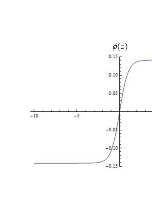
Figure 2: The scalar field as a function of $z$ in the case of $\alpha=0.1$. $\kappa=1$.

Putting the scale factor Eq. (16) into Eq. (14), we can calculate the potential $V$ as a function of $z$

$$\kappa^{2}\ell^{2}~{}V=\frac{1}{2\cosh^{2}z}e^{-2\alpha\tanh z}\left(~{}3-4\alpha^{2}+3\cosh 2z+6\alpha\sinh 2z~{}\right)\ .$$ (18)

As we can solve $\tanh z$ as a function of $\phi$ from Eq. (17), if we substitute it into Eq. (18), the potential $V$ is obtained as a function of $\phi$

$$\kappa^{2}\ell^{2}~{}V(\phi)=e^{-\sqrt{2}\kappa\phi}\left(~{}3-2\alpha^{2}+3\sqrt{2}\kappa\phi+\kappa^{2}\phi^{2}~{}\right)\ .$$ (19)

The potential has a runaway shape as in Fig. 3, namely, there is no true minimum in the false vacuum side. In Fig. 3, a green line shows the range of the CDL instanton. This instanton solution can be interpreted as a decay process from the runaway state to an AdS vacuum. After the tunneling, the scalar field will roll down the potential and follows Lorentzian equations.

Note that we can deform the potential keeping the shape of the green line fixed. This means that we can also interpret that the instanton mediates the tunneling between two dS vacua in the case of Fig. 3.

Figure 3: The potential as a function of $\phi$ in the case of $\alpha=0.1$. $\kappa=\ell=1$. The true vacuum is an AdS vacuum. The metastable false vacuum is a Minkowski vacuum at the infinity of $\phi$. The instanton describing the vacuum decay is shown in a green line.

III.1.2 Type $f(\lambda)=1+\beta\lambda$

Another simple choice is to take $d^{2}f/d\lambda^{2}=0$ in Eq. (13). Then the deformation function becomes

$$f(\lambda)=1+\beta\lambda\ ,$$ (20)

where $\beta$ is a constant parameter. The scale factor is then given by

$$a(z)=\ell~{}\frac{1+\beta\tanh z}{\cosh z}\ .$$ (21)

Here, we have to impose the condition $0<\beta<1$ to get a positive scale factor $a$. Changing the sign of $\beta$ corresponds to a parity flip $z\rightarrow-z$. Putting Eq. (20) into Eq. (13) and integrating it over, we obtain the scalar field of this form

$$\frac{\kappa}{2}\phi=\log\left(1+\beta\lambda\right)=\log\left(1+\beta\tanh z\right)\ .$$ (22)

Since $|\tanh z|<1$, the range of the scalar field is restricted to $1-\beta<e^{\frac{\kappa}{2}\phi}<1+\beta$. Using Eq. (14), we can also calculate the potential $V$ as a function of $z$

$$\kappa^{2}\ell^{2}~{}V=\frac{3}{\left(1+\beta\tanh z\right)^{2}}-\frac{\beta^{2}\left(1-\tanh^{2}z\right)}{\left(1+\beta\tanh z\right)^{4}}+\frac{6\beta\tanh z}{\left(1+\beta\tanh z\right)^{3}}\ .$$ (23)

As we can solve $\tanh z$ as a function of $\phi$ from Eq. (22), if we substitute it into Eq. (23), we can deduce the potential $V$ as a function of $\phi$

$$\kappa^{2}\ell^{2}~{}V(\phi)=10e^{-\kappa\phi}-8e^{-\frac{3}{2}\kappa\phi}+\left(1-\beta^{2}\right)e^{-2\kappa\phi}\ .$$ (24)

With the parameters $\ell=3.8\ ,\ell\beta=0.8$, we have the similar potential as the previous case as in Fig. 5. The green line shows the range of the instanton. We note that this type of potential often appears in flux compactification models. In the context of the flux compactification, the scalar field $\phi$ plays a roll of a radion field and runs away towards the Minkowski vacuum $\phi\rightarrow\infty$, which is interpreted as a de-compactification in flux compactification models  BlancoPillado:2009di ; BlancoPillado:2009mi .

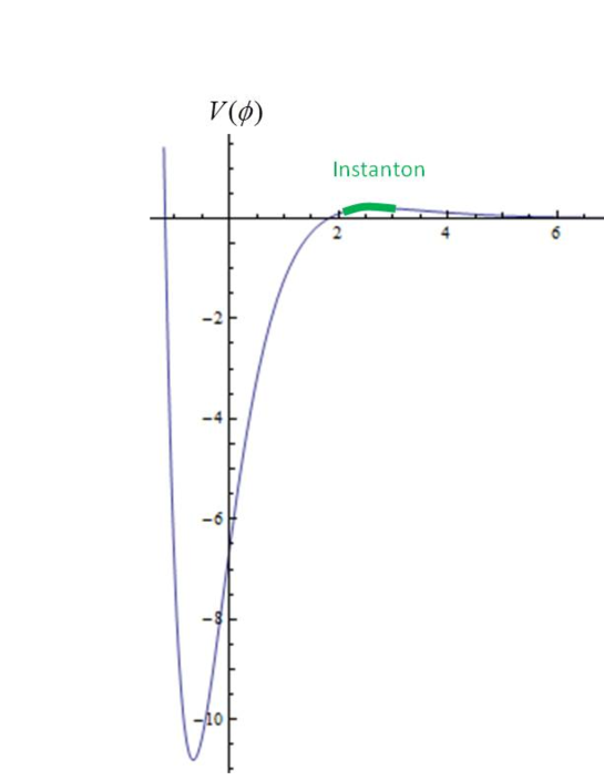
Figure 4: The potential, $V$ versus $\phi$ in the case of $\ell=3.8,~{}\ell\beta=0.8$ in type $f(\lambda)=1+\beta\lambda$ model. $\kappa=1$. A green line shows by the CDL instanton.

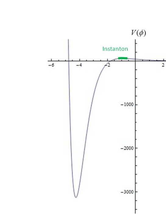
Figure 5: The potential, $V$ versus $\phi$ in the case of $\alpha=3,~{}\beta=1,~{}\ell=2,~{}\ell\gamma=1$ in type $f(\lambda)=\left(1+\gamma\lambda\right)/\left(\alpha+\beta\lambda\right)^{2}$ model. $\kappa=1$. The green line shows the CDL instanton.

III.1.3 Type $f(\lambda)=\left(1+\gamma\lambda\right)/\left(\alpha+\beta\lambda\right)^{2}$

As an extension of the form Eq. (20), we find

$$f(\lambda)=\frac{1+\gamma\lambda}{\left(\alpha+\beta\lambda\right)^{2}}$$ (25)

is also solvable. Here, $\alpha,\beta$ and $\gamma$ are constant parameters. The scale factor reads

$$a(z)=\frac{1+\gamma\tanh z}{\left(~{}\alpha+\beta\tanh z~{}\right)^{2}}\cdot\frac{\ell}{\cosh z}\ .$$ (26)

Here, we have to impose the condition $0<\gamma<1$ and $|\beta|<\alpha$ to get a positive scale factor $a$. Eq. (13) gives a simple expression

$$\frac{\kappa}{2}\frac{d\phi}{d\lambda}=\frac{\alpha\gamma-\beta}{\left(\alpha+\beta\lambda\right)\left(1+\gamma\lambda\right)}\ .$$ (27)

Note that we took one of sign of $\pm$ of this result simply because the other sign just changes $\phi$ to $-\phi$. We can integrate it such as

$$\frac{\kappa}{2}\phi=\log\left(\frac{1+\gamma\tanh z}{\alpha+\beta\tanh z}\right)\ .$$ (28)

Since $|\tanh z|<1$, the region of the scalar field is restricted to $\frac{2}{\kappa}\log\big{|}\frac{1-\gamma}{\alpha-\beta}\big{|}<\phi<\frac{2}{\kappa}\log\big{|}\frac{1+\gamma}{\alpha+\beta}\big{|}$ (see Fig. 5 ). Thus the potential is obtained in the same way as previous cases

$$\kappa^{2}\ell^{2}V(\phi)=10\left(\alpha^{2}-\beta^{2}\right)e^{-\kappa\phi}-8\left(\alpha-\beta\gamma\right)e^{-\frac{3}{2}\kappa\phi}+\left(1-\gamma^{2}\right)e^{-2\kappa\phi}\ ,$$ (29)

where we used the inversion $\tanh z=\frac{1-\alpha e^{\frac{\kappa}{2}\phi}}{\beta e^{\frac{\kappa}{2}\phi}-\gamma}$ in Eq. (28). We get a runaway type potential with an AdS minimum again.

We see that those instantons do not tunnel from a local minimum to a local minimum of the potential. This is the effects of gravity. Thus it is difficult to read off the false and true vacuum of the potential without knowing the whole shape of it.

III.2 From vacuum to vacuum

Let us obtain the CDL instantons for the potentials having two vacua. For this purpose, it is useful to rewrite the right hand side of Eq. (13) as

$$\frac{\kappa^{2}}{4}\left(\frac{d\phi}{d\lambda}\right)^{2}=\frac{f}{2}\frac{d^{2}}{d\lambda^{2}}\left(\frac{1}{f}\right)\ .$$ (30)

We consider $d^{2}/d\lambda^{2}(1/f)=~{}$const. in the above equation as a simple choice. This gives

$$f(\lambda)=\frac{1}{1+\beta\lambda+\gamma\lambda^{2}}\ ,$$ (31)

where $\beta,\gamma$ are constant parameters. That is, the scale factor is expressed by

$$a(z)=\frac{1}{1+\beta\tanh z+\gamma\tanh^{2}z}\cdot\frac{\ell}{\cosh z}\ .$$ (32)

Here, we have to impose conditions on parameters so that the scale factor is positive. Substituting this expression into Eq. (13), we find the derivative of the scalar field of this form

$$\kappa^{2}\phi^{\prime 2}=\frac{4\gamma}{1+\beta\tanh z+\gamma\tanh^{2}z}\cdot\frac{1}{\cosh^{4}z}\ .$$ (33)

Thus, we will have three kinds of potentials according to the discriminant of the quadratic polynomial of $\tanh z$ in the denominator.

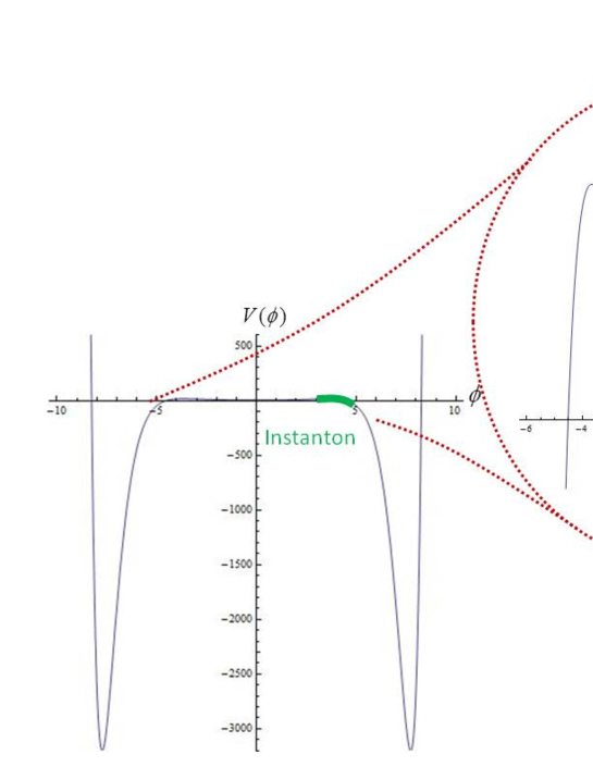
Figure 6: The potential, $V$ versus $\phi$ for $\ell=0.25,~{}\beta=4.1\ell,~{}\gamma=\ell$. $\kappa=1$. The region around a metastable dS vacuum is enlarged in a red circle.

III.2.1 From dS to AdS

First, we consider the case $\beta^{2}-4\gamma>0$. We can write Eq. (33) as

$$\kappa^{2}\phi^{\prime 2}=\frac{4}{\left(\tanh z+\frac{\beta}{2\gamma}\right)^{2}-\left(\frac{\beta^{2}}{4\gamma^{2}}-\frac{1}{\gamma}\right)}\cdot\frac{1}{\cosh^{4}z}\ .$$ (34)

It is easy to integrate the above equation and obtain the solution

$$\frac{\kappa}{2}\phi=\cosh^{-1}\left[~{}\left(\frac{\beta^{2}}{4\gamma^{2}}-\frac{1}{\gamma}\right)^{-\frac{1}{2}}\left(\tanh z+\frac{\beta}{2\gamma}\right)~{}\right]\ .$$ (35)

Since $|\tanh z|<1$, the region of the scalar field is restricted to $\frac{2}{\kappa}\cosh^{-1}\frac{-1+\frac{\beta}{2\gamma}}{\sqrt{\frac{\beta^{2}}{4\gamma^{2}}-\frac{1}{\gamma}}}<\phi<\frac{2}{\kappa}\cosh^{-1}\frac{1+\frac{\beta}{2\gamma}}{\sqrt{\frac{\beta^{2}}{4\gamma^{2}}-\frac{1}{\gamma}}}$. And the potential is given by

$$\kappa^{2}\ell^{2}~{}V(\phi) = \frac{1}{128\gamma^{2}}\left(\beta^{2}-4\gamma\right)\left[~{}115\beta^{2}-236\gamma-224\gamma^{2}-176\beta\sqrt{\beta^{2}-4\gamma}\cosh\frac{\phi}{2}\right.$$ (36)

$$\left.\hskip 28.45274pt+4\left(19\beta^{2}-36\gamma-40\gamma^{2}\right)\cosh\phi-16\beta\sqrt{\beta^{2}-4\gamma}\cosh\frac{3\phi}{2}+\left(\beta^{2}-4\gamma\right)\cosh 2\phi~{}\right]\ ,$$

where we used $\tanh z=-\frac{\beta}{2\gamma}+\sqrt{\frac{\beta^{2}}{4\gamma^{2}}-\frac{1}{\gamma}}\cosh\frac{\kappa}{2}\phi$ in Eq. (35) to obtain this result. The potential is an even function with two AdS local minima and a dS metastable vacuum as shown in Fig. 6.

III.2.2 From AdS to AdS

Next, we consider the case $\beta^{2}-4\gamma<0$. In this case, we can write Eq. (33) as

$$\kappa^{2}\phi^{\prime 2}=\frac{4}{\left(\tanh z+\frac{\beta}{2\gamma}\right)^{2}+\left(\frac{1}{\gamma}-\frac{\beta^{2}}{4\gamma^{2}}\right)}\cdot\frac{1}{\cosh^{4}z}\ .$$ (37)

This equation can be integrated as

$$\frac{\kappa}{2}\phi=\sinh^{-1}\left[~{}\left(-\frac{\beta^{2}}{4\gamma^{2}}+\frac{1}{\gamma}\right)^{-\frac{1}{2}}\left(\tanh z+\frac{\beta}{2\gamma}\right)~{}\right]\ .$$ (38)

Since $|\tanh z|<1$, the region of the scalar field is restricted to $\frac{2}{\kappa}\sinh^{-1}\frac{-1+\frac{\beta}{2\gamma}}{\sqrt{\frac{\beta^{2}}{4\gamma^{2}}-\frac{1}{\gamma}}}<\phi<\frac{2}{\kappa}\sinh^{-1}\frac{1+\frac{\beta}{2\gamma}}{\sqrt{\frac{\beta^{2}}{4\gamma^{2}}-\frac{1}{\gamma}}}$. And the potential is given by

$$\kappa^{2}\ell^{2}~{}V(\phi) = \frac{1}{128\gamma^{2}}\left(\beta^{2}-4\gamma\right)\left[~{}115\beta^{2}-236\gamma-224\gamma^{2}-176\beta\sqrt{4\gamma-\beta^{2}}\sinh\frac{\phi}{2}\right.$$ (39)

$$\left.\hskip 28.45274pt+4\left(36\gamma+40\gamma^{2}-19\beta^{2}\right)\cosh\phi+16\beta\sqrt{4\gamma-\beta^{2}}\sinh\frac{3\phi}{2}+\left(\beta^{2}-4\gamma\right)\cosh 2\phi~{}\right]\ ,$$

where we used $\tanh z=-\frac{\beta}{2\gamma}+\sqrt{\frac{1}{\gamma}-\frac{\beta^{2}}{4\gamma^{2}}}\sinh\frac{\kappa}{2}\phi$ in Eq. (38) in obtaining this result.

This potential has two AdS local minima. We have plotted a typical example in Fig. 7. The instanton describes vacuum decay from a metastable AdS vacuum to a stable AdS vacuum. The green line shows the range of the instanton. The endpoints of the green line are in negative energy region with the parameters used in Fig. 7. Note that both outside and inside space of the bubble when nucleation happened are compact AdS spaces. This is possible because the scale factor of the dS space $(=1/\cosh z)$ and the AdS space $(=1/\sinh z)$ have the same asymptotic form $(\sim e^{-z})$.

Figure 7: The potential $V$ versus $\phi$ for $\ell=1/3,~{}\beta=-0.5\ell,~{}\gamma=1.5\ell$. $\kappa=1$. The green line shows the region of the CDL instanton.

III.2.3 runaway type potential

Finally, we consider the case $\beta^{2}-4\gamma=0$. In this case, the scale factor becomes

$$a(z)=\frac{4}{\beta^{2}\left(\tanh z+\frac{2}{\beta}\right)^{2}}\cdot\frac{\ell}{\cosh z}\ .$$ (40)

Therefore, this reduces to a special case of the solution in Section III.1.3.

Note that we find that these instantons do not tunnel from a local minimum to a local minimum of the potential same as the runaway type potentials, even though the potential has two local minima now. This is the effects of gravity. Thus it is still difficult to read off the false and true vacuum of the potential without knowing the whole shape of it.

After the nucleation of the bubble that we presented above, we have to solve Lorentzian equations of motion. The point is that the CDL instantons give the initial conditions for this purpose.

IV Actions of Instantons

Now that we obtained exact CDL instantons, we can calculate the action of instantons. Substituting the Hamiltonian constraint equation (6) into the action (5), the action in the conformal coordinate is expressed by

$$S_{E}=4\pi^{2}\int_{M}dz\left[a^{4}V-\frac{3}{\kappa^{2}}a^{2}\right]\ ,$$ (41)

where we used $v_{S^{3}}=2\pi^{2}$. Notice that the surface term is canceled by the GH term. Since all of our instanton solutions are compact, we do not need $S_{b}$ in Eq. (2) to make the action well defined. Hence, we have a simple relation $I_{\rm instanton}=S_{E}({\rm instanton})$. Substituting an instanton solution into the action (41), we get $I_{\rm instanton}$. Remarkably, we can perform the calculation analytically.

IV.1 From dS to AdS

Let us start with the case of dS false vacua. Putting Eqs. (11) and (32) into (41), we can analytically deduce the action of the instanton solution as

$$I_{\rm instanton} = S_{E}=-8\pi^{2}\frac{\ell^{2}}{\kappa^{2}}\left[~{}\frac{\beta^{2}-2\gamma\left(1+\gamma\right)}{\left(1-\beta+\gamma\right)\left(1+\beta+\gamma\right)\left(\beta^{2}-4\gamma\right)}\right.$$ (42)

$$\hskip 71.13188pt\left.+\frac{\gamma}{\left(\beta^{2}-4\gamma\right)^{\frac{3}{2}}}\left\{\log\left(\frac{\beta+2\gamma+\sqrt{\beta^{2}-4\gamma}}{\beta+2\gamma-\sqrt{\beta^{2}-4\gamma}}\right)-\log\left(\frac{\beta-2\gamma+\sqrt{\beta^{2}-4\gamma}}{\beta-2\gamma-\sqrt{\beta^{2}-4\gamma}}\right)\right\}~{}\right]\ .$$

Here we assumed the condition for dS false vacua $\beta^{2}-4\gamma>0$. In the case of the model with parameters $\ell=0.25,~{}\beta=4.1\ell,~{}\gamma=\ell$, the value of the action is given by

$$I_{\rm instanton}=-14.0056~{}\frac{\ell^{2}}{\kappa^{2}}\ .$$ (43)

IV.2 From Runaway to AdS

In the case of Minkowski false vacua, we have three types of model as seen in Section III.1.

In the type $f(\lambda)=\exp\left(\alpha\lambda\right)$, the action of the CDL instanton is analytically expressed by

$$I_{\rm instanton}=S_{E}=-4\pi^{2}\frac{\ell^{2}}{\kappa^{2}}~{}\frac{\sinh 2\alpha}{\alpha}\ ,$$ (44)

where we plugged Eqs. (16) and (32) into (41).

In the case $f(\lambda)=1+\beta\lambda$, we get

$$I_{\rm instanton}=S_{E}=-8\pi^{2}\frac{\ell^{2}}{\kappa^{2}}\left(1+\frac{\beta^{2}}{3}\right)\ ,$$ (45)

where we substituted Eqs. (21) and (32) into (41).

In more general cases $f(\lambda)=\left(1+\gamma\lambda\right)/\left(\alpha+\beta\lambda\right)^{2}$, the action is expressed by

$$I_{\rm instanton}=S_{E}=-\frac{8\pi^{2}\ell^{2}}{3\kappa^{2}}~{}\frac{\alpha^{2}\left(3+\gamma^{2}\right)+\beta^{2}\left(1+3\gamma^{2}\right)-8\alpha\beta\gamma}{\left(\alpha-\beta\right)^{3}\left(\alpha+\beta\right)^{3}}\ ,$$ (46)

where we put Eqs. (26) and (32) into (41).

IV.3 From AdS to AdS

Similarly, for the AdS false vacua, by using Eqs. (32) and (11) in (41), we can evaluate the action analytically as

$$I_{\rm instanton} = S_{E}=8\pi^{2}\frac{\ell^{2}}{\kappa^{2}}\left[~{}\frac{\beta^{2}-2\gamma\left(1+\gamma\right)}{\left(1-\beta+\gamma\right)\left(1+\beta+\gamma\right)\left(4\gamma-\beta^{2}\right)}\right.$$ (47)

$$\hskip 71.13188pt\left.+\frac{2\gamma}{\left(4\gamma-\beta^{2}\right)^{\frac{3}{2}}}\left\{\tanh^{-1}\left(\frac{\beta-2\gamma}{\sqrt{4\gamma-\beta^{2}}}\right)-\tanh^{-1}\left(\frac{\beta+2\gamma}{\sqrt{4\gamma-\beta^{2}}}\right)\right\}~{}\right]\ ,$$

where we assumed the condition for AdS false vacua $\beta^{2}-4\gamma<0$. In the case of the model with parameters $\ell=1/3,~{}\beta=-0.5\ell,~{}\gamma=1.5\ell$ in Fig. 7, we obtain

$$I_{\rm instanton}=-6.83904~{}\frac{\ell^{2}}{\kappa^{2}}\ .$$ (48)

V Exact Decay Rates of False Vacuum with Gravity

As we obtained the exact CDL instantons and their actions, we are now ready to calculate decay rates. According to the prescription by Coleman and De Luccia, the decay rate can be evaluated by the formula

$$\Gamma=Ae^{-B}\ ,$$ (49)

where the prefactor $A$ is derived from quantum corrections and $B$ consists of the difference between the Euclidean action for the CDL instanton solution, $S_{E}({\rm instanton})$, and that of the false vacuum, $S_{f}$. In defining $B$, we also adopt the GH prescription (2) to make the action well defined. Thus, the bounce action is expressed by $B=I_{\rm instanton}-I_{f}$ where $I$ is defined by Eq. (2) for non-compact geometries and hence $I$ simply becomes $S_{E}$ for compact ones. In the original work by Coleman and De Luccia, the thin-wall approximation has been used. In this approximation, instantons connect two vacuum states. Hence, the terms of $S_{b}$ coming from each $I_{\rm instanton}$ and $I_{f}$ are canceled out even for the non-compact false vacua. Then the decay rate is always calculated simply by taking the difference of the action for the CDL instanton, $S_{E}({\rm instanton})$, and that of the false vacuum $S_{f}$. The above definition of $B$ is equivalent to this original CDL definition in the thin-wall approximation. In the presence of gravity, however, we cannot use the thin-wall approximation. And, the asymptotic value of the scalar field of the CDL instanton does not necessarily coincide with that in the false vacuum. This fact makes the difference in evaluation of decay rate when the false vacuum is non-compact geometry such as Minkowski space and AdS space as we will see below.

V.1 From dS to AdS – Compact False Vacua

If the false vacua are compact geometries, we get a conventional result of decay rate as below. Let us start with the case that a false vacuum has a positive energy, that is, a dS vacuum. In the case of the four-dimensional Euclidean dS spaces, the Hamiltonian constraint equation gives the solution expressed by

$$a=\frac{\ell_{\rm dS}}{\cosh z}\ ,\quad{\rm where}\quad\ell_{\rm dS}=\sqrt{\frac{3}{\kappa^{2}V}}\ .$$ (50)

Here $V(\phi)$ is a positive constant and we took $d\phi/dz=0$ in the Hamiltonian constraint equation. Substituting this false vacuum solution into the action Eq. (41), we have

$$I_{f}=S_{f} = 4\pi^{2}\int^{\infty}_{-\infty}dz\left[a^{4}V-\frac{3}{\kappa^{2}}a^{2}\right]=\frac{12\pi^{2}\ell_{\rm dS}^{2}}{\kappa^{2}}\int^{\infty}_{-\infty}dz\left[\frac{1}{\cosh^{4}z}-\frac{1}{\cosh^{2}z}\right]$$ (51)

$$= -\frac{24\pi^{2}}{\kappa^{4}V}\ .$$

Note that because dS space is compact, we do not need $S_{b}$ in Eq. (2) to make the action well defined and then $I_{f}$ becomes $S_{f}$. Using our solution obtained in Section III.2.1, we can read off $\kappa^{2}\ell^{2}V(\phi)=3.8$ from Fig. 6 in the case of $\ell=0.25,~{}\beta=4.1\ell,~{}\gamma=\ell$. Then we can evaluate the action of the false vacuum as

$$I_{f}=-\frac{24\pi^{2}}{\kappa^{4}V(\phi)}=-62.3343~{}\frac{\ell^{2}}{\kappa^{2}}\ .$$ (52)

Thus, we obtain

$$B=I_{\rm instanton}-I_{f}=48.3287~{}\frac{\ell^{2}}{\kappa^{2}}\ .$$ (53)

Finally, the decay rate is given by

$$\Gamma=Ae^{-48.3287~{}\frac{\ell^{2}}{\kappa^{2}}}\ .$$ (54)

We get the decay rate with an exponential suppression in this case as expected. Remarkably, we could perform an exact calculation of the tunneling rate with gravity for the first time.

V.2 From Runaway to AdS and AdS to AdS – Non-compact False Vacua

If the false vacua have non-compact geometries, there exist some subtleties of the interpretation of decay rates as follows. Let us first see the decay of a runaway state into an AdS vacuum. In this case, the false vacuum can be regarded as a Minkowski vacuum. In the Minkowski background, we have $V(\phi)=0,~{}d\phi/dz=0,~{}a(z)=\ell_{M}e^{z}$, where $\ell_{M}$ has the dimension of length. Then naively, the action itself diverges because of the non-compact geometry such as

$$S_{f}=4\pi^{2}\int^{\infty}_{-\infty}dz\left[~{}a^{4}V(\phi)-\frac{3}{\kappa^{2}}a^{2}~{}\right]=-\infty\ .$$ (55)

However, according to the GH prescription (2), this divergence has to be canceled by $K_{0}$ or equivalently $S_{b}$. Hence, we obtain

$$I_{f}=S_{f}-S_{b}=0\,,$$ (56)

and the decay rate is determined only by the instanton action.

Adopting tentatively the above interpretation, let us calculate decay rates for the exact solutions we obtained in Section III.1. For the model $f(\lambda)=\exp\left(\alpha\lambda\right)$, the decay rate becomes

$$\Gamma=A\exp\left(4\pi^{2}\frac{\ell^{2}}{\kappa^{2}}~{}\frac{\sinh 2\alpha}{\alpha}\right)\ .$$ (57)

With the parameter $\alpha=0.1$ in Fig. 3, we have

$$\Gamma=Ae^{79.4843~{}\frac{\ell^{2}}{\kappa^{2}}}\ .$$ (58)

In the case $f(\lambda)=1+\beta\lambda$, the decay rate becomes

$$\Gamma=A\exp\left[~{}8\pi^{2}\frac{\ell^{2}}{\kappa^{2}}\left(1+\frac{\beta^{2}}{3}\right)~{}\right]\ .$$ (59)

With the parameters $\ell=3.8,~{}\ell\beta=0.8$ in Fig. 5, we have

$$\Gamma=Ae^{1156.98~{}\frac{\ell^{2}}{\kappa^{2}}}\ .$$ (60)

Finally, the model $f(\lambda)=\left(1+\gamma\lambda\right)/\left(\alpha+\beta\lambda\right)^{2}$ with the parameters $\alpha=3,~{}\beta=1,~{}\ell=2,~{}\ell\gamma=1$ in Fig. 5, the decay rate reads

$$\Gamma=Ae^{3.90672~{}\frac{\ell^{2}}{\kappa^{2}}}\,.$$ (61)

Apparently, these results are unconventional. Indeed, the decay rate is not exponentially suppressed at all.

However, the result will completely change if we regard flat space as the infinite radius limit of dS space. That is, we use the dS action (51) instead of the action (55). In the limit of $V=0$, $I_{f}$ becomes minus infinity. This makes the decay rate vanish. Thus, the continuity argument leads to the result that the decay rate through the CDL instanton is zero Aguirre:2006ap ; Bousso:2006am . We can also argue that introducing $K_{0}$ or equivalently $S_{b}$ may not be appropriate in our situation. This argument leads to the same conclusion that the decay rate becomes zero, and is consistent with the above continuity argument.

In the AdS background, $V(\phi)<0,~{}d\phi/dz=0,~{}a(z)=\ell_{\rm AdS}/\sinh z$. The Hamiltonian constraint equation gives $\ell_{\rm AdS}=\sqrt{-3/\kappa^{2}V(\phi)}$. Then the value of the action is given by

$$S_{f}=4\pi^{2}\int^{\infty}_{-\infty}dz\left[~{}a^{4}V(\phi)-\frac{3}{\kappa^{2}}a^{2}~{}\right]=-\infty\,,\qquad I_{f}=S_{f}-S_{b}=0\,,$$ (62)

where the divergence is assumed to be canceled by the GH prescription (2). This corresponds to the unconventional interpretation discussed above, and again the decay rate would not be suppressed.

On the other hand, as we have argued previously, we may discard $S_{b}$ from the action for AdS space in Eq. (2). Under this prescription, the action for AdS vacuum diverges negatively and the decay rate vanishes. This is the conventional interpretation.

At the moment, however, we feel it is still premature to extract definite conclusion from the thick-wall CDL instantons.

VI Conclusion

Motivated by the string theory landscape, we have studied the vacuum decay into AdS vacuum with gravity. We have succeeded in obtaining exactly solvable CDL instantons. We focused on the fact that the CDL instantons can be obtained by deforming HM instantons. We first gave a scale factor of a deformed HM instanton. Once a scale factor is given, the scalar field and the potential function can be obtained as a function of the radial coordinate. Combining them, we analytically obtained the potential function for the deformed HM instanton. In this way, we have obtained exact CDL instantons systematically. As a result, we have constructed exactly solvable models corresponding to the decay process from dS, AdS and Minkowski spaces into AdS spaces. It is known that there exist either compact or non-compact CDL instantons depending on the shape of the potential Aguirre:2006ap ; Bousso:2006am . In this paper, as we focused only on compact instantons, we did not have to be bothered with non-compact CDL instantons. In principle, however, we can find a variety of exact solutions including non-compact CDL instantons by extending our method Kanno:2012zf .

As we got exact CDL instantons, we also succeeded in evaluating the action for the decay rate analytically. We have calculated the decay rate for the vacuum decay into the AdS vacuum. We have also revealed a subtle point in evaluating decay rates for thick-wall CDL instantons.

All of the decay processes we have considered go to an AdS crunch singularity Coleman:1980aw . This would be a problem in the string theory landscape. A proposal of holographic excision Maldacena:2010un may help to cure this singularity. It is interesting to investigate the excision Harlow:2010my ; Garriga:2010fu ; Kanno:2011hs in our exactly solvable models.

- (1) S. R. Coleman, F. De Luccia, Phys. Rev. D21, 3305 (1980).
- (2) S. R. Coleman, Phys. Rev. D15, 2929-2936 (1977).
- (3) C. G. Callan, Jr., S. R. Coleman, Phys. Rev. D16, 1762-1768 (1977).
- (4) T. Tanaka and M. Sasaki, Prog. Theor. Phys. 88, 503 (1992).
- (5) T. Tanaka, M. Sasaki, Phys. Rev. D59, 023506 (1999). [gr-qc/9808018].
- (6) T. Tanaka, Nucl. Phys. B556, 373-396 (1999). [gr-qc/9901082].
- (7) A. Khvedelidze, G. V. Lavrelashvili, T. Tanaka, Phys. Rev. D62, 083501 (2000). [gr-qc/0001041].
- (8) U. Gen and M. Sasaki, Phys. Rev. D 61, 103508 (2000) [arXiv:gr-qc/9912096].
- (9) A. R. Brown and A. Dahlen, Phys. Rev. Lett. 107, 171301 (2011) [arXiv:1108.0119 [hep-th]].
- (10) K. Copsey, arXiv:1109.4931 [hep-th].
- (11) G. Dvali, arXiv:1107.0956 [hep-th].
- (12) J. Garriga, B. Shlaer and A. Vilenkin, arXiv:1109.3422 [hep-th].
- (13) T. Hamazaki, M. Sasaki, T. Tanaka and K. Yamamoto, Phys. Rev. D 53, 2045 (1996) [arXiv:gr-qc/9507006].
- (14) K. Koyama, K. Maeda and J. Soda, Nucl. Phys. B 580, 409 (2000) [arXiv:hep-ph/9910556].
- (15) G. Pastras, arXiv:1102.4567 [hep-th].
- (16) K. Dutta, P. M. Vaudrevange and A. Westphal, arXiv:1102.4742 [hep-th].
- (17) K. Dutta, C. Hector, P. M. Vaudrevange and A. Westphal, arXiv:1110.2380 [hep-th].
- (18) X. Dong, D. Harlow, [arXiv:1109.0011 [hep-th]].
- (19) O. DeWolfe, D. Z. Freedman, S. S. Gubser, A. Karch, Phys. Rev. D62, 046008 (2000). [hep-th/9909134].
- (20) M. Gremm, Phys. Lett. B478, 434-438 (2000). [hep-th/9912060].
- (21) C. Csaki, J. Erlich, T. J. Hollowood, Y. Shirman, Nucl. Phys. B581, 309-338 (2000). [hep-th/0001033].
- (22) S. Kobayashi, K. Koyama, J. Soda, Phys. Rev. D65, 064014 (2002). [hep-th/0107025].
- (23) S. W. Hawking, I. G. Moss, Phys. Lett. B110, 35 (1982).
- (24) T. Banks, [hep-th/0211160].
- (25) G. W. Gibbons, S. W. Hawking, Phys. Rev. D15, 2752-2756 (1977).
- (26) S. W. Hawking, G. T. Horowitz, Class. Quant. Grav. 13, 1487-1498 (1996). [gr-qc/9501014].
- (27) L. G. Jensen, P. J. Steinhardt, Nucl. Phys. B237, 176 (1984).
- (28) J. C. Hackworth and E. J. Weinberg, Phys. Rev. D 71, 044014 (2005) [arXiv:hep-th/0410142].
- (29) J. J. Blanco-Pillado, D. Schwartz-Perlov and A. Vilenkin, JCAP 0912, 006 (2009) [arXiv:0904.3106 [hep-th]].
- (30) J. J. Blanco-Pillado, D. Schwartz-Perlov and A. Vilenkin, JCAP 1005, 005 (2010) [arXiv:0912.4082 [hep-th]].
- (31) A. Aguirre, T. Banks and M. Johnson, JHEP 0608, 065 (2006) [arXiv:hep-th/0603107].
- (32) R. Bousso, B. Freivogel and M. Lippert, Phys. Rev. D 74, 046008 (2006) [arXiv:hep-th/0603105].
- (33) S. Kanno, M. Sasaki and J. Soda, arXiv:1201.2272 [hep-th].
- (34) J. Maldacena, arXiv:1012.0274 [hep-th].
- (35) D. Harlow and L. Susskind, arXiv:1012.5302 [hep-th].
- (36) J. Garriga, arXiv:1012.5996 [hep-th].
- (37) S. Kanno, M. Sasaki and J. Soda, Nucl. Phys. B 855, 361 (2012) [arXiv:1107.1491 [hep-th]].