Finite volume effects in pion-kaon scattering
and reconstruction of the $\boldsymbol{\kappa}$(800) resonance

Abstract

Simulating the $\kappa(800)$ on the lattice is a challenging task that starts to become feasible due to the rapid progress in recent-years lattice QCD calculations. As the resonance is broad, special attention to finite-volume effects has to be paid, because no sharp resonance signal as from avoided level crossing can be expected. In the present article, we investigate the finite volume effects in the framework of unitarized chiral perturbation theory using next-to-leading order terms. After a fit to meson-meson partial wave data, lattice levels for $\pi K$ scattering are predicted. In addition, levels are shown for the quantum numbers in which the $\sigma(600)$, $f_{0}(980)$, $a_{0}(980)$, $\phi(1020)$, $K^{*}(892)$, and $\rho(770)$ appear, as well as the repulsive channels. Methods to extract the $\kappa(800)$ signal from the lattice spectrum are presented. Using pseudo-data, we estimate the precision that lattice data should have to allow for a clear-cut extraction of this resonance. To put the results into context, in particular the required high precision on the lattice data, the $\sigma(600)$, the $P$-wave resonances $K^{*}(892)$ and $\rho(770)$, and the repulsive $\pi K,\,\pi\pi$ phases are analyzed as well.

1 Introduction

Scalar resonances attract increasing interest as, with the rapid progress of lattice QCD simulations Durr:2008zz , the excited resonance spectrum starts to come into reach Blossier:2007vv ; Lin:2008pr ; Gockeler:2008kc ; Gattringer:2008vj ; Dudek:2010wm ; Baron:2010bv ; Engel:2010my ; Feng:2010es ; Dudek:2010ew ; Dudek:2011tt ; Morningstar:2011ka ; Beane:2011sc ; Morningstar:2011nt ; Lang:2011mn ; Menadue:2011pd ; Fu:2011xw , including first results on the $\kappa(800)$ Fu:2011xw . The strangeness $S=-1$, $\kappa(800)$ resonance is of particular interest because it does not mix with scalar glueballs and is thus expected to reveal itself with a clearer signal than, e.g., the broad $\sigma(600)$ in the scalar-isoscalar sector. On the other hand, the $\kappa$ presents a similar challenge, both for experimental and lattice studies, as this resonance is similarly broad. For wide resonances, the avoided level crossing of the lattice levels is washed out and a clear-cut extraction of the resonance pole and its properties requires additional effort. Such complications from finite volume effects can be addressed in the framework of field theory with periodic boundary conditions, as pioneered by Lüscher Luscher:1986pf ; Luscher:1990ux ; Luscher:1991cf . On one hand, this framework allows to predict lattice levels using hadronic approaches originally set up for the infinite volume limit. On the other hand, phase shifts, and in consequence resonance properties, can be extracted from existing lattice data. In the absence of such data, as it is the case for the $\kappa(800)$, the formalism can still be used to study the propagation of the unavoidable uncertainties from lattice data to the extracted resonance properties. Predicting lattice levels in the meson-meson sector, using the chiral expansion up to next-to-leading order (NLO) terms, and determining the needed precision of the lattice spectrum to make sensible statements about the $\kappa(800)$, is the purpose of this study.

For the prediction of lattice levels and the generation of pseudo-data, the chiral unitary scheme of ref. Oller:1998hw is employed that includes terms up to NLO in the chiral expansion. Chiral Perturbation Theory (CHPT) Gasser:1983yg ; Gasser:1984gg has been applied to the problem of $\pi K$ scattering since a long time, calculating threshold parameters Bernard:1990kx , one-loop corrections Bernard:1990kw , and extensions to higher energies by including resonances Bernard:1991zc . The unitarization of the amplitude can induce strong non-linearities leading to non-perturbative features such as pole formation and has been explored, e.g., in ref. Oller:1997ti where the $\sigma(600)$, $f_{0}(980)$, and $a_{0}(980)$ resonances appear dynamically generated from the unitarization of the lowest order (LO) chiral meson-meson interaction in a Bethe-Salpeter type of equation. This approach has been further developed and refined by, e.g., taking resonances into account to extend the applicability to higher energies Oller:1998zr ; Jamin:2000wn ; Albaladejo:2008qa ; Guo:2011pa . An alternative scheme (among other approaches such as meson exchange models Janssen:1994wn ; Krehl:1996rk ) is provided by the inverse amplitude method —the approach employed here Oller:1998hw ; Dobado:1992ha ; Oller:1997ng ; Nieves:2001de . It was extended to provide the full one-loop calculation for the chiral transition potential in SU(3) GomezNicola:2001as and to study the quark-mass dependence of resonances Hanhart:2008mx ; Nebreda:2010wv ; Nebreda:2011xw . Dispersive analyses of meson-meson scattering as formulated, e.g., in Roy equations provide a related model-independent approach, often stabilized by the use of chiral perturbation theory Ananthanarayan:2000ht ; Caprini:2003ta ; Buettiker:2003pp ; DescotesGenon:2006uk ; DescotesGenon:2007ta ; Hoferichter:2011vq .

To learn about the $\kappa(800)$ resonance on the lattice, the mentioned approaches, all of them set up for the infinite volume limit, can be extended to predict lattice levels using Lüscher’s formalism. The idea of using effective field theory to study the lattice spectrum and excited states has been been developed for the $\Delta(1232)$ resonance and other meson-baryon systems Bernard:2007cm ; Bernard:2008ax ; Bernard:2009mw ; Lage:2009zv ; Hoja:2010fm as well as for the meson sector Bernard:2010ex ; Bernard:2010fp ; Doring:2011vk . A special role plays here the generalization of the Lüscher formulation to coupled channels Lage:2009zv ; Bernard:2010fp ; Doring:2011vk : e.g., with the quantum numbers of the $\kappa(800)$, one has the $\pi K$ and the $\eta K$ channels, the latter not being too far away from the $\kappa(800)$ pole, thus potentially influencing its properties. In such situations, phases and resonances can still be extracted using a $K$-matrix approach Bernard:2010fp together with the Lüscher ${\cal Z}_{00}$ function or directly the relativistic meson-meson propagator Doring:2011vk . Compared to the one-channel case, for which the Lüscher formula is valid Luscher:1986pf ; Luscher:1990ux , the phase extraction in the two-channel case requires in general much more precise lattice data as recently shown in ref. Doring:2011vk , in particular if a particle threshold coincides with a resonance, as, e.g., the $f_{0}(980)$ (see also ref. Torres:2011pr for an example in the charm sector). Concerning the extraction of higher partial waves (see, e.g., refs. Bernard:2008ax ; Luu:2011ep ) in the presence of multiple channels, another possible analysis tool for lattice data is given by dynamical coupled-channel approaches Doring:2010ap that were recently shown to be easily adaptable to the finite volume problem Doring:2011ip .

In the present study, lattice levels will be constructed and analyzed following the discretization procedure of ref. Doring:2011vk . The relativistic propagator $G$ used in that unitary chiral (UCHPT) approach leads to a discretized propagator $\tilde{G}$ that provides a formalism equivalent to the Lüscher approach, plus relativistic effects of order $e^{-M_{\pi}\,L}$, the size of which have been discussed in ref. Doring:2011vk . Apart from these particular $e^{-M_{\pi}\,L}$ effects, there are of course, effects of the same order from, e.g., omitted loops in the $t$-channel or polarization effects of the pion Luscher:1991cf . Note that the propagator $G$ used in ref. Oller:1998hw is just the same as that of ref. Doring:2011vk . The present work provides an extension of methods developed in ref. Doring:2011vk to the $\pi K$ sector and goes beyond it in several aspects: first, the use of NLO terms in the chiral expansion implies higher powers of the scattering energy $E$ in the potential. In fits to pseudo-data generated from this interaction, the non-zero higher order terms will present a new challenge for the resonance extraction and new tools are required. The key is here that the well-known LO chiral interaction can be used as explicit input in the expansion of the general fit potential, and the unknown higher order effects can be cast in terms of a systematic expansion in powers of $s\equiv E^{2}$. As will be shown, the chiral input helps to stabilize the extraction process considerably. Also, we formulate a criterion of when to cut this expansion in $s$ in the resonance extraction process, guided by statistical arguments.

It should be stressed that the proposed reconstruction method of the infinite volume limit is model-independent in the sense that it does not make assumptions on the existence and form of the resonance propagator as, e.g., in refs. Gockeler:2008kc ; Feng:2010es ; Lang:2011mn ; Fu:2011xw , sometimes in form of an effective range formula Gockeler:2008kc ; Feng:2010es . In particular, the low-lying scalar resonances are known to be very broad Nakamura:2010zzi ; Black:1998zc ; Aitala:2002kr ; Ablikim:2004qna ; Zheng:2003rw ; Bugg:2005xx and can by no means be approximated by Breit-Wigner or related functions.

In section 2 we briefly introduce the inverse amplitude method of ref. Oller:1998hw and show the result of our fit to the meson-meson partial waves with special weight on the ($\eta K,\,\pi K$) system in which the $\kappa(800)$ and the $K^{*}(892)$ reside. The lattice levels, predicted from this solution, are shown in section 2.1. Having set up an amplitude that describes well the $\pi K$ scattering data, with low-energy constants well constrained from various different channels, the main issue of the paper can be addressed in section 3: depending on the precision of the lattice data, how well can the properties of the $\kappa(800)$ resonance be determined? After a discussion of a suitable expansion potential in section 3.1 —see the above remarks— this question is addressed in section 3.2, with pseudo-data derived from the global fit obtained before. As the pole position in this fit is rather at the higher end of the accepted pole positions Nakamura:2010zzi , we will analyze in section 3.3 the opposite case with a rather light $\kappa(800)$ as obtained, e.g., in the data analysis using Roy-Steiner equation of ref. DescotesGenon:2006uk . As the required precision of the lattice data, to determine the properties of the $\kappa(800)$, is quite high, one may also wonder to which extent one can at least make qualitative statements about its properties, using only one data point from the lowest level. This question is addressed in section 3.4. To put the results of the $\kappa(800)$ into context and compare to the required precision for other quantum numbers, section 4 is dedicated to the analysis of the $\sigma(600)$ resonance. In particular, we check whether the required precision as found in ref. Doring:2011vk is modified in the present formalism in which NLO terms play an important role. In the same section, we compare the results also to an analysis of the $K^{*}(892)$ and $\rho(770)$ resonances as well as to the repulsive $\pi K$ and $\pi\pi$ phase shifts. The residues of all analyzed resonances are collected in section 4.4. We briefly summarize our conclusions in section 5.

2 The pion-kaon amplitude in the infinite volume limit
with next-to-leading order terms

Organizing the LO and NLO contact terms in the inverse amplitude method as derived in ref. Oller:1998hw , and projecting the interaction to $S$- and $P$-waves, a large body of partial wave data can be described after a fit of the low-energy constants $L_{1}$ to $L_{6}+L_{8}$. This successful approach has been refined over the years, see, e.g., ref. GomezNicola:2001as including the full one-loop calculation and later also two loop corrections Nebreda:2011xw . In this study we use the earlier treatment of ref. Oller:1998hw that is sufficient for the present purposes. Note also that the loops in the $t$-channel will only provide contributions to the potential that are exponentially suppressed ($e^{-M_{\pi}\,L}$ effects) and thus expected to be of minor importance in the study of finite volume effects (for sufficiently large $M_{\pi}L$).

The meson-meson amplitude in the formulation of ref. Oller:1998hw is

$$T=V_{2}\left(V_{2}-V_{4}-V_{2}\,G\,V_{2}\right)^{-1}V_{2}$$ (1)

with partial-wave projected transition potentials $V_{2}$ and $V_{4}$ from the LO and NLO chiral Lagrangian. The meson-meson loop function $G$ is factorized from the potentials $V$ (on-shell reduction), so that $V$ and $G$ in eq. (1) are simply matrices in channel space. The expressions for the $V$ can be found in ref. Oller:1998hw   or easily obtained from there using crossing symmetry, see, e.g., ref. Guo:2011pa . After partial wave projection, the various particle channels are combined to the possible quantum numbers in meson-meson scattering. The normalization of $T$ in eq. (1) is such that $\tan 2\delta=-{\rm Re}\,T/({\rm Im}\,T+4\pi E/q_{\rm c.m.})$ with $\delta$ the phase shift and $q_{\rm c.m.}$ the momentum of the particles in the center-of-mass frame. See refs. Oller:1998hw ; Oller:1997ti for the two-channel case. Fitting the low-energy constants appearing in $V_{4}$, a good description of the data can be obtained. We have reproduced the result of ref. Oller:1998hw as shown in figure 1 by the dashed lines. For the calculation, we use the meson decay constants $F_{\pi}=~{}92.4$ MeV, and, from ref. Gasser:1984gg , $F_{K}=1.22\,F_{\pi}$ and $F_{\eta}=1.3\,F_{\pi}$ to be able to compare with the results of ref. Oller:1998hw . As we have tested, changes from using more modern values of $F_{K}=(1.192\pm 0.007)\,F_{\pi}$ Bernard:2007tk and $F_{\eta}=118.4\pm 8.0$ MeV Kampf:2009tk can be absorbed in the low-energy constants without modifying the result significantly.

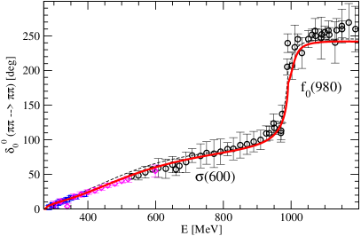
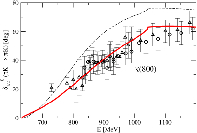
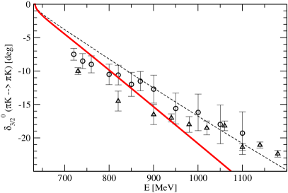
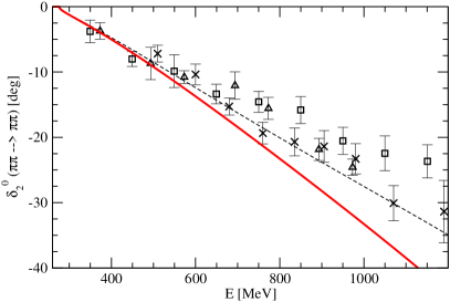
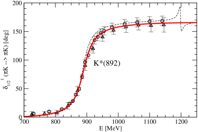
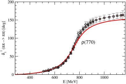
Figure 1: Solution for the meson-meson interaction [(red) solid lines]. For comparison, the results of ref. Oller:1998hw are shown with the dashed lines. Data: for $\delta_{0}^{0}$: (pink) diamonds Froggatt:1977hu , (blue) squares Batley:2007zz , (black) circles: average as defined in ref. Oller:1998zr ; for $\delta_{1/2}^{0}$: circles Aston:1987ir , triangles up: average as defined in ref. Oller:1998zr ; for $\delta_{3/2}^{0}$: circles Linglin:1973ci , triangles up Estabrooks:1977xe ; for $\delta_{2}^{0}$: crosses Rosselet:1976pu , squares Schenk:1991xe , triangles up Janssen:1994wn ; for $\delta_{1/2}^{1}$: triangles up Mercer:1971kn , circles Estabrooks:1977xe ; for $\delta_{1}^{1}$: squares Estabrooks:1974vu , circles Lindenbaum:1991tq .

The agreement of the solution of ref. Oller:1998hw (dashed lines in fig. 1) with the phase shift data is remarkable, except for the combination of isospin, angular momentum, strangeness $(I,L,S)=(1/2,0,-1)$, i.e. precisely the quantum numbers of the $\kappa(800)$ we are interested in. Thus, we have performed a refit to the data shown in figure 1 (i.e. from the respective thresholds up to $E=1.2$ GeV), with details given in the following: the $\kappa(800)$ channel is included in the $\chi^{2}$ with a special weight of 7. The pole position $z_{0}$ of the $\sigma(600)$ in the $(I,L,S)=(0,0,0)$ channel has been determined very precisely and model-independently in ref. Caprini:2003ta , $z_{0}=(441\pm i\,272)$ MeV. Thus, we simply consider this value as an additional data point that is included in the $\chi^{2}$, with an artificial error of $|\Delta z_{0}|=30$ MeV. While the data in the $\kappa$ channel are included with an increased weight, the $\chi^{2}$’s from the repulsive $I=2$ $\pi\pi$ and the $I=3/2$ $\pi K$ channels are included with a weight of $0.2$, while the data from the $\rho$ channel enter only with a weight of $0.1$ (note the data in that channel are quite precise). The value of the low-energy constant $L_{3}$ is particularly sensitive to the $\rho(770)$-channel and has been fixed in the fit to reproduce the bulk features of this resonance. With these trade-offs to achieve a better data description in the $\kappa(800)$ channel, the fit was performed, paying special attention to avoid spurious poles in the solution — the inverse amplitude method in the form used here is, to some extent, prone to generating narrow poles that are not physical. An example, from the solution of ref. Oller:1998hw , is visible in the dashed line in figure 1, for the $\delta_{1/2}^{1}$ phase at higher energies. In the present fit, such solutions were discarded.

The result of the fit is shown by the (red) thick solid lines in figure 1. In figure 2 the performance of the present fit is compared to additionally available data that were, however, not included in the $\chi^{2}$.

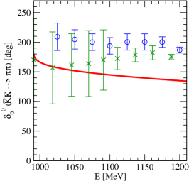
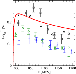
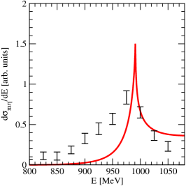
Figure 2: Further results (red (solid) lines; data not included in $\chi^{2}$) for the $(ILS)=(0,0,0)$ sector [$f_{0}(980)$ meson] (left and center panel) and for the $\pi\eta$ distribution [$a_{0}(980)$ meson] (right panel). Data: left and center: diamonds Froggatt:1977hu , crosses (X) Martin:1979gm , circles Cohen:1980cq , triangles Etkin:1981sg , squares Lindenbaum:1991tq ; right: ref. Armstrong:1991rg , background from there incoherently subtracted, see ref. Oller:1998zr .

Part of the data enter the $\chi^{2}$ with a weight different from one, and there is not much sense in calculating the reduced $\chi^{2}$, but the quality of the fit is obviously good, in particular in the $\kappa(800)$ channel. The trade-off paid for this agreement, visible in the $\rho(770)$ and the repulsive $\pi\pi$, $\pi K$ channels, is relatively small.

The values for the low-energy constants and $q_{\rm max}$ (the cut-off in the loop function $G$ Oller:1998hw ) are shown in table 1. These numbers are similar to those of ref. Oller:1998hw and also of the same order as they arise in CHPT, although there is no need for them to be precisely equal to a standard CHPT calculation due to a different fitted data range and conceptual differences to a full ${\cal O}(p^{4})$ calculation.

$L_{1}$	$L_{2}$	$L_{3}$	$L_{4}$ [t]
$0.873^{+0.017}_{-0.028}$	$0.627^{+0.028}_{-0.014}$	$-3.5$ [fixed]	$-0.710^{+0.022}_{-0.026}$ [b]
$L_{5}$	$L_{6}+L_{8}$	$L_{7}$	$q_{\rm max}$ [MeV] [t]
$2.937^{+0.048}_{-0.094}$	$1.386^{+0.026}_{-0.050}$	$0.749^{+0.106}_{-0.074}$	$981$ [fixed] [b]

Table 1: Fitted values for the $L_{i}$ [$\times 10^{-3}$] and $q_{\rm max}$ [MeV] with their uncertainties. As mentioned in the text, $L_{3}$ and $q_{\rm max}$ have been fixed in the determination of the error.

In addition, the non-linear parameter errors of the fit were determined and are also quoted in table 1. These errors are only indicative, because there are data in the fit that were included in the $\chi^{2}$ with weights different from one; the parameter errors are probably considerably larger than those quoted in table 1. Also, in the determination of the error, $L_{3}$ and $q_{\rm max}$ needed to be fixed. Otherwise, too large parameter correlation would have inhibited the determination of the error using the usual $\chi^{2}_{\rm best}+1$-criterion, where $\chi^{2}_{\rm best}$ is the $\chi^{2}$ at its minimum. Apart from this, the errors indicate that the low-energy constants can be well constrained from the data.

The resulting pole positions and residues are shown in table 2.

$I$	$L$	$S$	Resonance	sheet	$z_{0}$ [MeV]		$a_{-1}$ [$M_{\pi}$]		$a_{-1}$ [$M_{\pi}$]
$0$	$0$	$0$	$\sigma(600)$	$pu$	$434$	$+i\,261$	$-31$	$-i\,19\,(\bar{K}K)$	$-30$	$+i\,86\,(\pi\pi)$ [t]
				$uu$	$[411$	$+i\,233]$	$[0.2$	$-i\,0.2\,(\bar{K}K)]$	$[-29$	$+i\,42\,(\pi\pi)]$
$0$	$0$	$0$	$f_{0}(980)$	$pu$	$1003$	$+i\,15$	$16$	$-i\,79\,(\bar{K}K)$	$-12$	$+i\,4\,(\pi\pi)$
$1/2$	$0$	$-1$	$\kappa(800)$	$pu$	$815$	$+i\,226$	$-36$	$+i\,39\,(\eta K)$	$-30$	$+i\,57\,(\pi K)$
				$uu$	$[804$	$+i\,103]$	$[-0.4$	$+i\,15\,(\eta K)]$	$[-0.1$	$+i\,34\,(\pi K)]$
$1$	$0$	$0$	$a_{0}(980)$	$pu$	$1019$	$-i\,4$	$-10$	$-i\,107\,(\bar{K}K)$	$21$	$-i\,31\,(\pi\eta)$
$0$	$1$	$0$	$\phi(1020)$	$p$	$976$	$+i\,0$	$-2$	$+i\,0\,(\bar{K}K)$	—
$1/2$	$1$	$-1$	$K^{*}(892)$	$pu$	$889$	$+i\,25$	$-10$	$+i\,0.1\,(\eta K)$	$14$	$+i\,4\,(\pi K)$
				$uu$	$[915$	$+i\,22]$	$[-6.4$	$+i\,0.1\,(\eta K)]$	$[12$	$+i\,3\,(\pi K)]$
$1$	$1$	$0$	$\rho(770)$	$pu$	$755$	$+i\,95$	$-11$	$+i\,2\,(\bar{K}K)$	$33$	$+i\,17\,(\pi\pi)$
				$uu$	$[791$	$+i\,80]$	$[-7$	$+i\,1\,(\bar{K}K)]$	$[27$	$+i\,13\,(\pi\pi)]$ [b]

Table 2: Pole positions $z_{0}$ [MeV] and residues $a_{-1}[M_{\pi}]$ in the global fit to meson-meson observables. $I,\,L,\,S$ denote isospin, angular momentum, and strangeness, respectively. For the sheets, e.g. pu means physical (unphysical) sheet for the channel with higher (lower) threshold, in order. Values in brackets refer to poles that should not be compared to PDG values, because they are on hidden sheets. For the residues, e.g. $(\pi K)$ means the residue of $T(E)$ of eq. (1), of the $\pi K\to\pi K$ transition. Note that for the poles in the lower half plane, $a_{-1}(z_{0}^{*})=a_{-1}^{*}(z_{0})$.

If there is more than one entry for a resonance, the one without brackets corresponds to the standard sheet that is considered for the resonance. For example, the $\sigma(600)$ resonance is on the physical sheet with respect to the heavier $\bar{K}K$ channel, but on the unphysical one with respect to the lighter $\pi\pi$ channel, i.e. on the $pu$ sheet. The $uu$ sheet with the other pole of the $\sigma$ is far away from the physical axis at the $\sigma$ energies. For a general discussion of the analytic structure in hadron-hadron scattering, see, e.g., ref. Doring:2009yv . The $a_{0}(980)$ is special because its pole is on the $(pu)$ sheet, but at an energy above the $\bar{K}K$ threshold. This means the closest point of the physical axis to this pole is the $\bar{K}K$ threshold itself, which indeed shows a pronounced cusp in the $\pi\eta$ invariant mass spectrum as shown in figure 2. In the solutions of refs. Oller:1997ti ; Oller:1998hw the situation of the $a_{0}(980)$ pole is qualitatively the same. The role of threshold cusps and the possibility to disentangle their structure from lattice levels has been discussed in ref. Doring:2011vk .

The pole position of the $\sigma(600)$ shown in table 2 is close to the value extracted in the dispersive analysis of ref. Caprini:2003ta which is not a surprise as that pole position is included in the $\chi^{2}$. The pole position of the $K^{*}(892)$ is very close to the value quoted in PDG Nakamura:2010zzi . This is important as the main objective of this study is the $(\eta K,\,\pi K)$ system.

We would finally like to stress that in the presently considered UCHPT approach the considered channel space is limited to the two-body channels of scalar mesons. Multi-meson states or channels with (axial) vector particles are omitted, mostly because there is no phenomenological requirement for their inclusion at the energies of interest. The finite volume structure of multi-meson states is considerably more complicated than the two-body case considered here, and beyond the scope of this study.

2.1 Predicted lattice levels in the meson-meson sector

The discretization of the loop integral $G$ in eq. (1) generates the finite volume effects. In ref. Doring:2011vk , the discretized meson-meson loop function for $S$-waves has been derived with the result

$$\tilde{G}_{j} = \tilde{G}_{S,j}+\left(G_{j}-G_{S,j}\right)\ ,$$

$$\tilde{G}_{S,j} = \frac{1}{L^{3}}\sum_{\mathbf{n}}\,f_{j}(|\mathbf{q}|)\,F(q)\ ,\quad G_{j}=\int\limits^{|\mathbf{q}_{\rm max}|}\frac{d^{3}\mathbf{q}}{(2\pi)^{3}}\,f_{j}(|\mathbf{q}|)\ ,\quad G_{S,j}=\int\frac{d^{3}\mathbf{q}}{(2\pi)^{3}}\,f_{j}(|\mathbf{q}|)\,F(q)\ ,$$

$$\mathbf{q} = \frac{2\pi}{L}\,\mathbf{n},\,\,\,\mathbf{n}\in\mathds{Z}^{3}\ ,\quad f_{j}(q)=\frac{1}{2\omega_{j,1}(q)\,\omega_{j,2}(q)}\,\,\frac{\omega_{j,1}(q)+\omega_{j,2}(q)}{E^{2}-(\omega_{j,1}(q)+\omega_{j,2}(q))^{2}[+i\epsilon]}$$ (2)

with $\omega_{j,i}=\sqrt{M_{i}^{2}+|\mathbf{q}|^{2}}$, $M_{i}$ the masses of the two mesons in channel $j$, and $F$ is a form factor introduced in ref. Doring:2011vk to avoid artefacts ($e^{-M_{\pi}\,L}$ effects) from the sharp cut-off at $\mathbf{q}_{\rm max}$. The function $\tilde{G}_{j}$ is independent of this form factor, and $\tilde{G}_{S,j}-G_{S,j}$ can be rewritten in terms of the ${\cal Z}_{00}$ function Doring:2011vk up to relativistic effects that are of order $e^{-M_{\pi}\,L}$. As has been studied in ref. Doring:2011vk , the relativistic effects provided by eq. (2) can become significant. Up to the same $e^{-M_{\pi}\,L}$ effects the present discretization procedure is equivalent to the $K$-matrix formulation derived in ref. Bernard:2010fp . Note also that in the extraction of the scattering phase, in the one-channel case only the combination $\tilde{G}_{j}-G_{j}$ enters that is independent of the used form factor and cut-off at $\mathbf{q}_{\rm max}$ Doring:2011vk .

The lattice levels are obtained from the singularities of eq. (1) with the discretized $\tilde{G}_{j}$,

$$\det|V_{2}-V_{4}-V_{2}\,\tilde{G}\,V_{2}|=0,\quad\tilde{G}={\rm diag}\,(\tilde{G}_{1},\tilde{G}_{2})$$ (3)

where $\tilde{G}$ is a diagonal matrix in channel space that has two dimensions for the cases $(I,L,S)=(0,0,0),\,(1,1,0)$ [$\bar{K}K$, $\pi\pi$ channels], $(I,L,S)=(1/2,0,-1),\,(1/2,1,-1)$ [$\eta K$, $\pi K$ channels], and for $(I,L,S)=(1,0,0)$ [$\bar{K}K$, $\pi\eta$ channels]. Only one channel is present for the cases $(I,L,S)=(3/2,0,-1)$ [$\pi K$ channel], $(I,L,S)=(2,0,0)$ [$\pi\pi$ channel], and $(I,L,S)=(0,1,0)$ [$\bar{K}K$ channel], in which case eq. (3) is one-dimensional with $\tilde{G}=\tilde{G}_{j}$.

For the $P$-wave states, one has to complement eq. (2) with the corresponding angular momentum structure for the vertices, as spherical symmetry is broken on the lattice. In the general case of particles with spin $s_{1},\,s_{2}$ coupling to a total spin $S$, the angular structure $\gamma$ of a vertex that couples spin $(S,m)$ and orbital angular momentum $(\ell,M-m)$ to a total $(J,M)$ is

$$\gamma_{\boldsymbol{\alpha}}={\cal C}(S,\ell,J;m,M-m,M)\,Y_{\ell,m-M}(\theta,\phi)\,(-1)^{M-m}\\$$

with the Clebsch-Gordan coefficients ${\cal C}$ and $\boldsymbol{\alpha}=(J,M,\ell,S,m,\theta,\phi)$ abbreviates the quantum numbers and polar and azimuthal angles $\theta\in[0,\pi]$ and $\phi\in[0,2\pi]$. Note that the angles depend on the discretized momenta,

$$\theta=\arccos\frac{n_{z}}{\sqrt{n_{x}^{2}+n_{y}^{2}+n_{z}^{2}}},\quad\phi=\arctan(n_{y}/n_{x})$$ (4)

with $\mathbf{n}=(n_{x},n_{y},n_{z})\in\mathds{Z}^{3}$. For the present case of spinless meson-meson scattering in $P$-wave,

$$\gamma^{*}_{\boldsymbol{\alpha}}\gamma_{\boldsymbol{\alpha^{\prime}}}=3\,\cos^{2}\theta$$ (5)

and, thus, eq. (2) becomes

$$\tilde{G}_{S,j}^{\rm P-wave}=\sum_{\mathbf{n}}\,\gamma^{*}_{\boldsymbol{\alpha}}\gamma_{\boldsymbol{\alpha^{\prime}}}\,f_{j}(|\mathbf{q}|)\,F(q)=\tilde{G}_{S,j}\ ,{\rm i.e.},\ \tilde{G}_{j}^{\rm P-wave}=\tilde{G}_{j}\ .$$ (6)

The equation also indicates that for the special case of $P$-wave, the $\tilde{G}_{j}^{\rm P-wave}$ function is the same as for $S$-wave, $\tilde{G}_{j}$, given in eq. (2) . An analog situation has been found for the mass shift of bound states in a box in refs. Konig:2011nz ; Koenig:2011ti . This is no longer the case for $D$- and higher waves. Note also that sums $\sum_{\mathbf{n}}$ with an $S$-wave and a $P$-wave vertex disappear, i.e. there is no mixing of $S$- and $P$-waves. As is well known, there is mixing of $S$- and $G$-waves, and of $P$- and $F$-waves, but this is not an issue in the present study because the respective higher partial waves are small and, anyway, not generated from the NLO-terms used in this study.

With the $\tilde{G}$ function derived for $S$- and $P$-waves, and using the LO potentials $V_{2}$ and NLO potentials $V_{4}$, with the low-energy constants of the fit of table 1, eq. (3) can now be solved for its tower of zeros and at different box sizes $L$. The results are shown in figure 3 for the eight considered reactions.

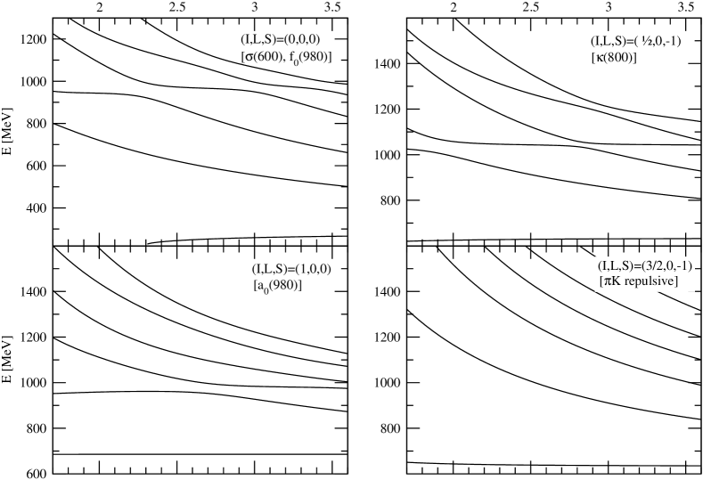
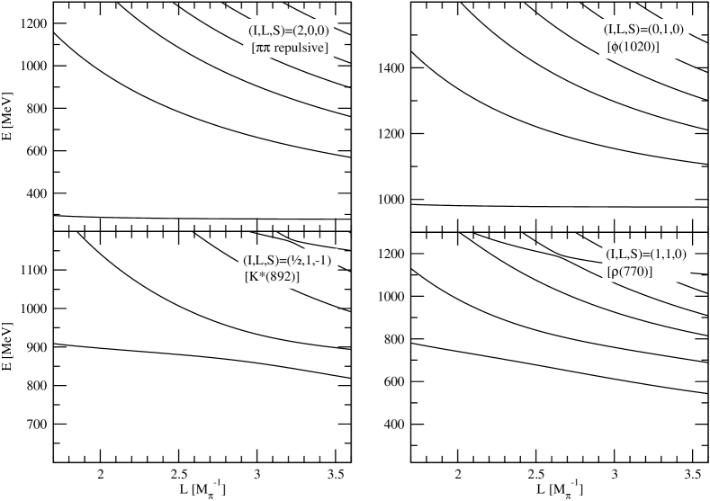
Figure 3: The first few levels for the considered reactions as calculated from the present solution for meson-meson scattering. Also, the corresponding resonances are indicated.

For the $(I,L,S)=(0,0,0)$ case, one can perceive the avoided level crossing around $E=990$ MeV that comes from a combined effect of the $\bar{K}K$ threshold and the $f_{0}(980)$ resonance located there. The situation of resonances close to thresholds and methods to extract those resonances from lattice data, e.g. by using twisted boundary conditions, have been discussed in refs. Bernard:2010fp ; Doring:2011vk . A similar situation is also given for the $a_{0}(980)$ [cf. figure 3] although in this case the resonance pole is considerably hidden on the $pu$ sheet in the present solution, see table 2. Also in case of the $\kappa(800)$ quantum numbers, shown to the upper right in figure 3, avoided level crossing is visible, coming in this case solely from the $\eta K$ threshold, as the $\kappa$ resonance pole is at lower energies. For the $P$-wave cases of the $K^{*}(892)$ and $\rho(770)$ quantum numbers, avoided level crossing is visible at higher energies $E>1.1$ MeV. This is due to the first free level of the higher channel, i.e. $\eta K$ for the $K^{*}(892)$ and $\bar{K}K$ for the $\rho(770)$ quantum numbers. As these channels couple very weakly to the dominant $\pi K$ and $\pi\pi$ channels, respectively, the crossing is almost ideal, i.e. the different levels come very close at the crossing energy. Note that, in contrast to $S$-wave channels, there is no avoided level crossing at the respective higher thresholds for the $P$-wave reactions, nor is there a lowest level close to the lower thresholds. An exception is given for the $\phi$-channel, but there the level at $E\sim 980$ MeV arises from the $\phi(1020)$ resonance that is just below the $\bar{K}K$ threshold, cf. table 2. The explanation for these findings is postponed until section 3.4.

For the $\kappa(800)$ channel, around the energy of the resonance, there is no structure visible in the levels shown in figure 3, and the same applies to the $\sigma(600)$. For the latter case, already studied in ref. Doring:2011vk , it is known that the $\sigma(600)$ pole can still be reconstructed, even if its position far in the complex plane results in a totally washed-out avoided level crossing. The situation should be similar for the $\kappa(800)$, and this question is addressed in section 3.

It should be noted that in the present approach we consider the finite volume effects on the meson-meson interaction, but do not attempt to determine finite size effects on the lattice levels. A comprehensive treatment of such systematic uncertainties would require to address the actual lattice action that generates the levels, but that goes far beyond the scope of the present study.

3 Reconstructing the $\boldsymbol{\kappa(800)}$

3.1 A suitable potential for resonance extraction

In the one-channel case, the Lüscher formalism provides a model-independent connection between phase shift (in the infinite volume limit) and lattice levels Luscher:1986pf ; Luscher:1990ux ; Luscher:1991cf . For the extraction of scattering lengths, see, e.g., also refs. Lage:2009zv ; Beane:2003da . In the two-channel case (see, e.g., ref. Lage:2009zv ), phase shifts, poles and residues can still be reconstructed model-independently provided three independent measurements of lattice levels at the same energy, to determine the channel transitions $V_{11}$, $V_{12}$, and $V_{22}$. This information can be obtained, e.g., from twisted boundary conditions or using spatially asymmetric boxes, as pointed out in refs. Bernard:2010fp ; Doring:2011vk .

However, if lattice data are provided with finite accuracy —present-day lattice simulations do not provide data for more than a few volumes, and with rather large error bars— the reconstruction of the infinite volume limit becomes a challenging task. A possible way of proceeding is to expand a general scattering potential $V$ in powers of the scattering energy, in one or more channels. The expansion parameters are then fitted to the lattice levels, and with the same potential $V$ the infinite volume limit can be recovered. Even broad resonances like the $\sigma(600)$ or resonances close to a threshold like the $f_{0}(980)$ can be reconstructed as shown in ref. Doring:2011vk .

The two-channel fit potential used in ref. Doring:2011vk is given by

$$V_{ij}=a_{ij}+b_{ij}(s-4M_{K}^{2})\,$$ (7)

where $i,j=1,2$ indicate the channel. The six parameters $a_{ij}=a_{ji},\,b_{ij}=b_{ji}$ provide an expansion up to terms linear in $s=E^{2}$, with the expansion point $s_{0}=4M_{K}^{2}$ at the $\bar{K}K$ threshold that is suitable for the study of the $f_{0}(980)$ resonance since the parameter correlations are minimized. The problem at hand in ref. Doring:2011vk is specially suited for the choice of the fit potential shown in eq. (7), because the LO chiral interaction in the $(\bar{K}K,\,\pi\pi)$ system depends only linearly on $s$. If then pseudo-data, generated from the very interaction, are fitted with the ansatz of eq. (7), ideally a $\chi^{2}$ of zero can be obtained. In the present case of the $(\eta K,\,\pi K)$ system, the LO interaction depends already on $s$ and $t$, and the NLO terms have $s^{2}$-, $t^{2}\,\cdots$-dependence. A possible refinement of the potential $V$ could, thus, be an expansion not only in $s$ but also in $t$,

$$V_{ij}=a_{ij}+b_{ij}(s-s_{0})+b^{\prime}_{ij}(t-t_{0})+c_{ij}(s-s_{0})^{2}+\cdots\,\ .$$ (8)

The dependence on the Mandelstam variable $u$ can be expressed in this ansatz by $s$, $t$ and a constant, and terms $\sim(u-u_{0})$ should not be included explicitly. One should note that in $S$-wave, terms proportional to $t$ are to a good approximation linear functions of $s$, and large correlations between $a,b,b^{\prime}$ appear. It is then more efficient to absorb the $t$-dependence in the parameter $b$, and also in $c$ for the small order-$s^{2}$ differences between $s$ and $t$.

As we have just seen, in the presence of terms $\sim t$ and higher order terms from NLO, a quadratic term of the form $(s-s_{0})^{2}$ is indispensable in the expansion of the fit potential. This will, of course, introduce additional free parameters in the fit potential. Together with the fact that only very few data points are available in actual lattice simulations, there will still be large parameter correlations and, worse, the fit will have too much freedom in between those data points and generate solutions that have a good $\chi^{2}$ but should not be accepted because the natural hierarchy of the expansion is no longer given —e.g., the term $\sim(s-s_{0})^{2}$ may be unnaturally large compared to the terms $(s-s_{0})^{1}$ and $(s-s_{0})^{0}$. The situation can be improved by providing the expansion the well-defined, model-independent LO term of the chiral expansion. This term almost saturates the constant and the linear parameters $a$ and $b$, and thus considerably stabilizes the fit. Remaining contributions to $a$ and $b$ will then be much smaller, and the above-mentioned, unnatural solutions are automatically avoided.

The question is in which form to cast the resulting fit potential. For a resonance analysis, the inverse amplitude method itself is particularly suited because the organization of the LO and NLO potentials, $V_{2}$ and $V_{4}$, allows for solutions in which resonance terms can be expressed in terms of the $V_{2}$, $V_{4}$ Oller:1998hw . Thus, this form of the parameterization is quite flexible, and we choose it for the final form of the fit potential used throughout this study. The finally adopted form of the fit potential reads in the one-channel case

$$V^{\rm fit}=\left(\frac{V_{2}-V_{4}^{\rm fit}}{V_{2}^{2}}\right)^{-1},\quad V_{4}^{\rm fit}=a+b(s-s_{0})+c(s-s_{0})^{2}+d(s-s_{0})^{3}+\cdots$$ (9)

with $V_{2}\equiv V_{\rm LO}$ the fixed LO term of the chiral expansion. In other words, we take the form of the inverse amplitude, leaving the LO term $V_{2}$ as it is, and expand $V_{4}$ in powers of $s$. The $T$ matrix in the infinite volume limit is then obtained as

$$T=\frac{1}{(V^{\rm fit})^{-1}-G},\quad{\rm i.e.,}\quad T=V^{\rm fit}+V^{\rm fit}\,G\,T~{},$$ (10)

and the lattice levels are given through the condition

$$(V^{\rm fit})^{-1}-\tilde{G}=0\quad\leftrightarrow\quad V_{2}-V_{4}^{\rm fit}-V_{2}^{2}\tilde{G}=0$$ (11)

where $\tilde{G}=\tilde{G}_{\pi K},\,G=G_{\pi K}$ from eq. (2) for the $\kappa(800)$ channel. In the present study, we do not generalize this fit potential to two channels. The pseudo-data which will be fitted are, of course, generated from the full two-channel solution obtained in the previous section. The $\kappa(800)$ is situated well below the $\eta K$ threshold, and the influence from the $\eta K$ channel should be noticed, at most, as a small perturbation that can be absorbed in the fit potential. Note in this context that the pseudo-phase Bernard:2010fp in the $(\bar{K}K,\,\pi\pi)$ system is very close to the true phase up to a few MeV below the $\bar{K}K$ threshold Doring:2011vk . In any case, these arguments will be tested in the following: if no good fits could be obtained, the one-channel extraction method would lead to erroneous phase shifts and pole positions.

As the LO chiral interaction $V_{2}$ enters the fit potential explicitly to stabilize the solution, the question arises to which extent extracted pole positions are biased: for example, $V_{2}$ alone already generates poles in $S$-wave that can be identified with the $\sigma(600)$, $f_{0}(980)$, and $a_{0}(980)$ resonances Oller:1997ti . This is also the case for the $\kappa(800)$ resonance. However, note that $V_{4}^{\rm fit}$ in eq. (9) contains also terms $\sim s^{0}$ and $\sim s^{1}$ as they appear in $V_{2}$. Thus, $V^{\rm fit}$ is sufficiently general to modify the fixed LO contribution, and resonances may or may not appear in the reconstruction process, as dictated by the lattice data themselves. This provides a much more model-independent approach to the extraction of the finite volume limit as it would be the case by making assumptions on the resonance propagator as, e.g., in refs. Gockeler:2008kc ; Feng:2010es ; Lang:2011mn ; Fu:2011xw .

Finally, it is worthwhile noting that the proposed one-channel extraction method is entirely independent of the used regularization scheme because only the difference $\tilde{G}_{j}-G_{j}$ appears in the connection between the $T$-matrix in the infinite-volume limit and the lattice levels, eqs. (10) and (11).

3.2 Extraction of the $\boldsymbol{\kappa(800)}$

Fitting pseudo-data with the potential of eq. (9) allows to study the propagation of the uncertainty from the lattice to the quantities of interest, i.e., the phase shift and the $\kappa(800)$ pole position in the infinite volume limit. To generate the pseudo-data, we consider the levels as shown in figure 3 to the upper right. The possible pole position is expected around $E\sim 650-850$ MeV, but at the values of $L$ shown in the figure, which are values that can be covered in actual lattice simulations, there is no level at these energies. Still, one can choose the nearby level at the $\pi K$ threshold and the following one, without getting too close to the $\eta K$ threshold. In principle, one could include also data from the $\eta K$ threshold region, generalizing the fit potential of eq. (9) to two channels. However, in actual lattice simulations only few data will be available and the number of free parameters in the two-channel potential would be three times larger, most of them being weakly constrained (the ones from the $V_{\eta K\to\eta K}$ and $V_{\pi K\to\eta K}$ transitions). This would, thus, be a poor strategy to study the $\kappa(800)$.

Given these arguments, the finally chosen pseudo-data from the levels of figure 3 are shown in figure 4 to the left.

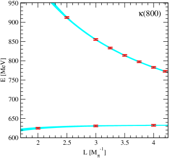
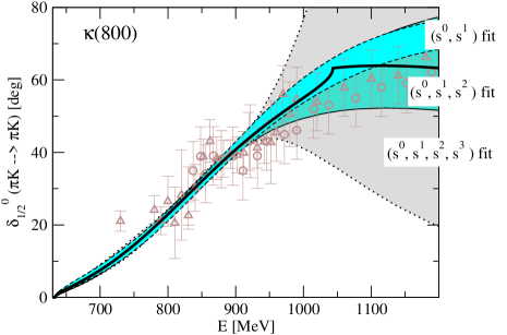
Figure 4: Left: Pseudo lattice-data and ($s^{0},\,s^{1},\,s^{2}$) fit to those data with uncertainties (bands). Right: Solid line: Phase shift of the solution that was used to generate these pseudo lattice-data. Also, the resulting error bands of the $(s^{0},\,s^{1})$, $(s^{0},\,s^{1},\,s^{2})$, and $(s^{0},\,s^{1},\,s^{2},\,s^{3})$ fits to these data are shown.

A constant error of $2$ MeV is assigned to each data point, but we will also study the case of a 5 MeV error. In ref. Doring:2011vk the additional error, induced by the statistical displacement of the centroids of the error bars, has been studied. Displacing the centroid according to a Gauss distribution with half the width of the error bars themselves, the uncertainties of extracted phase shifts and pole positions were found to be enlarged by $\sim 40$%. We will not repeat this exercise in the analyses of this work, but one should keep in mind additional errors of this size on the extracted quantities.

Using eqs. (9) in eq. (11), the fit is performed at an expansion point of $s_{0}=~{}(750\,{\rm MeV})^{2}$ in eq. (9). Depending on the power to which the fit potential is expanded, the fits are labeled $(s^{0}),\cdots,\,(s^{0},\,s^{1},\,s^{2},\,s^{3})$ in the following. Error bands are generated by accepting all solutions for which $\chi^{2}\leq\chi_{\rm best}^{2}+1$ where $\chi^{2}_{\rm best}$ is the $\chi^{2}$ of the best fit. The error bands for the levels themselves, from the ($s^{0},\,s^{1},\,s^{2}$) fit, are shown in figure 4 in the left panel, and for the phase shift to the right. Also, to the right, the solid line shows the phase shift of the solution that was used to generate the pseudo lattice-data, which lies, as expected, in the center of the error bands up to $E\sim 900$ MeV while it deviates at higher energies. This is because, first, no lattice data are fitted beyond $E\sim 920$ MeV, and second, the solution to generate the data is formulated in the full two-channel approach while the fit potential is in one channel only. This manifests itself in a cusp of the full solution at the $\eta K$ threshold, while the extracted phase shifts are smooth there. As the figure shows, fits with higher power in the fit potential show a larger spread of possible phase shifts at higher energies. This is expected because more free parameters in the fit potential lead to a better fit of the level, but also and unavoidably, to a wider error band.

The next question is to which precision the pole position of the $\kappa(800)$ can be determined. The main problem is the large width of this resonance —small uncertainties on the real, physical axis at ${\rm Im}~{}E=0$ MeV result in large uncertainties far in the complex plane. In figure 5 the pole positions as extracted from the pseudo lattice-data are shown for the different fit functions. The central values are indicated with the symbols while the areas show the corresponding uncertainties.

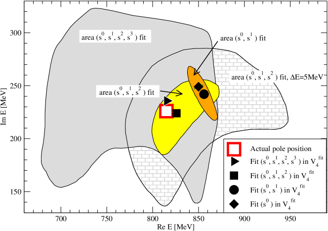
Figure 5: Pole reconstruction of the $\kappa(800)$. The actual pole position is obtained from a global fit to meson-meson scattering data, cf. table 2. Shown are the pole positions of the $\kappa$ with uncertainty areas as obtained from different fits to pseudo lattice-data. The lattice data carry an error of 2 MeV, except for the case $\Delta E=5$ MeV as specified in the figure.

As for the central values, the $(s^{0},\,s^{1},\,s^{2})$ and $(s^{0},\,s^{1},\,s^{2},\,s^{3})$ fits are close to the actual pole position, while the $(s^{0})$ and $(s^{0},\,s^{1})$ fits are not. This indicates that the $\sim s^{2}$ term in eq. (9) is important. As argued in the previous section, this term bears part of the $t$- and $u$-dependence of the potential, plus parts of the NLO interaction. Both turn out to important. Considering the uncertainty areas, we observe the same behavior as for the phase shifts: the areas grow with increasing number of fit parameters and higher powers in the potential. In particular, for the $(s^{0})$ and $(s^{0},\,s^{1})$ fits the areas are very small, giving the wrong impression of high precision but the areas do not cover the actual pole position. In contrast, the uncertainty area of the $(s^{0},\,s^{1},\,s^{2})$ and $(s^{0},\,s^{1},\,s^{2},\,s^{3})$ fits do cover the actual pole position.

While in our analysis of pseudo lattice-data the actual pole position is known, in the analysis of real lattice data it is not. Still, the previous observations lead to the formulation of a simple fit strategy:

1. The fit potential should be expanded to higher and higher powers in $s$.

2. Once the central value of the pole position does not change any more —here, given for the $(s^{0},\,s^{1},\,s^{2},\,s^{3})$ fit— one can assume convergence.

3. One can then use the previous fit to determine the uncertainty area —here given by the $(s^{0},\,s^{1},\,s^{2})$ fit and the yellow area in the plot. This can be regarded as the final result of the analysis.

The chosen data uncertainty of $2$ MeV is very small, and we show in figure 5 also the uncertainty area for a $5$ MeV error, for the $(s^{0},\,s^{1},\,s^{2})$ fit. This results in an error of around $\pm 90$ MeV for the real part of the pole position and around $\pm 75$ MeV for the imaginary part, i.e. $\pm 150$ MeV for the width. The residues of the extracted $\kappa(800)$ poles and of all other resonances analyzed in this study can be found in section 4.4.

3.3 Case of a low $\boldsymbol{\kappa(800)}$ pole

The pseudo-data analyzed in the previous section are based on the global fit to meson-meson scattering data carried out in section 2. The outcome for the real part of the $\kappa(800)$ pole position of $z_{0}=(815\pm i\,226)$ MeV is rather at the upper end of the pole positions quoted in the PDG Nakamura:2010zzi . To cover also low pole positions of the $\kappa(800)$, we repeat the analysis using a different solution for which we include, in the $\chi^{2}$ of the fit, one of the lowest pole positions quoted in the PDG Nakamura:2010zzi . The pole position is the result of the Roy-Steiner analysis of ref. DescotesGenon:2006uk with $z_{0}=(658\pm i\,278.5)$ MeV. For simplicity, we use only the $\pi K$ channel for the chiral unitary model and include, besides the $\kappa$ pole position, only the partial wave data from the $\pi K$ partial waves $(I,L,S)=(1/2,0,-1),\,(1/2,1,-1)$ up to $E=1.2$ GeV [see figure 1 for the data and their references]. The $\kappa$ pole position is included with a chosen error of $35$ MeV in the $\chi^{2}$. To constrain the low-energy constants, also $\pi\pi$ scattering data have been included in the $\chi^{2}$, but only to ensure the $\sigma(600)$ pole is still present. Furthermore, we have made sure that the fitted combination of low-energy constants leads to qualitatively correct solutions in the other meson-meson reactions.

The refit of the low-energy constants (except for $L_{7}$ that does not contribute in $\pi K\to~{}\pi K$) leads to a quantitative description of the data in the $\pi K$ partial waves $(I,L,S)=(1/2,0,-1),\,(1/2,1,-1)$. This is shown by the solid line in figure 6 in the right panel (the $K^{*}(892)$ channel is not shown again). The pole position at $z_{0}=~{}(679\pm~{}i\,~{}271)$ MeV is quite close to the fitted one of ref. DescotesGenon:2006uk and at the lower end of values quoted in the PDG Nakamura:2010zzi .

The fit solution provides the pseudo-data that are selected following the same arguments as in the previous section. The pseudo-data and the error bands of the corresponding ($s^{0},\,s^{1},\,s^{2}$) fit are shown in figure 6 to the left, applying the same $\chi_{\rm best}^{2}+1$-criterion as in the previous section. To the right, the error band of the extracted phase shift from the ($s^{0},\,s^{1},\,s^{2}$) fit is indicated with the filled (cyan) area.

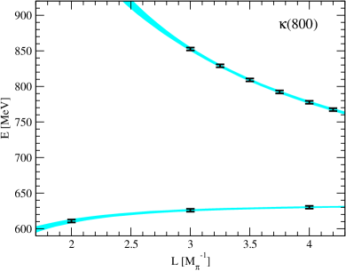
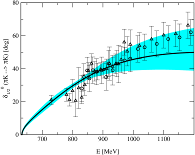
Figure 6: Case of a low $\kappa(800)$ pole. Left: Pseudo lattice-data and uncertainty of the $(s^{0},s^{1},s^{2})$ fit to those data (bands). Right: Solid line: Phase shift for the solution that was used to generate these pseudo lattice-data. Also, the resulting error band of the $(s^{0},s^{1},s^{2})$ fit to these data is shown.

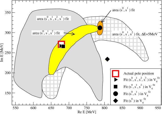
Figure 7: Case of a low $\kappa(800)$ pole. Pole positions of the $\kappa$ (central values) together with uncertainty areas, from fits to pseudo lattice-data. All symbols and areas are defined as in figure 5.

Comparing with the previous case of a higher $\kappa$-pole, shown in figure 4, the error bands both for levels and phase shifts are similar for the respective ($s^{0},\,s^{1},\,s^{2}$) fits.

In figure 7 the pole positions as extracted from the pseudo lattice-data are shown for the different fit functions, in full analogy to the results shown in figure 5. The central values are indicated with the symbols, the areas show the corresponding uncertainties. We can perceive the same behavior of the fits as in the previous case of a rather high $\kappa$-pole position: expanding the fit potential to too low powers, wrong central values are extracted in combination with too small uncertainty areas that give the impression of an unrealistic precision. Once also the $s^{2}$-term is fitted, the central value is close to the actual pole position. Including also the $s^{3}$-term in eq. (9) serves then to confirm the result of the $(s^{0},s^{1},s^{2})$ fit, because the central value is not changed any more and only the uncertainty area grows. The realistic uncertainty is then again given by the yellow shaded area from the $(s^{0},s^{1},s^{2})$ fit.

3.4 Qualitative analysis using the lowest level

In the previous sections we have seen that relatively precise lattice data are needed to pin down the pole position of the $\kappa(800)$. Still, one may wonder if with a few and low precision data points from the lowest level, which is the one that can be most precisely determined in actual lattice simulations, one can at least make qualitative statements about the presence, absence, and maybe approximate position of the pole.

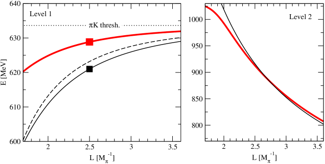
Figure 8: Levels 1 and 2. Thick (red) solid lines: case of higher pole position from section 3.2. Thin (black) solid lines: case of lower pole position from section 3.3. Dashed line: Approximation of eq. (13) for the case of lower pole position. The squares to the left indicate the measurements taken to calculate the approximations to phase shifts and pole positions shown in figure 9.

In figure 8 the levels 1 and 2 are shown. The case of a higher $\kappa(800)$ pole position [cf. section 3.2] is indicated with the thick (red) solid line, the case of lower pole position [cf. section 3.3] with the thin (black) solid line. As the figure shows, the largest differences of the two solutions are visible for level 1, and those differences are enhanced to more than 10 MeV for the smallest $L$. In contrast, level 2 shows only differences of a few MeV below $E\sim 900$ MeV. In the following, we will study to which extent the low-$L$ enhancement of level 1 can help to draw qualitative conclusions on the $\kappa(800)$ pole.

We start with the derivation of an approximate expression for the $L$-dependence of the first level. In the present formulation the function $\tilde{G}$ of eq. (2) can be expanded in a Laurent series around the pole at threshold,

$$\tilde{G}=\frac{1}{4m_{1}\,m_{2}\,L^{3}}\,\frac{1}{E-(m_{1}+m_{2})}+{\cal O}[E-(m_{1}+m_{2})]^{0}\$$ (12)

where we can ignore contributions from $G$ and $G_{S}$ in eq. (2) of order ${\cal O}[E~{}-~{}(m_{1}+~{}m_{2})]^{1/2}$. For an $S$-wave interaction, we can approximate the potential $V$ close to threshold by a constant, $V^{\rm fit}=C_{\pi K}$. The levels are given by $1-V^{\rm fit}\tilde{G}=0$ (the problem can be reduced to one channel for this exercise), so that

$$E=m_{1}+m_{2}+\frac{C_{\pi K}}{4\,m_{1}\,m_{2}\,L^{3}}\ .$$ (13)

This is equivalent to the standard result for the scattering length, see refs. Luscher:1986pf ; Luscher:1990ux ; Beane:2003da . There will always be a level close to threshold with this functional behavior, because $\tilde{G}$ diverges at threshold and always equals $(V^{\rm fit})^{-1}$ for some $E$ close to it. In particular, we read from eq. (13) that if the interaction is attractive $(C_{\pi K}<0)$, the level will be slightly below threshold, while for $C_{\pi K}>0$ it will be above. For the $S$-wave, we observe exactly this behavior for all cases shown in figure 3. Note that once $C_{\pi K}$ is determined from lattice data using eq. (13), one can relate it to the scattering length. With the isospin $I=1/2$ $S$-wave scattering length defined as $\lim_{q_{\rm c.m.}\to 0}q_{\rm c.m.}\,\cot\delta_{1/2}^{0}=1/a_{1/2}^{0}$ and $a_{1/2}^{0}=-{\rm Re}\,T_{1/2}^{0}(E=M_{\pi}+M_{K})/[8\pi\,(M_{\pi}+M_{K})]$ in the current normalization of the amplitude $T$ we obtain

$$a_{1/2}^{0}=\frac{1}{8\pi\,E}\,\frac{C_{\pi K}}{C_{\pi K}\,G_{\pi K}-1}\bigg{|}_{E=M_{\pi}+M_{K}}\ .$$ (14)

Back to the original problem, the approximation of eq. (13) for level 1 is shown in figure 8 with the dashed line for the case of low $\kappa$ pole. The agreement is quite good. With $C_{\pi K}$ determined from eq. (13), we can exploit the fit potential of eq. (9). The measured $C_{\pi K}$ fixes the parameter $a$ of $V_{4}^{\rm fit}$, while $b,c,d$ are set to zero as they cannot be fixed,

$$V_{4}^{\rm fit}=V_{2}^{\rm thres.}\left(1-\frac{V_{2}^{\rm thres.}}{C_{\pi K}}\right)={\rm const.},\quad V_{2}^{\rm thres.}=V_{2}(s=(M_{\pi}+M_{K})^{2})\ .$$ (15)

Using eq. (10), phase shifts and pole positions may be determined now. For the numerical calculation, we have determined $C_{\pi K}$ by measuring the lowest level at $L=2.5M_{\pi}^{-1}$, as shown by the squares in figure 8, and then using eq. (13).

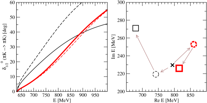
Figure 9: Dashed lines/dashed circles: Approximations of phase shifts (left) and pole positions (right) using only one data point from level 1 as shown by the squares in figure 8. For comparison, the full results are shown: Thick solid (red) line and thick (red) square: case of high $\kappa$ pole position. Thin solid (black) line and thin (black) square: case of low $\kappa$ pole position.

The result is shown in figure 9 for the two cases of higher and lower pole position. In the left panel, the actual phase shifts (solid lines) and the ones determined using eq. (15) are shown (dashed lines). Indeed, using only the information from the lowest level, encoded in $C_{\pi K}$, the phase can be qualitatively described, in particular for the case of a higher $\kappa$ pole. The pole positions are shown in the right panel of figure 9. The actual pole positions are indicated with the squares, the ones determined using eq. (15) are shown with the circles, and the pole position obtained when setting $V_{4}^{\rm fit}=0$, i.e. the pole position from the LO calculation (in one channel), is marked with the cross. Here, the situation is not as clear as for the phases. In particular, the approximations of the actual pole positions, given by the method proposed here (circles), show no systematic improvement compared to the case $V_{4}^{\rm fit}=0$ (cross). In summary, measuring $V_{4}^{\rm fit}$ at one $L$ using the lowest level improves the description of the phase close to threshold. However, beyond the threshold region, clearly the higher order terms $\sim s,\,s^{2}$ in $V_{4}^{\rm fit}$ need to be known to allow for a quantitative determination of the phase and the $\kappa$ pole.

To conclude this section, we come back to a question left open in the discussion of figure 3: why is there no level close to the lower thresholds of the $P$-wave reactions, while there is always one for the $S$-wave reactions? For $P$-waves, the potential close to threshold will be of the form $V=a^{\prime}\,q_{\rm c.m.}^{2}$ with a nearly constant $a^{\prime}$. Expanding $q_{\rm c.m.}$ as a function of $E$ one finds that the pole of $\tilde{G}$ (see eq. (12)) is precisely canceled in $1-V\tilde{G}=0$,

$$1-V\tilde{G}\sim 1-\frac{a^{\prime}}{2\,L^{3}\,(m_{1}+m_{2})}$$ (16)

and there is no need for this expression to become zero, i.e. no need for the occurrence of a level close to a $P$-wave threshold. The absence of avoided level crossing at the respective upper thresholds, for the $P$-wave channels, can be explained similarly.

4 Extraction of other excited meson states

To put the previous results on the $\kappa(800)$ into context, in particular the required high precision of the lattice data, in the following the $\sigma(600)$ is analyzed that has similar properties. Also, the results for these $S$-wave resonances are contrasted with the $P$-wave $K^{*}(892)$ and $\rho(770)$ states, as well as the repulsive $\pi K$ and $\pi\pi$ phase shifts.

4.1 The $\boldsymbol{\sigma(600)}$ at next-to-leading order

In the previous sections, lattice data with an error of $2$ MeV were required to obtain a sensible error on the pole position of the $\kappa(800)$, as shown with the (yellow shaded) $(s^{0},s^{1},s^{2})$-areas in figures 5 and 7. This result is in certain contrast with the pole reconstruction of the $\sigma(600)$ in ref. Doring:2011vk where a few data points with a $10$ MeV error were found enough to obtain a reasonable determination of the pole. We repeat the current analysis to put these differences into context. For this, we use the same values of $L$ as in ref. Doring:2011vk to generate 6 data points with a 10 MeV error . These data are fitted in a $(s^{0},\,s^{1})$ fit, like in ref. Doring:2011vk , with the result for the pole position and uncertainty (orange area) shown in figure 10 to the left.

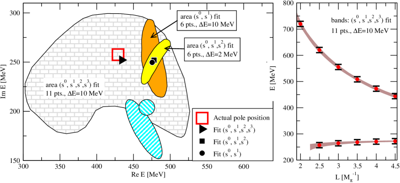
Figure 10: Left: Pole reconstruction of the $\sigma(600)$. The (black) symbols show different fits, the actual pole position is shown by the (red) open square. Uncertainty areas are labeled. For comparison, the result from ref. Doring:2011vk is shown with the hatched circle (pole position) and hatched uncertainty area, obtained from a $(s^{0},\,s^{1})$ fit. Right: 6 data points from the upper level (level 2) plus 5 points from level 1, as used for the fits. The data errors and uncertainty band for one fit is shown as indicated in the figure.

The corresponding result from ref. Doring:2011vk is shown with the hatched areas in figure 10. As the figure shows, for the present result and the one from ref. Doring:2011vk , the uncertainty is of quite similar size. However, the central value in the present case (filled circle) is quite far from the actual position: Like in the case of the $\kappa(800)$, there are now sizeable NLO terms $\sim~{}s^{2}$ that cannot be accommodated in a simple $(s^{0},\,s^{1})$ fit. Thus, to better reconstruct the original pole position of the $\sigma(600)$, we have performed an $(s^{0},\,s^{1},\,s^{2})$ fit, but with a $2$ MeV error for the data (yellow area). As the figure shows, the corresponding uncertainty area (yellow) is of similar size as for the case of the $\kappa(800)$ from Figs. 5 and 7. Concluding, in ref. Doring:2011vk a 10 MeV error on the data produces an uncertainty of similar size as $2$ MeV data errors here, because the fit potential here is expanded to higher powers. As figure 10 shows, even the $(s^{0},\,s^{1},\,s^{2})$ fit shows no agreement of the central value with the actual pole position. The $(s^{0},\,s^{1},\,s^{2},s^{3})$ fit, however, does. To minimize the uncertainty area for this case, in addition to the 6 points from level 2, 5 points from level 1 are included in the fit, that would be known in an actual lattice calculation anyway. As the figure shows, one can then provide again a 10 MeV error to the data to obtain a large, but still limited uncertainty area .

4.2 P-wave states: Extraction of the $\mathbf{K^{*}(892)}$ and the $\boldsymbol{\rho(770)}$

While the broad $\kappa(800)$ and $\sigma(600)$ $S$-wave resonances, discussed in the previous sections, require relatively precise lattice data, some $P$-wave resonances are expected to show clearer signals on the lattice: For $P$-wave the lowest lattice level —i.e. the most accessible one— is located already in the resonance region, in contrast to the $S$-wave that has a level at the lowest threshold (see figure 3 and section 3.4). Also, resonances like the $K^{*}(892)$ and $\rho(770)$ are much narrower than the analyzed $S$-wave states and the corresponding $\pi K$ and $\pi\pi$ channels show only very weak coupling to the respective $\eta K$ and $\bar{K}K$ channels Oller:1998hw , making the analysis easier than in case of, e.g., the $f_{0}(980)$ or $a_{0}(980)$ resonances Bernard:2010fp ; Doring:2011vk ; Doring:2011ip . Lattice calculations and resonance extraction at finite volume for the $\rho(770)$ have already allowed for a determination of its mass and the $\rho\pi\pi$ coupling constant, at a pion mass of around twice the physical one, see, e.g., ref. Lang:2011mn . The relativistic Breit-Wigner form, assumed in ref. Lang:2011mn , or effective range formulae assumed in refs. Gockeler:2008kc ; Feng:2010es , are adequate for the $\rho(770)$, but the method presented here is a more general model-independent extraction of the resonance properties.

The $S$-wave fit potential from eq. (9) can be generalized to $P$-wave with minor changes. Noting that the threshold behavior is given by $V^{\rm fit}_{P-{\rm wave}}\sim q_{\rm c.m.}^{2}$, we can simply multiply this factor to the $S$-wave potential to obtain

$$V^{\rm fit}_{P-{\rm wave}}=\left(\frac{V_{2}-V_{4}^{\rm fit}}{V_{2}^{2}}\right)^{-1},\quad V_{4}^{\rm fit}=q_{\rm c.m.}^{2}\left[a+b(s-s_{0})+c(s-s_{0})^{2}+\cdots\right]$$ (17)

and $V_{2}$ is given by the $P$-wave projected LO term.

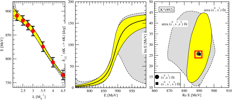
Figure 11: Extraction of the $K^{*}(892)$ resonance using 7 data points from level 1 with $10$ MeV error (left). Center and right: Phase shifts and pole position, respectively. The (yellow) areas show the uncertainty of the $(s^{0},s^{1})$ fit, the (gray) areas the one of the $(s^{0},s^{1},s^{2})$ fit. The actual phase [pole position] is indicated with the thick solid line [open (red) square]. The central values of the fitted pole position are indicated with the filled circle and the filled square.

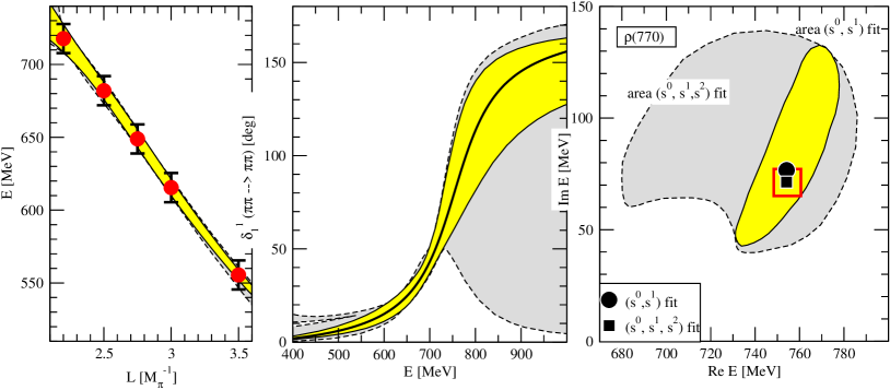
Figure 12: Extraction of the $\rho(770)$ resonance using 5 data points from level 1 with $10$ MeV error (left). Center and right: Phase shifts and pole position, respectively. Labeling as in figure 11.

For the generation of pseudo-data in the $(\eta K,\,\pi K)$ $P$-wave channel, the global solution determined in section 2 has been used, while for the pseudo-data of the $(\bar{K}K,\,\pi\pi)$ $P$-wave we use the solution of ref. Oller:1998hw that is slightly better for this quantum number (dashed vs. solid line in figure 1).

The analysis of the pseudo-data can be carried out as in the previous sections, with the result for the $K^{*}(892)$ shown in figure 11 and for the $\rho(700)$ in figure 12. For both resonances, the $(s^{0},s^{1})$ fits lead to pole positions very close to the actual ones, indicated with the open (red) squares. Note that contributions to the $s^{1}$-term in $P$-wave correspond, among others, to terms of the form $ts$, $us$, $t^{2}$, or $u^{2}$ as they appear in the NLO potential Oller:1998hw . The $(s^{0},s^{1},s^{2})$ fits return practically the same pole positions and much enlarged uncertainty areas. This indicates that the $(s^{0},s^{1})$ fits and their uncertainty areas can be regarded as the final results, according to the fit strategy formulated in section 3.2.

The observed convergence for $(s^{0},s^{1})$ fits should be seen in comparison to the previous results for the $S$-wave resonances: for the $\kappa(800)$, convergence occurs only for the $(s^{0},s^{1},s^{2})$ fit, while for the $\sigma(600)$ the potential needs to be expanded to even one more power. Thus, the properties of the considered $P$-wave resonances are indeed much easier to determine than their $S$-wave counterparts.

For the $K^{*}(892)$, seven data points up to values of $L=4.5\,M_{\pi}^{-1}$ have been fitted. As figure 11 shows, the (yellow) uncertainty area of the levels is broad at low $L$ and narrow at large $L$. This indicates that the data at small $L$ predominantly fix the fit result, while those at high $L$ may be dispensable. Thus, for the analysis of the $\rho(770)$ the two data points at $L>3.5\,M_{\pi}^{-1}$ were omitted as shown in figure 12. Indeed, the $\rho(770)$ properties could be determined to a similar quality as the ones of the $K^{*}(892)$, taking into account that the larger width of the $\rho(770)$ automatically leads to an enlarged uncertainty area.

Thus, the analysis of pseudo-lattice data can help to identify regions of the lattice spectrum that are particularly sensitive to resonance properties. Such findings can contribute to minimize the required effort of actual lattice calculations.

4.3 The $\boldsymbol{\pi K}$ and $\boldsymbol{\pi\pi}$ repulsive phase shifts

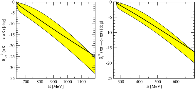
Figure 13: Extraction of the repulsive $\pi K$ (left) and $\pi\pi$ phase shifts (right). The thick solid lines show the actual phase shifts. The (yellow) bands show the extracted phase shifts using one data point of the respective lowest level, at $L=2.5\,M_{\pi}^{-1}$ and with a $10$ MeV error.

To put the resonance analyses of the previous sections into context, we apply the same method to phase shifts without resonances. The repulsive $\pi K$ isospin $3/2$ and $\pi\pi$ isospin $2$ phases show no structure and an almost linear energy dependence. As the $\pi\pi$ isospin $2$ phase shift provides a channel with maximal isospin, it is more accessible in lattice calculations Dudek:2010ew ; Beane:2011sc because disconnected diagrams are absent (the same holds for the isospin 3/2 $\pi K$ S-wave). As figure 3 shows the second level is already at quite high energies, for realistic values of $L$ and physical pion masses. Here, we restrict the analysis to the lowest level, i.e. we proceed as in section 3.4. One could use several data points from the lowest level, but, as shown in eq. (13), the $L$-dependence is quite fixed and one data point at low values of $L$ is enough. For the analysis, the data point is taken at $L=2.5\,M_{\pi}^{-1}$ with an assigned error of $10$ MeV, using the values for the low energy constants of ref. Oller:1998hw that produce a slightly better solution for the repulsive phases than the global one derived in this study (dashed vs. solid lines in figure 1). As discussed in section 3.4, using one data point allows only for a $(s^{0})$ fit of the fit potential of eq. (9). The results for both repulsive phase shifts are shown in figure 13. The actual phase shift lies inside the uncertainty area up to energies of $500$ MeV above the $\pi K$ threshold and $400$ MeV above the $\pi\pi$ threshold, respectively. Thus, due to the almost linear energy dependence of the phases, a single data point is enough to reconstruct them up to quite high energies above the respective thresholds.

4.4 Residues

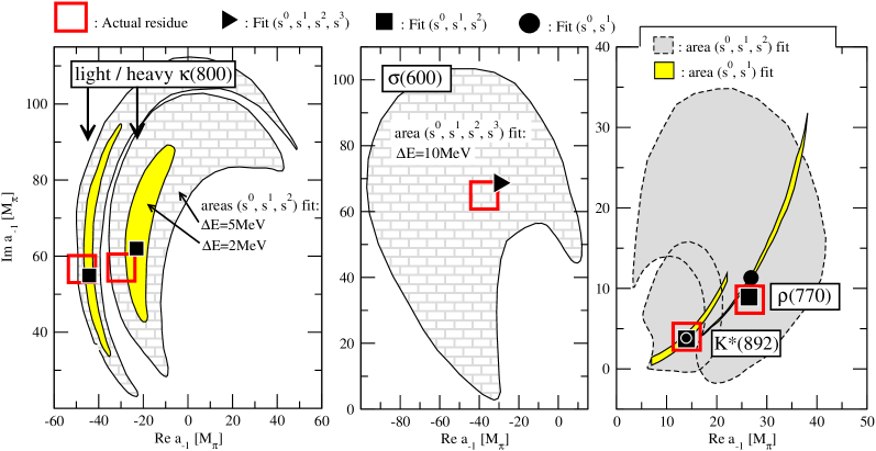
Figure 14: Residues of the resonances. The labeling of symbols and areas is precisely as in the figures of the respective resonances, 5,7, 10, 11, and 12. In the left panel, both cases of a heavy $\kappa(800)$ from section 3.2 and a light $\kappa(800)$ from section 3.3 are shown. The central panel shows the residues of the $\sigma(600)$ discussed in section 4.1, and in the right panel the residues of the $K^{*}(892)$ and $\rho(770)$ from section 4.2 are displayed.

To finish the resonance analysis, the residues of all analyzed resonances with their uncertainties are shown in figure 14. The displayed residues are defined as

$$T=\frac{a_{-1}}{E-z_{0}}+{\cal O}(E-z_{0})^{0}$$ (18)

where $z_{0}$ is the pole position in the upper half plane and $T$ is the transition within the lighter channel (on the second Riemann sheet), i.e. $\pi K\to~{}\pi K$ for the $\kappa(800)$ and the $K^{*}(892)$; $\pi\pi\to\pi\pi$ for the $\sigma(600)$ and the $\rho(770)$. Note that the residues for the poles at $z_{0}^{*}$ in the lower half plane are given as $a_{-1}(z_{0}^{*})=a_{-1}^{*}(z_{0})$. For the values of the actual residues, shown by the open (red) squares, the amplitude $T$ in eq. (18) is given by eq. (1), i.e. the solution that was used to generate the pseudo-data. For the fitted residues (central values, shown by filled (black) symbols, and areas), $T$ is given by eq. (10), using eq. (9) or (17) for the fit potential, depending on whether $S$- or $P$-wave states are analyzed.

The results shown in figure 14 suggest a similar interpretation as for the respective pole positions shown in figures 5,7, 10, 11, and 12: The residues of the broad $S$-wave resonances are much more difficult to determine than the residues of the $P$-wave states and require higher precision lattice data. For example, a $5$ MeV error for the lattice data of the $\kappa(800)$ barely fixes the sign of the real part of the residue. In contrast, with only a few lattice points from the lowest level and $10$ MeV error, the $(s^{0},\,s^{1})$ fits of the $K^{*}(892)$ and $\rho(770)$ resonances lead to a very narrow error band on the respective residues.

5 Conclusions

For the reconstruction of the $\kappa(800)$ resonance from lattice data, we have first performed a global fit to meson-meson partial wave data using the inverse amplitude method based on next-to-leading order terms of the chiral expansion. This allows to determine the low energy constants and to predict a pole position of $z_{0}=(815+i\,226)$ MeV for the $\kappa(800)$. This solution was used to generate pseudo-lattice data that were subsequently analyzed expanding a suitable fit potential systematically in powers of $s$. The key point is that the lowest-order chiral interaction serves as explicit input to the fit potential, considerably stabilizing the results. With a simple fit strategy the $\pi K$ phase and $\kappa(800)$ pole position together with the respective uncertainties could be determined in a model-independent way. To cover the possible pole positions of the $\kappa(800)$, we have also analyzed the case of a lighter $\kappa(800)$. As has been shown, a comprehensive resonance analysis requires rather high-precision lattice data. Still, using only one data point from the lowest level, one can at least make qualitative statements about the $\kappa(800)$. To put these results into context, we have also analyzed other channels using the same technique, showing that the $P$-wave resonances $K^{*}(892)$ and $\rho(770)$ are much easier to extract than the $S$-wave $\kappa(800)$ and $\sigma(600)$ resonances. The proposed analysis method allows not only to quantify the required precision of lattice data, but also helps to identify regions of the lattice spectrum that are particularly sensitive to resonance properties, which can contribute to minimize the practical effort in actual lattice simulations.

- (1) S. Dürr, Z. Fodor, J. Frison, C. Hoelbling, R. Hoffmann, S. D. Katz, S. Krieg, T. Kurth et al., Ab-Initio Determination of Light Hadron Masses, Science 322, 1224 (2008) [arXiv:0906.3599 [hep-lat]].
- (2) B. Blossier et al. [ European Twisted Mass Collaboration ], Light quark masses and pseudoscalar decay constants from N(f)=2 Lattice QCD with twisted mass fermions, JHEP 0804, 020 (2008) [arXiv:0709.4574 [hep-lat]].
- (3) H. -W. Lin et al. [ Hadron Spectrum Collaboration ], First results from 2+1 dynamical quark flavors on an anisotropic lattice: Light-hadron spectroscopy and setting the strange-quark mass, Phys. Rev. D79, 034502 (2009) [arXiv:0810.3588 [hep-lat]].
- (4) M. Göckeler et al. [ QCDSF Collaboration ], Extracting the rho resonance from lattice QCD simulations at small quark masses, PoS LATTICE2008, 136 (2008) [arXiv:0810.5337 [hep-lat]].
- (5) C. Gattringer, C. Hagen, C. B. Lang, M. Limmer, D. Mohler, A. Schäfer, Hadron Spectroscopy with Dynamical Chirally Improved Fermions, Phys. Rev. D79, 054501 (2009) [arXiv:0812.1681 [hep-lat]].
- (6) J. J. Dudek, R. G. Edwards, M. J. Peardon, D. G. Richards, C. E. Thomas, Toward the excited meson spectrum of dynamical QCD, Phys. Rev. D82, 034508 (2010) [arXiv:1004.4930 [hep-ph]].
- (7) R. Baron, P. Boucaud, J. Carbonell, A. Deuzeman, V. Drach, F. Farchioni, V. Gimenez, G. Herdoiza et al., Light hadrons from lattice QCD with light (u,d), strange and charm dynamical quarks, JHEP 1006, 111 (2010) [arXiv:1004.5284 [hep-lat]].
- (8) G. P. Engel et al. [ BGR [Bern-Graz-Regensburg] Collaboration ], Meson and baryon spectrum for QCD with two light dynamical quarks, Phys. Rev. D82, 034505 (2010) [arXiv:1005.1748 [hep-lat]].
- (9) X. Feng, K. Jansen, D. B. Renner, Resonance Parameters of the rho-Meson from Lattice QCD, Phys. Rev. D83 , 094505 (2011) [arXiv:1011.5288 [hep-lat]].
- (10) J. J. Dudek, R. G. Edwards, M. J. Peardon, D. G. Richards, C. E. Thomas, The phase-shift of isospin-2 scattering from lattice QCD, Phys. Rev. D83, 071504 (2011) [arXiv:1011.6352 [hep-ph]].
- (11) J. J. Dudek, R. G. Edwards, B. Joo, M. J. Peardon, D. G. Richards, C. E. Thomas, Isoscalar meson spectroscopy from lattice QCD, Phys. Rev. D83, 111502 (2011) [arXiv:1102.4299 [hep-lat]].
- (12) C. Morningstar, J. Bulava, J. Foley, K. J. Juge, D. Lenkner, M. Peardon, C. H. Wong, Improved stochastic estimation of quark propagation with Laplacian Heaviside smearing in lattice QCD, Phys. Rev. D83, 114505 (2011) [arXiv:1104.3870 [hep-lat]].
- (13) S. R. Beane et al. [ NPLQCD Collaboration ], The I=2 S-wave Scattering Phase Shift from Lattice QCD, [arXiv:1107.5023 [hep-lat]].
- (14) C. Morningstar, J. Bulava, J. Foley, Y. -C. Jhang, K. Juge, D. Lenkner, C. H. Wong, Excited-State Hadron Masses from Lattice QCD, [arXiv:1109.0308 [hep-lat]].
- (15) C. B. Lang, D. Mohler, S. Prelovsek, M. Vidmar, Coupled channel analysis of the rho meson decay in lattice QCD, Phys. Rev. D84, 054503 (2011) [arXiv:1105.5636 [hep-lat]].
- (16) B. J. Menadue, W. Kamleh, D. B. Leinweber, M. S. Mahbub, Isolating the in Lattice QCD, [arXiv:1109.6716 [hep-lat]].
- (17) Z. Fu, The preliminary lattice QCD calculation of meson decay width, [arXiv:1110.5975 [hep-lat]].
- (18) V. Bernard, U.-G. Meißner, A. Rusetsky, The Delta-resonance in a finite volume, Nucl. Phys. B788, 1 (2008) [arXiv:hep-lat/0702012].
- (19) M. Lüscher, Volume Dependence of the Energy Spectrum in Massive Quantum Field Theories. 2. Scattering States, Commun. Math. Phys. 105, 153 (1986).
- (20) M. Lüscher, Two particle states on a torus and their relation to the scattering matrix, Nucl. Phys. B354, 531 (1991).
- (21) M. Lüscher, Signatures of unstable particles in finite volume, Nucl. Phys. B364, 237 (1991).
- (22) J. A. Oller, E. Oset, J. R. Peláez, Meson meson interaction in a nonperturbative chiral approach, Phys. Rev. D59, 074001 (1999); [Erratum-ibid. D 60, 099906 (1999)]; [Erratum-ibid. D 75, 099903 (2007)]; [arXiv:hep-ph/9804209].
- (23) J. Gasser, H. Leutwyler, Chiral Perturbation Theory to One Loop, Annals Phys. 158, 142 (1984).
- (24) J. Gasser, H. Leutwyler, Chiral Perturbation Theory: Expansions in the Mass of the Strange Quark, Nucl. Phys. B250, 465 (1985).
- (25) V. Bernard, N. Kaiser, U.-G. Meißner, Threshold parameters of scattering in QCD, Phys. Rev. D43, 2757 (1991).
- (26) V. Bernard, N. Kaiser, U.-G. Meißner, scattering in chiral perturbation theory to one loop, Nucl. Phys. B357, 129 (1991).
- (27) V. Bernard, N. Kaiser, U.-G. Meißner, Chiral perturbation theory in the presence of resonances: Application to and scattering, Nucl. Phys. B364, 283 (1991).
- (28) J. A. Oller, E. Oset, Chiral symmetry amplitudes in the wave isoscalar and isovector channels and the , , scalar mesons, Nucl. Phys. A620, 438 (1997) [arXiv:hep-ph/9702314].
- (29) J. A. Oller, E. Oset, N/D description of two meson amplitudes and chiral symmetry, Phys. Rev. D60 , 074023 (1999) [arXiv:hep-ph/9809337].
- (30) M. Jamin, J. A. Oller, A. Pich, S wave scattering in chiral perturbation theory with resonances, Nucl. Phys. B587, 331 (2000) [arXiv:hep-ph/0006045].
- (31) M. Albaladejo, J. A. Oller, Identification of a Scalar Glueball, Phys. Rev. Lett. 101, 252002 (2008) [arXiv:0801.4929 [hep-ph]].
- (32) Z. -H. Guo, J. A. Oller, Resonances from meson-meson scattering in U(3) CHPT, Phys. Rev. D84, 034005 (2011) [arXiv:1104.2849 [hep-ph]].
- (33) G. Janssen, B. C. Pearce, K. Holinde and J. Speth, On the structure of the scalar mesons and , Phys. Rev. D 52, 2690 (1995) [arXiv:nucl-th/9411021].
- (34) O. Krehl, R. Rapp and J. Speth, Meson meson scattering: thresholds and mixing, Phys. Lett. B 390, 23 (1997) [arXiv:nucl-th/9609013].
- (35) A. Dobado, J. R. Peláez, A Global fit of and elastic scattering in ChPT with dispersion relations, Phys. Rev. D47, 4883 (1993) [hep-ph/9301276].
- (36) J. A. Oller, E. Oset, J. R. Peláez, Nonperturbative approach to effective chiral Lagrangians and meson interactions, Phys. Rev. Lett. 80, 3452 (1998) [arXiv:hep-ph/9803242].
- (37) J. Nieves, M. Pavón Valderrama, E. Ruiz Arriola, The Inverse amplitude method in scattering in chiral perturbation theory to two loops, Phys. Rev. D65, 036002 (2002) [hep-ph/0109077].
- (38) A. Gómez Nicola, J. R. Peláez, Meson meson scattering within one loop chiral perturbation theory and its unitarization, Phys. Rev. D65, 054009 (2002) [arXiv:hep-ph/0109056].
- (39) C. Hanhart, J. R. Peláez, G. Rios, Quark mass dependence of the and from dispersion relations and Chiral Perturbation Theory, Phys. Rev. Lett. 100, 152001 (2008) [arXiv:0801.2871 [hep-ph]].
- (40) J. Nebreda, J. R. Peláez., Strange and non-strange quark mass dependence of elastic light resonances from SU(3) Unitarized Chiral Perturbation Theory to one loop, Phys. Rev. D81, 054035 (2010) [arXiv:1001.5237 [hep-ph]].
- (41) J. Nebreda, J. R. Peláez, G. Rios, Mass dependence of pion-pion phase shifts within standard and unitarized ChPT versus Lattice results, [arXiv:1108.5980 [hep-ph]].
- (42) B. Ananthanarayan, G. Colangelo, J. Gasser, H. Leutwyler, Roy equation analysis of scattering, Phys. Rept. 353, 207 (2001) [arXiv:hep-ph/0005297 [hep-ph]].
- (43) I. Caprini, G. Colangelo, J. Gasser, H. Leutwyler, On the precision of the theoretical predictions for scattering, Phys. Rev. D68, 074006 (2003) [arXiv:hep-ph/0306122].
- (44) P. Büttiker, S. Descotes-Genon, B. Moussallam, A new analysis of scattering from Roy and Steiner type equations, Eur. Phys. J. C33, 409 (2004) [arXiv:hep-ph/0310283].
- (45) S. Descotes-Genon, B. Moussallam, The (800) scalar resonance from Roy-Steiner representations of scattering, Eur. Phys. J. C48, 553 (2006) [arXiv:hep-ph/0607133].
- (46) S. Descotes-Genon, Low-energy and scatterings revisited in three-flavour resummed chiral perturbation theory, Eur. Phys. J. C52, 141-158 (2007) [arXiv:hep-ph/0703154].
- (47) M. Hoferichter, D. R. Phillips, C. Schat, Roy-Steiner equations for , [arXiv:1108.4776 [hep-ph]].
- (48) V. Bernard, M. Lage, U.-G. Meißner, A. Rusetsky, Resonance properties from the finite-volume energy spectrum, JHEP 0808, 024 (2008) [arXiv:0806.4495 [hep-lat]].
- (49) V. Bernard, D. Hoja, U.-G. Meißner, A. Rusetsky, The Mass of the Delta resonance in a finite volume: fourth-order calculation, JHEP 0906, 061 (2009) [arXiv:0902.2346 [hep-lat]].
- (50) M. Lage, U.-G. Meißner, A. Rusetsky, A Method to measure the antikaon-nucleon scattering length in lattice QCD, Phys. Lett. B681, 439 (2009) [arXiv:0905.0069 [hep-lat]].
- (51) D. Hoja, U.-G. Meißner, A. Rusetsky, Resonances in an external field: The 1+1 dimensional case, JHEP 1004, 050 (2010). [arXiv:1001.1641 [hep-lat]].
- (52) V. Bernard, S. Descotes-Genon, G. Toucas, Chiral dynamics with strange quarks in the light of recent lattice simulations, JHEP 1101, 107 (2011) [arXiv:1009.5066 [hep-ph]].
- (53) V. Bernard, M. Lage, U.-G. Meißner, A. Rusetsky, Scalar mesons in a finite volume, JHEP 1101, 019 (2011) [arXiv:1010.6018 [hep-lat]].
- (54) M. Döring, U.-G. Meißner, E. Oset, A. Rusetsky, Unitarized Chiral Perturbation Theory in a finite volume: Scalar meson sector, [arXiv:1107.3988 [hep-lat]], accepted for publication in Eur. Phys. J. A.
- (55) A. M. Torres, L. R. Dai, C. Koren, D. Jido, E. Oset, The , interaction in finite volume and the resonance, [arXiv:1109.0396 [hep-lat]].
- (56) T. Luu, M. J. Savage, Extracting Scattering Phase-Shifts in Higher Partial-Waves from Lattice QCD Calculations, Phys. Rev. D83, 114508 (2011) [arXiv:1101.3347 [hep-lat]].
- (57) M. Döring, C. Hanhart, F. Huang, S. Krewald, U.-G. Meißner, D. Rönchen, The reaction in a unitary coupled-channels model, Nucl. Phys. A851, 58 (2011) [arXiv:1009.3781 [nucl-th]].
- (58) M. Döring, J. Haidenbauer, U.-G. Meißner, A. Rusetsky, Dynamical coupled-channel approaches on a momentum lattice, [arXiv:1108.0676 [hep-lat]].
- (59) K. Nakamura et al. [ Particle Data Group Collaboration ], J. Phys. G G37 , 075021 (2010).
- (60) D. Black, A. H. Fariborz, F. Sannino, J. Schechter, Evidence for a scalar resonance in scattering, Phys. Rev. D58, 054012 (1998) [arXiv:hep-ph/9804273].
- (61) E. M. Aitala et al. [ E791 Collaboration ], Dalitz plot analysis of the decay and indication of a low-mass scalar resonance, Phys. Rev. Lett. 89, 121801 (2002) [arXiv:hep-ex/0204018].
- (62) M. Ablikim et al. [ BES Collaboration ], The sigma pole in , Phys. Lett. B598, 149 (2004) [arXiv:hep-ex/0406038].
- (63) H. Q. Zheng, Z. Y. Zhou, G. Y. Qin, Z. Xiao, J. J. Wang, N. Wu, The kappa resonance in s wave scatterings, Nucl. Phys. A733, 235 (2004) [arXiv:hep-ph/0310293].
- (64) D. V. Bugg, The Kappa in E791 data for , Phys. Lett. B632, 471 (2006) [arXiv:hep-ex/0510019].
- (65) V. Bernard, E. Passemar, Matching chiral perturbation theory and the dispersive representation of the scalar form-factor, Phys. Lett. B661, 95 (2008) [arXiv:0711.3450 [hep-ph]].
- (66) K. Kampf, B. Moussallam, Chiral expansions of the lifetime, Phys. Rev. D79, 076005 (2009) [arXiv:0901.4688 [hep-ph]].
- (67) C. D. Froggatt, J. L. Petersen, Phase Shift Analysis of Scattering Between 1.0-GeV and 1.8-GeV Based on Fixed Momentum Transfer Analyticity, Nucl. Phys. B129, 89 (1977).
- (68) J. R. Batley et al. [ NA48/2 Collaboration ], New high statistics measurement of K(e4) decay form factors and scattering phase shifts, Eur. Phys. J. C54, 411 (2008).
- (69) D. Aston, N. Awaji, T. Bienz, F. Bird, J. D’Amore, W. M. Dunwoodie, R. Endorf, K. Fujii et al., A Study of K- pi+ Scattering in the Reaction at 11-GeV/c, Nucl. Phys. B296, 493 (1988).
- (70) D. Linglin, B. Chaurand, B. Drevillon, G. Labrosse, R. Lestienne, R. A. Salmeron, R. J. Miller, K. Paler et al., elastic scattering cross-section measured in 14.3 Gev/c interactions, Nucl. Phys. B57, 64 (1973).
- (71) P. Estabrooks, R. K. Carnegie, A. D. Martin, W. M. Dunwoodie, T. A. Lasinski, D. W. G. S. Leith, Study of Scattering Using the Reactions and at 13-GeV/c, Nucl. Phys. B133, 490 (1978).
- (72) L. Rosselet, P. Extermann, J. Fischer, O. Guisan, R. Mermod, R. Sachot, A. M. Diamant-Berger, P. Bloch et al., Experimental Study of 30,000 K(e4) Decays, Phys. Rev. D15, 574 (1977).
- (73) A. Schenk, Absorption and dispersion of pions at finite temperature, Nucl. Phys. B363, 97 (1991).
- (74) R. Mercer, P. Antich, A. Callahan, C. Y. Chien, B. Cox, R. Carson, D. Denegri, L. Ettlinger et al., scattering phase shifts determined from the reactions and , Nucl. Phys. 32B, 381 (1971).
- (75) P. Estabrooks, A. D. Martin, Phase Shift Analysis Below the Threshold, Nucl. Phys. B79, 301 (1974).
- (76) S. J. Lindenbaum, R. S. Longacre, Coupled channel analysis of J(PC) = 0++ and 2++ isoscalar mesons with masses below 2-GeV, Phys. Lett. B274, 492 (1992).
- (77) A. D. Martin, E. N. Ozmutlu, Analyses of production and scalar mesons, Nucl. Phys. B158, 520 (1979).
- (78) D. H. Cohen, D. S. Ayres, R. Diebold, S. L. Kramer, A. J. Pawlicki, A. B. Wicklund, Amplitude Analysis of the System Produced in the Reactions and at 6-GeV/c, Phys. Rev. D22, 2595 (1980).
- (79) A. Etkin, K. J. Foley, R. S. Longacre, W. A. Love, T. W. Morris, S. Ozaki, E. D. Platner, V. A. Polychronakos et al., Amplitude Analysis of the System Produced in the Reaction at 23-GeV/c, Phys. Rev. D25, 1786 (1982).
- (80) T. A. Armstrong et al. [WA76 and Athens-Bari-Birmingham-CERN-College de France Collaborations], Study of the system centrally produced in the reaction at 300-GeV/c, Z. Phys. C52, 389 (1991).
- (81) M. Döring, C. Hanhart, F. Huang, S. Krewald, U.-G. Meißner, Analytic properties of the scattering amplitude and resonances parameters in a meson exchange model, Nucl. Phys. A829, 170 (2009) [arXiv:0903.4337 [nucl-th]].
- (82) S. König, D. Lee, H.-W. Hammer, Volume Dependence of Bound States with Angular Momentum, Phys. Rev. Lett. 107, 112001 (2011) [arXiv:1103.4468 [hep-lat]].
- (83) S. König, D. Lee, H.-W. Hammer, Non-relativistic bound states in a finite volume, [arXiv:1109.4577 [hep-lat]].
- (84) S. R. Beane, P. F. Bedaque, A. Parreño, M. J. Savage, Two nucleons on a lattice, Phys. Lett. B585, 106 (2004) [arXiv:hep-lat/0312004].