next-nearest-neighbor tight-binding model of plasmons in graphene

Abstract

In this paper we investigate the influence of the next-nearest-neighbor coupling of tight-binding model of graphene on the spectrum of plasmon excitations. The nearest-neighbor tight-binding model was previously used to calculate plasmon spectrum in the next paper ziegler . We expand the previous results of the paper by the next-nearest-neighbor tight-binding model. Both methods are based on the numerical calculation of the dielectric function of graphene and loss function. Here we compare plasmon spectrum of the next-nearest and nearest-neighbor tight-binding models and find differences between plasmon dispersion of two models.

I 1 introduction

Graphene, a single layer of carbon atoms arranged as a honeycomb lattice, is a semimetal with remarkable physical properties kastro ; abergel . This is due to the band structure of the material which consists of two bands touching each other at two nodes. The electronic spectrum around these two nodes is linear and can be approximated by Dirac cones. However, calculations of many physical properties demand the knowledge of the full electron dispersion in the entire Brillouin zone, not only in the vicinity of the nodes. This statement becomes particularly relevant when we take into account the fact that graphene can be gated or doped, such that the Fermi energy can be freely tuned.

One of the main open issues in the physics of graphene is the role played by electron-electron interaction. In doped graphene long range Coulomb interaction leads to a gapless plasmon mode which can be described theoretically within the random phase approximation (RPA). Although this is a standard problem in semiconductor physics, it was studied initially in the case of graphene only in the Dirac approximation around the nodes wunsch ; hwang ; polini . The linear approximation leads to a frequency of the plasmon that is proportional to the square root of the wavevector.

Later the plasmon dispersion law was also calculated for the more realistic band structure, obtained in the framework of the tight-binding model with nearest-neighbor hopping ziegler ; katsnelson . This model is characterized by two symmetric bands, which implies a chiral symmetry. The latter connects the eigenstates of energy $-E$ directly with eigenstates of energy $E$ by a linear transformation. This symmetry, which also realizes a particle-hole symmetry, is broken by a next-nearest-neighbor hopping term. Usually, physically properties change qualitatively under symmetry breaking. Here we would like to study the effect of particle-hole symmetry breaking due to next-nearest-neighbor hopping on the plasmon dispersion. For this purpose we extend the nearest-neighbor hopping approximation used in ziegler by taking into account the next-nearest-neighbor hopping.

We consider an electron gas which is subject to an electromagnetic potential $V_{i}(\textbf{q},\omega)$. The response of the electron gas is to create a screening potential $V_{s}(\textbf{q},\omega)$ which is caused by the rearrangement of the electrons due to the external potential. Therefore, the total potential, acting on the electrons, isMahan

$$V(\textbf{q},\omega)=V_{i}(\textbf{q},\omega)+V_{s}(\textbf{q},\omega).$$ (1)

$V_{s}$ can be evaluated self-consistently Ehrenreich and is expressed via the dielectric function $\epsilon(\textbf{q},\omega)$. Then the total potential reads Mahan

$$V(\textbf{q},\omega)=\frac{1}{\epsilon(\textbf{q},\omega)}V_{i}(\textbf{q},\omega).$$ (2)

II 2 Nearest and next-nearest hopping model

The tight-binding Hamiltonian for electrons in graphene with both nearest- and next-nearest-neighbor hopping has the formkastro (we use units such that $\hbar=1$)

$$H= -t\sum_{<i,j>,\sigma}(a_{\sigma,i}^{\dagger}b_{\sigma,j}+H.c.)$$

$$-t^{\prime}\sum_{<<i,j>>,\sigma}(a_{\sigma,i}^{\dagger}a_{\sigma,j}+b_{\sigma,i}^{\dagger}b_{\sigma,j}+H.c.)$$ (3)

where $a_{\sigma,i}(a_{\sigma,i}^{\dagger})$ annihilates (creates) an electron with spin $\sigma(\sigma=\uparrow,\downarrow)$ on site $\textbf{R}_{i}$ on sublattice A (an equivalent definition is used for sublattice B), $t\approx 2.8$ eV is the nearest-neighbor hopping energy (hopping between different sublattices), and $t^{\prime}$ is the next nearest-neighbor hopping integral (hopping in the same sublattice). The value of $t^{\prime}$ is not well known but ab initio calculations find $0.02t\leq t^{\prime}\leq 0.2t$ depending on the tight-binding parametrization kastro .

The matrix representation of the Hamiltonian is

$$H=\begin{pmatrix}h_{0}&h_{1}-ih_{2}\\ h_{1}+ih_{2}&h_{0}\end{pmatrix}.$$ (4)

The non-diagonal terms in the Hamiltonian correspond to the nearest-neighbor hoppingziegler :

$$h_{1}=-t\sum_{j=1}^{3}\cos(\textbf{b}_{j}\textbf{k}),\quad h_{2}=-t\sum_{j=1}^{3}\sin(\textbf{b}_{j}\textbf{k}),$$ (5)

where $\textbf{b}_{1,2,3}$ are the nearest-neighbor vectors on the honeycomb lattice: $\textbf{b}_{1}=d(1/2,\sqrt{3}/2),\textbf{b}_{2}=d(1/2,-\sqrt{3}/2)\textbf{b}_{3}=d(-1,0)$ and $d$ is the lattice constant ($\approx$ 1.42 Å). The diagonal terms correspond to next-nearest-neighbor hopping:

$$h_{0}=-t^{\prime}\sum_{j=1}^{6}\cos(\textbf{a}_{j}\textbf{k}),$$ (6)

where $\textbf{a}_{1}=d(3/2,\sqrt{3}/2),\textbf{a}_{2}=d(-3/2,-\sqrt{3}/2),\textbf{a}_{3}=d(3/2,-\sqrt{3}/2),\textbf{a}_{4}=d(-3/2,\sqrt{3}/2),\textbf{a}_{5}=d(0,-\sqrt{3}),\textbf{a}_{6}=d(0,\sqrt{3})$.

The energy bands derived from this Hamiltonian have the formkastro

$$E_{\pm}({\bf k}) =\pm t\sqrt{3+f(\textbf{k})}-t^{\prime}f(\textbf{k}),$$

$$f(\textbf{k}) =2\cos(\sqrt{3}k_{y}a)+4\cos(\frac{\sqrt{3}}{2}k_{y}a)\cos(\frac{3}{2}k_{y}a)$$ (7)

where the plus sign applies to the upper ($\pi$ or conduction) and the minus sign the lower ($\pi*$ or valence) band. It should be noticed that the presence of $t^{\prime}$ shifts the position of the Dirac point in energy and it breaks electron-hole symmetry. In both cases, nearest-neighbor and next nearest-neighbor hopping, the electronic dispersion is an even functionziegler

$$E_{\textbf{k},l}=E_{-\textbf{k},l}\ .$$ (8)

The dispersion law for next nearest-neighbor hopping is presented on Fig. 1,

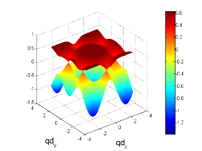
Figure 1: Energy dispersion of graphene with $t^{\prime}=0.2t$. The figure shows a broken particle–hole symmetry. The Dirac nodes are shifted up by $3t^{\prime}$. The energy is measured in the units of the electronic bandwith $\Delta=3t$.

and the eigenvectors of the Hamiltonian read

$$\frac{1}{\sqrt{2}}\begin{pmatrix}\frac{h_{1}-ih_{2}}{\sqrt{h_{1}^{2}+h_{2}^{2}}}\\ 1\end{pmatrix},\frac{1}{\sqrt{2}}\begin{pmatrix}\frac{h_{1}-ih_{2}}{\sqrt{h_{1}^{2}+h_{2}^{2}}}\\ -1\end{pmatrix}$$ (9)

where the first eigenvector is for the upper band and the second eigenvector for the lower band.

The Hamiltonian $H$ in Eq. (4) has a chiral symmetry for $h_{0}=0$:

$$e^{\alpha\sigma_{3}}He^{\alpha\sigma_{3}}=H,\ \ \ \sigma_{3}=\begin{pmatrix}1&0\\ 0&-1\end{pmatrix}\ ,$$ (10)

which connects eigenstates of energy $-E$ with eigenstates of energy $E$ by

$$\Psi_{-E}=\sigma_{3}\Psi_{E}\ .$$ (11)

This is not the case after we have broken the chiral symmetry by the next-nearest-neighbor hopping term $h_{0}$.

III 3 Dielectric Function

The longitudinal dielectric function in calculated in RPADressel ; Ehrenreich :

$$\epsilon(\textbf{q},\omega)=1-\frac{2\pi e^{2}}{q\kappa}\chi(\textbf{q},\omega)$$ (12)

where $\kappa$ is a dielectric constant and $\chi$ is a polarizability. For polarizability we used the Lindhard formula Dressel , which in our case after some straightforward calculations can be reduced to the expression

$$\chi(\textbf{q},\omega)=\chi_{1}(\textbf{q},\omega)+\chi_{2}(\textbf{q},\omega)$$ (13)

with the intraband contribution

$$\chi_{1}(\textbf{q},\omega)=\lim_{\delta\to 0}\sum_{s,t=\pm 1}\int\limits_{BZ}\frac{1}{4}|\kappa_{\textbf{k}}^{*}\kappa_{\textbf{k+q}}+1|^{2}$$ (14)

$$\times\frac{f(sE_{\textbf{k}}^{(1)}+E_{\textbf{k}}^{(2)})}{s\left(E_{\textbf{k}}^{(1)}-E_{\textbf{k + q}}^{(1)}\right)+E_{\textbf{k}}^{(2)}-E_{\textbf{k + q}}^{(2)}+t(\omega-i\delta)}d^{2}k,$$

and the interband contribution

$$\chi_{2}(\textbf{q},\omega)=\lim_{\delta\to 0}\sum_{s,t=\pm 1}\int\limits_{BZ}\frac{1}{4}|\kappa_{\textbf{k}}^{*}\kappa_{\textbf{k+q}}-1|^{2}$$ (15)

$$\times\frac{f(sE_{\textbf{k}}^{(1)}+E_{\textbf{k}}^{(2)})}{s\left(E_{\textbf{k}}^{(1)}+E_{\textbf{k + q}}^{(1)}\right)+E_{\textbf{k}}^{(2)}-E_{\textbf{k + q}}^{(2)}+t(\omega-i\delta)}d^{2}k,$$

where

$$\kappa_{{\bf k}}=(h_{1}-ih_{2})/E_{{\bf k}},$$ (16)

$$h_{1}=-t\left[\cos(k_{x}d)\cos(\sqrt{3}k_{y}d)+\cos(k_{s}d)\right],$$

$$h_{2}=-t\left[\sin(k_{x}d)\cos(\sqrt{3}k_{y}d)+\sin(k_{s}d)\right];$$

$f(E)=1/(e^{\beta(E-\mu)}+1)$ is the Fermi-Dirac distribution function, $\beta=1/k_{B}T$, $\mu$ is a chemical potential. The energies are defined as

$$E_{\textbf{k},l}=E_{\textbf{k},l}^{(1)}+E_{\textbf{k},l}^{(2)},$$ (17)

$$E_{\textbf{k},l}^{(1)}=(-1)^{l}\sqrt{h_{1}^{2}+h_{2}^{2}}=\pm t\sqrt{3+f(\textbf{k})},$$

$$E_{\textbf{k},l}^{(2)}=-t^{\prime}f(\textbf{k})$$

If we take $E_{\textbf{k}}^{(2)}=E_{\textbf{k+q}}^{(2)}=0$ the integral yields the same polarizability formula as that found in the nearest-neighbor model’s polarizability ziegler ; katsnelson .

IV 4 plasmons in graphene

In a first approximation, we can consider plasmons as collective excitations of electrons, where the dielectric function vanishesMahan :

$$\epsilon(\textbf{q},\omega)=0.$$ (18)

In general, however, the dielectric function is complex due to poles in the integrals (14), (15). This implies that (18) has no solution, unless we only request that the real part of the dielectric function vanishes:

$$Re[\epsilon(\textbf{q},\omega)]=0,$$ (19)

assuming a real function $\omega({\bf q})$ as the plasmon dispersion. For a numerical evaluation of the integrals it is more convenient to consider the loss functionpolini ; Mahan ; Dressel

$$Im\Bigg{(}\frac{1}{\epsilon(\textbf{q},\omega)}\Bigg{)}=\frac{-Im[\epsilon(\textbf{q},\omega)]}{\{Re[\epsilon(\textbf{q},\omega)]\}^{2}+\{Im[\epsilon(\textbf{q},\omega)]\}^{2}}$$

whose broadened peak indicates the plasmon. Here a complex solution $\omega({\bf q})$ gives both the dispersion from the real part and the decay of the plasmons from the imaginary part.

In the present paper the polarizability of graphene $\chi$ is evaluated numerically and the corresponding dielectric function is obtained from Eq. (12) for different values of the real frequency $\omega$, the wave vector ${\bf q}$ and chemical potential (Fermi energy) $\mu$. Moreover, we assume $\kappa=4$. The chemical potential level $\mu$ is selected to be relative to Dirac points whose existence is not affected by a variation of the parameter $t^{\prime}$ but are shifted by $3t^{\prime}$ (ref. wallace ), as shown in Fig. [ 2].

Our results for plasmon dispersion law are shown in Figs. 3 and 4. For each figure we have selected two values for $t^{\prime}$, namely $t^{\prime}=0$ and $t^{\prime}=0.2t$. The original chemical potentials $\mu$ that appear in Figs. 3 and 4 are taken from the previous paper ziegler and are modified by the value $t^{\prime}=0.2t$.

The influence of next-nearest hopping parameter $t^{\prime}$ is insignificant for the plasmon dispersion law when the chemical potential is above Dirac point, as depicted in Figs. 3 and 4. The shape of the plasmon dispersion law in Fig. 3 does not change significantly by a variation of the parameter $t^{\prime}=0,0.2t$. On the other hand, the result is quite different when the chemical potential is below the Dirac point. Fig. 4 shows that for different values of hopping parameter $t^{\prime}$ and for a negative chemical potential the shape of dispersion law changes strongly and the dispersion curve is much sharper when the value of the hopping parameter is larger. In general, our calculations of the plasmon dispersion law show that there is almost no change of the plasmon dispersion with $t^{\prime}$ when chemical potential is above the Dirac point.

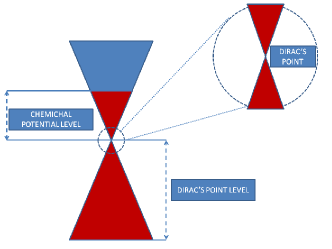
Figure 2: The scheme shows that chemical potential $\mu$ is taken relative to Dirac cone. Dirac point’s level is relative to case $t^{\prime}=0$ and the level equals to $3t^{\prime}$ .

V 5 conclusion

In conclusion we have investigated the 2D tight-binding hamiltonian model under the influence of the next nearest-neighbour coupling (constant) and we theoretically obtained analytic expression for improved graphene polarizability expression . Our work is extension to previous results obtained by ziegler , where only near-neighbor constant model is used. This work improves the previous results for graphene plasmon’s dispersion law.

The research of next-nearest hopping tight-binding model gave the possibility to investigate the plasmon’s dispersion law near Dirac point in the case of low values of chemical potential relative to Dirac point, by using analytical calculations and numerically to show that dispersion’s laws in two cases (near neighbor and next-nearest tight binding model) are almost the same as predicted theoretically.

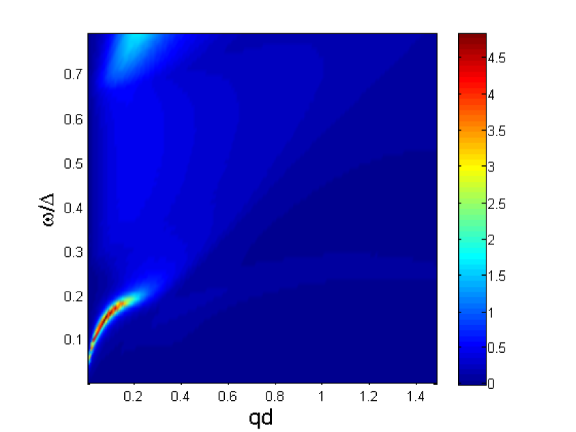
(a) Plasmon dispersion for $\mu=0.4t,t^{\prime}=0.0t$ and different values of $q_{y}$ component ($q_{x}=0$)

(b) Plasmon dispersion for $\mu=0.4t,t^{\prime}=0.2t$ and different values of $q_{y}$ component ($q_{x}=0$)

Figure 3: Plasmon dispersion for $\mu=0.4t$

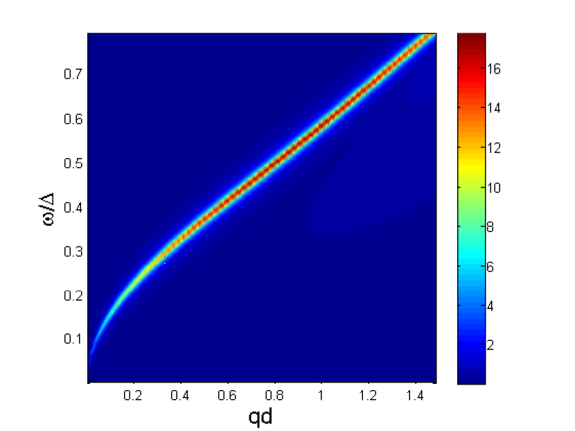
(a) Plasmon dispersion for $\mu=-2.7t,t^{\prime}=0.0t$ and different values of $q_{y}$ component ($q_{x}=0$)

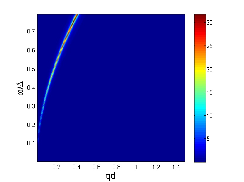
(b) Plasmon dispersion for $\mu=-2.7t,t^{\prime}=0.2t$ and different values of $q_{y}$ component ($q_{x}=0$)

Figure 4: Plasmon dispersion for $\mu=-2.7t$

References

- (1) A. Hill, S. A. Mikhailov, K. Ziegler, EPL 87, 27005 (2009).
- (2) A. H. Castro Neto, F. Guinea, N. M. R. Peres, K. S. Novoselov and A. K. Geim, Rev. Mod. Phys. 81, 109 (2009).
- (3) D.S.L. Abergel, V. Apalkov, J. Berashevich, K. Ziegler, T. Chakraborty, Adv. Phys. 59, 261 (2010).
- (4) B. Wunsch, T. Stauber, F. Sols and F. Guinea, New J. Phys. 8, 318 (2006).
- (5) E. H. Hwang and S. Das Sarma, Phys. Rev B 75, 205418 (2007).
- (6) M. Polini and R. Asgari and G. Borghi and Y. Barlas and T. Pereg-Barnea and A. H. MacDonald, Phys. Rev. B. 77, 081411(R) (2008).
- (7) S. Yuan, R. Roldan, M. I. Katsnelson, Phys. Rev. B 84, 035439 (2011).
- (8) G. Mahan, Many particle physics, Plenum Pr., New York, (1990).
- (9) H. Ehrenreich and M.H. Cohen, Phys. Rev. 115, 786 (1959).
- (10) M. Dressel,G. Gruner, Electrodynamics of Solids: Optical Properties of Electrons in Matter, Cambridge University Press, (2002).
- (11) P. R. Wallace, Phys. Rev. 71, 622 (1947).