Fluctuations in the number of intermediate mass fragments in small projectile like fragments.

Abstract

The origin of fluctuations in the average number of intermediate mass fragments seen in experiments in small projectile like fragments is discussed. We argue that these can be explained on the basis of a recently proposed model of projectile fragmentation.

This report is an outgrowth of a recent work Mallik2 where we introduced a model of projectile fragmentation in heavy ion collisions. The model has three ansatzs: at a given impact parameter a certain part of the projectile is sheared off forming a projectile like fragment (PLF) with charge number $Z_{s}$ and neutron number $N_{s}$. This is called abrasion. This hot PLF expands to about one-third the normal density and then breaks up into several composites at a given temperature $T$. This break up is according to a canonical thermodynamical model (CTM). The composites are hot and will decay by evaporation. For details, please see Mallik2 . The main contention of reference Mallik2 was that the temperature $T$ must be taken to be a function of the impact parameter $b$.

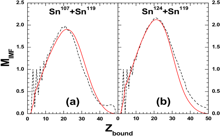
Figure 1: (Color Online) Mean multiplicity of intermediate-mass fragments $M_{IMF}$, as a function of $Z_{bound}$ for (a) ¹⁰⁷Sn on ¹¹⁹Sn and (b) ¹²⁴Sn on ¹¹⁹Sn reaction (red solid lines). Temperature is impact parameter ($b$) dependent and falls off linearly with b from $7.5$ MeV at $b$=0 to $3$ MeV at maximum value of $b$. The experimental results Ogul are shown by the black dashed lines.

Results of the following experiment done at the SIS heavy-ion synchrotron at GSI Darmstadt are published Ogul . In an event let us denote the number of intermediate mass fragments (IMF) (charge $z$ between 3 and 20) by $N_{IMF}$. In the same event denote by $Z_{bound}$=sum of all the charges in the PLF minus the charges of $z=1$ particles (proton, deuteron and triton). After many events one can plot $M_{IMF}$ $\it{vs}$ $Z_{bound}$ where $M_{IMF}$ is the average of $N_{IMF}$. The data and comparison with the theoretical calculation done in Mallik2 is shown in Fig. 1.

	$M_{IMF}$
$Z_{bound}$	$Sn^{107}$	$Sn^{124}$	$La^{124}$
3	1.000	1.000	1.000
4	0.140	0.000	0.178
5	1.000	1.000	1.000
6	0.430	0.565	0.620
7	1.062	1.078	1.092

Table 1: Experimentally measured $M_{IMF}$ at small $Z_{bound}$ values for $Sn^{107}$ on $Sn^{119}$, $Sn^{124}$ on $Sn^{119}$ and $La^{124}$ on $Sn^{119}$ reactions.

The overall feature of the figure is that the general shapes of the theoretical and experimental curves agree. The $b$ dependence of $T$ is crucial for this (as explained in Mallik2 ). However, there are significant fluctuations in the experimental values of $M_{IMF}$ for low values of $Z_{bound}$ whereas theory completely misses these fluctuations. In this note we explain (a)why these fluctuations arise, (b) how staying within the main ingredients of the theoretical model but using more realistic parameters we can reproduce the fluctuations and (c) why the calculation in Mallik2 missed the fluctuations seen in small PLF’s.

First we explain how the fluctuations arise. We have $Z_{bound}$=$Z_{s}$ minus the sum of charges of all $z$=1 particles (protons, deuterons and tritons). Also a particle is considered to be an IMF if its charge $z$ is between 3 and 20. Just these two conditions and some general knowledge of low-mass nuclei allow us to reach some interesting conclusions.

If $Z_{bound}$=3 it guarantees that we have a ${}^{A}_{3}$Li nucleus. Thus for $Z_{bound}$=3 $M_{IMF}$=1. If ${}^{A}_{3}$Li decays by a proton emission we are no longer in $Z_{bound}$=3 but degenerate into $Z_{bound}$=2. Also there is no IMF. If it decays by neutron emission to a particle stable state of a different isotope of Li, we still have $M_{IMF}$=1. There are several particle stable states of Li so $Z_{bound}=3$, $M_{IMF}$=1 is always satisfied.

Let us consider now $Z_{bound}$=4. For $Z_{bound}$=4 we can have a Be nucleus with $N_{IMF}$=1 but it can also decay into two He isotopes which still retains $Z_{bound}$=4 but with $N_{IMF}$=0. We therefore expect to have $Z_{bound}$=4 and $M_{IMF}=X$ where $X$ is less than 1. But unfortunately $X$ is not the same value for all Be nuclei. We will soon demonstrate how $X$ could be determined for each Be nucleus but the fact that $X$ varies from one isotope of Be to another isotope of Be makes the evaluation of $M_{IMF}$ in the case of $Z_{bound}$=4 a lengthy procedure.

If $Z_{bound}$=5 we have either one Boron nucleus or a Li nucleus plus a He nucleus. In both the cases $M_{IMF}$=1. If the Boron nucleus sheds a proton, the status drops to $Z_{bound}$=4 and we are back to the $Z_{bound}$=4 case. If the Boron nucleus sheds one or more neutrons to reach a particle stable state we maintain $Z_{bound}=5,M_{IMF}$=1. If Boron decays into a Li and He two things can happen. We reach a particle stable state of Li and we have $Z_{bound}=5$, $M_{IMF}$=1. If the Li sheds a proton we no longer have $Z_{bound}$=5. Thus so long as we have $Z_{bound}$=5 we have $M_{IMF}$=1.

We want to get back to the case of $Z_{bound}$=4. Now we need to bring in details of the model. Two modifications are made. To carry out CTM one needs to put in the partition function of each composite into which the hot abraded PLF can break into. In our previous calculation, except for nuclei upto ⁴He, we used the liquid-drop model for the ground state energy and the Fermi-gas model for excited states. For small PLF’s this is inaccurate and we put in experimental values of ground state and excited state energies. Usually all excited states upto 7.5 MeV are included. Next we consider the decays of hot composites resulting from CTM. Previously we used an evaporation code. We replace this by actual decay data whenever possible. In practical terms this means the following. A nucleus has many energy levels and a hot nucleus means that the probability of occupation of a state $i$ is proportional to $s_{i}exp(-exc(i)/T))$ where $s_{i}$ is the spin degeneracy and $exc(i)$ is the excitation energy. The decay of the state $i$ is taken from data table Ajzenberg1 ; Ajzenberg2 ; Tilley1 ; Tilley2 ; www1 where available or guessed from systematics. We take $T$ to be 7 MeV suggested by our past work Mallik2 .

It is useful to list first the deacy properties of hot Be nuclei. These are computed at $T$=7 MeV.

${}^{6}_{4}$Be: This decays into Ajzenberg1 ${}^{4}_{2}$He plus 2 protons so this counts as $Z_{bound}$=2 and $M_{IMF}$=0.

${}^{7}_{4}$Be: The lowest 2 states are particle stable. Population into any of these gives $Z_{bound}$=4 and one IMF. The probability of this occurring is 0.406. The other states decay into ${}^{4}_{2}$He plus ${}^{3}_{2}$He leading to $Z_{bound}$=4 and $N_{IMF}$=0. Thus for ${}^{7}_{4}$Be we have $Z_{bound}$=4 and $M_{IMF}$=0.406.

${}^{8}_{4}$Be: this occurs as resonances of two ${}^{4}_{2}$He so here $Z_{bound}$=4 and $M_{IMF}$=0.

${}^{9}_{4}$Be: Only the ground state is particle stable, the rest decay to neutron plus two alphas. The occupation probability in the ground state is 0.193. So here $Z_{bound}$=4 and $M_{IMF}$=0.193.

${}^{10}_{4}$Be: Here we have taken all the levels upto 6.26 MeV (summed occupation probability=0.604) to give $Z_{bound}$=4 and 1 IMF and rest of the levels upto 9.3 MeV to give $Z_{bound}$=4 and 0 IMF. Thus $Z_{bound}$=4 and $M_{IMF}$=0.604.

${}^{11}_{4}$Be: Here the lowest two levels have $Z_{bound}$=4 and $N_{IMF}$=1 and the probability of occupation 0.1567. The higher levels, with summed occupation probability 0.8433 go to ${}^{10}_{4}$Be+n. We have assigned them $Z_{bound}$=4 and $M_{IMF}$=0.604. Thus we take ${}^{11}_{4}$Be to give $Z_{bound}$=4 and $M_{IMF}$=0.666.

Let us now outline how we calculate $M_{IMF}$ for $Z_{bound}$=4 for collisions of ¹⁰⁷Sn, ¹²⁴Sn and ¹²⁴La on ¹¹⁹Sn. Although our discussion will be limited to $Z_{bound}$=4, the method can be extended to higher values of $Z_{bound}$ except that the complexity increases very rapidly. The method of obtaining the abrasion cross-section for a PLF with given $Z_{s},N_{s}$ is given in Mallik2 . For $Z_{bound}$=4 we need to consider $Z_{s}$=4 (most important) and higher. Once a PLF with given $Z_{s},N_{s}$ is formed it will expand to one-third the normal nuclear density and break up into hot composites. Just as we could characterize a hot Be nucleus by a $Z_{bound}$ and $M_{IMF}$ we can ascribe to each $Z_{s},N_{s}$ a probability of obtaining $Z_{bound}$=4 with an associated $M_{IMF}$. (An example below shows how this can be done.) Table II compiles these values (last two columns).

		Cross-section (mb)
$Z_{s}$	$N_{s}$	$Sn^{107}$	$Sn^{124}$	$La^{124}$	$P(Z_{bound}=4)$	$M_{IMF}$
4	3	0.6597	0.0	0.0	0.605	0.406
4	4	8.9445	0.5644	5.1102	0.583	0.043
4	5	10.5290	4.5058	8.3227	0.569	0.165
4	6	1.1099	8.8110	0.6300	0.486	0.448
4	7	0.0	3.7233	0.0	0.467	0.592
5	4	0.4406	0.0	0.0	0.6087	0.074
5	5	7.7417	0.0	4.5875	0.2842	0.125
5	6	12.8264	2.1752	11.4830	0.2304	0.194
5	7	1.5797	9.2460	2.5002	0.1926	0.336
5	8	0.0	8.5111	0.0	0.1782	0.498

Table 2: Abrasion cross-sections (in millibarns) for a given ($Z_{s}$, $N_{s}$) for $Sn^{107}$, $Sn^{124}$ and $La^{124}$ on $Sn^{119}$. $P(Z_{bound}=4)$ gives the probability of obtaining $Z_{bound}=4$ for a given $Z_{s}$, $N_{s}$ and $M_{IMF}$ is the corresponding average multiplicity of intermediate mass fragments.

Utilizing also the values of the abrasion cross-sections for $Z_{s},N_{s}$ for the three reactions (also given in the Table) we get the desired results. For $Z_{bound}$=4, $M_{IMF}$=0.145(0.14) for ¹⁰⁷Sn beam, 0.151(0.178) for ¹²⁴La beam and 0.38(0) for ¹²⁴Sn beam. The experimental values are enclosed by parenthesis. Except for ¹²⁴Sn beam our results approximately correspond to the experimental data. The value 0 for ¹²⁴Sn is a mystery. In any model we can think of the result should not be 0 or very different from the other two. In any case we have reproduced the fluctuation: $M_{IMF}$ drops from 1 at $Z_{bound}$=3 to much lower value at $Z_{bound}$=4 and back again to 1 at $Z_{bound}$=5. It is very long to do a quantitative estimate for $Z_{bound}$=6. This will arise from $Z_{s}$=6 and higher. A study of the CTM results of $Z_{s}=6,N_{s}=7$ shows the following. There is a significant probability of reaching a Carbon nucleus ($Z_{bound}$=6). This will produce a $M_{IMF}\approx$1. There is a comparable probability of obtaining $Z_{bound}$=6 with a ⁸Be nucleus (zero IMF) and another He nucleus and also a ⁹Be nucleus ($M_{IMF}$=0.193) and another He nucleus. The probability of reaching two Li nuclei post CTM is non-negligible but the chances of any one or both of them decaying by alpha or proton emission (thereby dropping below $Z_{bound}$=6) are quite high (0.88). A theoretical value for $M_{IMF}\approx$0.5 seems quite plausible. It is the fragility of $Be$ nuclei which produces the dip in $M_{IMF}$ for $Z_{bound}$=4 and is also responsible for the dip at $Z_{bound}$=6.

$A$	$Z$	$<n_{A,Z}>$	$A$	$Z$	$<n_{A,Z}>$
9	4	$4.7518\times 10^{-1}$	5	3	$8.0475\times 10^{-3}$
8	4	$8.8281\times 10^{-2}$	5	2	$1.2987\times 10^{-1}$
8	3	$3.8108\times 10^{-2}$	4	2	$1.3924\times 10^{-1}$
7	4	$5.8888\times 10^{-3}$	3	2	$2.4670\times 10^{-2}$
7	3	$1.0194\times 10^{-1}$	3	1	$1.0669\times 10^{-1}$
6	4	$1.1442\times 10^{-4}$	2	1	$1.5234\times 10^{-1}$
6	3	$1.0470\times 10^{-1}$	1	1	$7.4883\times 10^{-2}$
6	2	$2.1149\times 10^{-2}$	1	0	$1.8152\times 10^{-1}$

Table 3: Multiplicity of different fragments produced by CTM from the abraded nucleus $Z_{s}=4$, $N_{s}=5$ at $T=7.0$ MeV.

As promised, let us give an example how for a given $Z_{s},N_{s}$ the probability of occurrence of $Z_{bound}$=4 and the associated $M_{IMF}$ can be computed (last two columns of Table II). Consider $Z_{s}=4,N_{s}=5$. To start with, the average numbers of each composite resulting from the CTM break up of $Z_{s}=4,N_{s}=5$ system are listed in Table III. But in a simple case like this, this can also give, with little effort, the probability of a channel or the probability of a sum of channels. From the table, the average number of ${}^{9}_{4}$Be is $\approx$0.475. This is a channel where only ${}^{9}_{4}$Be and nothing else appears. Thus there is a probability of 0.475 of reaching $Z_{bound}$=4 and $M_{IMF}$=0.193. Next, looking at the table, the average number of ⁸Be is $\approx$0.088. This comes from a channel where there is one ⁸Be and one neutron. So we have a probability of 0.088 of reaching $Z_{bound}$=4 with $M_{IMF}$=0.0. Next from the table, the average number of ${}^{8}_{3}$Li is $\approx$0.038. This has to occur in combination with a proton. Clearly, this is channel with $Z_{bound}$=3, so this does not concern us presently. Next, from the table, the average number of ${}^{7}_{4}$Be is $\approx$0.006. This is a channel which has one ${}^{7}_{4}$Be and 2 neutrons. Thus we have a probability of 0.006 of reaching $Z_{bound}$=4 with $M_{IMF}$= 0.406. We have exhausted all the channels for reaching $Z_{bound}$=4. Summing up with appropriate weightage, from $Z_{s}=4,N_{s}=5$ the probability of reaching $Z_{bound}$=4 is 0.569 with $M_{IMF}$=0.165.

We can repeat similar arguments for other $Z_{s},N_{s}$ in Table II. The cases of $Z_{s}$=5 are more complicated.

We now try to answer why the calculation of Mallik2 failed to produce any fluctuation. There are many reasons (use of liquid-drop model and non-recognition of the fragility of Be nucleus etc.) but the most interesting reason is different.

The prescription we used for $M_{IMF}$ vs. $Z_{bound}$ is the following. At a given $b$, abrasion gives an integral $Z_{s}$ (and an integral $N_{s}$). This system expands, then dissociates by CTM and the hot composites which are the end results of the CTM, can evaporate light particles to give the final distribution. From this we obtained $M_{IMF}$ and we considered $Z_{bound}$ to be given by $Z_{s}-\sum_{i}n_{z=1}(i)$ where $n_{z=1}(i)$ stands for the average multiplicity of proton/deuteron/triton. This prescription does not match exactly the experimental procedure. Experimentally $Z_{bound}$ is obtained event by event and in every event $Z_{bound}$ is an integer (sum of all charges from PLF minus number of particles with $z$=1). From many events with the same $Z_{bound}$ one can obtain $M_{IMF}$. In our calculations although $Z_{s}$ is an integer $Z_{s}-\sum_{i}n_{z=1}(i)$ will usually be non-integer since the $n_{z=1}(i)$’s (average number of composite $i$) are.

Our calculation can map much better into a different experiment. In this experiment $Z_{s}$ is measured but $z$=1 particles are not subtracted. One then obtains $M_{IMF}$ for each $Z_{s}$. This problem is simpler: given a total number of particles, what is $M_{IMF}$? But in the reported experiment one asks a more exclusive question : when the particles are fractured in a certain way (a given number of particles with charge greater than 1) what is $M_{IMF}$? In our prescription we get a non-integral value for $Z_{bound}$ and what we are obtaining is an average of $M_{IMF}$ done over $M_{IMF}$ belonging to different but neighbouring values of integral $Z_{bound}$. This would be quite wrong if values of $M_{IMF}$ belonging to neighbouring $Z_{bound}$’s differ strongly (as it happens for very small systems) but for large systems the difference would be small and our prescription is adequate for an estimate.
This work was supported in part by Natural Sciences and Engineering Research Council of Canada. The authors are thankful to Prof. Wolfgang Trautmann for access to experimental data. S. Mallik is thankful for a very productive and enjoyable stay at McGill University for this work. S. Das Gupta wants to thank Prof. Jean Barrette for discussions.

References

- (1) S. Mallik, G. Chaudhuri and S. Das Gupta, arxiv:nucl-th/1108.4351v1, To be published in Phys. Rev C
- (2) R. Ogul et al., Phys. Rev C 83, 024608(2011).
- (3) F.Ajzenberg-Selove and T. Lauritsen, Nucl. Phys. A 227, 1 (1974).
- (4) F.Ajzenberg-Selove and T. Lauritsen, Nucl. Phys. A 248, 1 (1975).
- (5) D.R.Tilley et al., Nucl. Phys. A 708, 3 (2002).
- (6) D.R.Tilley et al., Nucl. Phys. A 745, 155 (2004).
- (7) http://www.nndc.bnl.gov/ensdf/index.jsp