Kinematic formation of the pseudogap spectral properties in a spatially homogeneous strongly correlated electron system

Abstract

It is shown that the kinematic interaction caused by the quasi-Fermi character of commutation relations for operators of the atomic representation can induce pseudogap behavior of the spectral characteristics of an ensemble of Hubbard fermions. Mathematically, the presence of the kinematic interaction manifests itself in modification of the faithful representation of a single-particle Green’s function of Hubbard fermions $D(\textbf{k},i\omega_{n})$, which involves, apart from self-energy operator $\Sigma_{L}(\textbf{k},i\omega_{n})$, strength operator $P(\textbf{k},i\omega_{n})$. It is important that the strength operator enters both the numerator and the denominator of the exact expression for $D(\textbf{k},i\omega_{n})$. The kinematic interaction, therefore, not only renormalizes the spectrum of elementary excitations but significantly affects their spectral weight. It results in strong modulation of spectral intensity $A(\textbf{k},\omega)$ occurring on a Fermi contour. Calculations of the spectral properties for the $t-J$ model in the one-loop approximation yield good quantitative agreement with the ARPES data obtained on cuprate superconductors.

PACS numbers

71.10.Fd, 71.18.+y, 71.27.+a, 74.40.-n, 74.72.Kf

I Introduction

The normal phase of cuprate superconductors is characterized by a number of intriguing properties that cannot be described within the traditional Fermi liquid theory. These are, first of all, the pseudogap behavior in an undoped region Timusk99 ; Sadovskii01 ; Damascelli03 . It still has been unclear whether this behavior is explained basing on the modified Fermi liquid concept or requires building the ground state of a new type Chakravarty01 ; Simon02 . In the phase diagram of cuprates, the region of parameters corresponding to the pseudogap state borders on the region of the superconducting state. This fact is often interpreted as resemblance of the formation of a pseudogap and of Cooper instability. Since in many studies the nature of coupling in cuprate superconductors is attributed to spin fluctuation processes, these processes are considered to be the fundamental cause of the formation of the pseudogap state. In recent years, study of the interrelation between electron and spin subsystems has become especially important for understanding the formation of the pseudogap state and establishing the effect of pseudogap peculiarities of the spectral properties on Cooper instability. This has been a subject of numerous experimental and theoretical works on physics of the strongly correlated systems.

The phenomenological concept of the formation of the pseudogap state proposed in study Yang06 uses the idea of the formation of a quantum spin liquid following the scenario of the resonance valence bond (RVB) method developed by Anderson Anderson87 . This approach allowed reproducing the formation of a pseudogap, growing with decreasing doping level, near the antiferromagnetic Brillouin zone. This process is accompanied by rearrangement of the large Fermi surface experimentally observed in the optimal doping region to the small Fermi or Luttinger pockets arising in the undoped region. This model was successfully used in the description of the effect of the pseudogap on certain properties observed in undoped cuprates, such as electronic specific heat LeBlanc09 , London penetration depth Carbotte10 , superconducting gap Schachinger10 , electron density of states Borne10 , electrical and heat conduction Carbotte11 , and anomalies of optical conduction Pound11 . The model was also employed to interpret the photoemission spectroscopic data (ARPES) Yang09 .

The pseudogap formation was also studied using numerical calculations on the basis of exact diagonalization Maier02 , the quantum Monte Carlo method Assaad97 ; Kyung03 , and the dynamic mean field theory (DMFT) Sadovskii05 ; Kuchinskii07 . The results obtained were in satisfactory agreement with the experimental data, specifically, the presence of a large Fermi surface at optimal doping Stephan91 and modulation of spectral intensity and reduction of the density of states at the Fermi level at weak doping Preuss97 ; Sadovskii05 ; Kuchinskii07 .

Analysis of the spectral properties of cuprates is often based on the Hubbard model Hubbard63 and its low-energy version, i. e., the $t-J$ model. Study of the Hubbard model by the renormalization group method revealed deviation of its spectral properties from those described within the theory of an ordinary Fermi liquid and a noticeable decrease in the Fermi surface area Zanchi97 ; Furukawa98 . The features of the pseudogap state directly related to antiferromagnetic spin fluctuations (SFs) were considered in studies Schmalian98 ; Chubukov97 within the phenomenological spin-fermion model Monthoux91 and by phenomenological investigation of the Hubbard model Dahm99 . In study Prelovsek01 , using the method of equations of motion Zubarev60 and Mori’s technique of projection operators Mori65 , the spectral functions and Fermi surface were investigated in the framework of the $t-J$ model. It was shown that long-wavelength SFs govern the low-frequency behavior of a system, leading to truncation of a large Fermi surface, modulation of spectral intensity, and a decrease in the density of states at the Fermi level in the weak doping region. A microscopic theory for the electron spectrum of the CuO₂ plane within the Hubbard model was proposed in study Plakida07 . In this study the Dyson equation for the single-electron Green s function in terms of the Hubbard operators was derived and solved self-consistently for the self-energy evaluated in the noncrossing approximation. Electron scattering on spin fluctuations induced by the kinematic interaction was described by a dynamical spin susceptibility with a continuous spectrum. At low doping, an arc-type Fermi surface and a pseudogap in the spectral function close to the Brillouin zone boundary was observed.

In a number of studies on microscopic investigation of the spin-fluctuation nature of the pseudogap state, the interaction between electrons and a spin density wave was used as a mechanism of the spin-electron correlation. The existence of such a wave was considered to be an a priori specified property and its origin was not discussed. Meanwhile, by now the existence of the spin density wave in cuprate superconductors has not been experimentally confirmed. In view of this, a reasonable question arises concerning possible implementation of the pseudogap phase at the interacting electron and spin degrees of freedom but with no use of the hypothesis of the spin density wave existing in the system. To answer this question, one should take into consideration the important feature of strongly correlated systems, which include high-temperature superconductors. As is known, in the regime of strong correlations, the adequate description of electron systems that takes into account Hubbard correlations is based on the atomic representation Hubbard65 . In this case, the operators employed in the theory do not satisfy the commutation relations characteristic of the Fermi operators, since commutation of two basis operators of the atomic representation results in a basis operator and not in a number

$$[X_{f}^{pq},X_{m}^{rs}]_{\pm}=\delta_{fm}(\delta_{qr}X_{f}^{ps}\pm\delta_{ps}X_{f}^{rq}).$$ (1)

Physically, this feature of the commutation (kinematic) relations between basis operators manifests itself (for instance, in derivation of equations of motions or calculation of a scattering amplitude) as an additional interaction arising in a system. This interaction, with regard to its nature, is named kinematic. The occurrence of the kinematic interaction in Heisenberg ferromagnets was mentioned by Dyson [33]. This interaction occurs in them due to the noncommutative character of the $SU(2)$ algebra of spin operators. Taking into account the kinematic interaction, Dyson performed the correct calculation of a two-magnon scattering amplitude and obtained valid temperature renormalizations for both the elementary excitation spectrum and the thermodynamic characteristics [33].

In cuprate superconductors belonging to the Hubbard strongly correlated systems, the kinematic interaction manifests wider. Apart from renormalizing the properties of the normal phase, this interaction can be a mechanism of Cooper instability Zaitsev87 . The kinematic interaction originates from the fact that, in the regime of strong correlations, the Hubbard model is adequately described on the basis of the atomic representation. In this case, the Hubbard operators are basis. For them, commutation relations are more complex than those for spin operators, since they include both quasi-spin and quasi-Bose operators. Commutation of two quasi-Fermi operators results in a quasi-Bose operator expressed via the quasi-spin operators and operators reflecting charge fluctuations. Thus, the kinematic interaction in the systems of interest couples Hubbard fermions with charge and spin fluctuations.

The dynamic and kinematic interactions of Hubbard fermions lead to renormalization of their energy spectrum. Therefore, the faithful representation for the single-particle Green’s function of Hubbard fermions $D(\textbf{k},i\omega_{n})$ involves, apart form self-energy operator $\Sigma_{L}(\textbf{k},i\omega_{n})$ caused by the dynamic interaction of Hubbard fermions, strength operator $P(\textbf{k},i\omega_{n})$ arising due to the kinematic interaction of these fermions. It is important that $P(\textbf{k},i\omega_{n})$ enters both the numerator and the denominator of the faithful representation for the distinguished Green’s function. While the occurrence of the strength operator in the denominator of $D(\textbf{k},i\omega_{n})$ directly affects renormalization of the elementary excitation spectrum, the occurrence of the strength operator in the numerator of $D(\textbf{k},i\omega_{n})$ determines renormalization of spectral intensity. This is of fundamental importance for investigation of the spectral characteristics of strongly correlated systems.

The above-mentioned coupling of the quasi-Fermi operators of the atomic representation with the quasi-Bose operators implies that, physically, the kinematic interaction reflects the presence of the interaction between charge and spin degrees of freedom and between Fermi and Bose excitations in a strongly correlated electron system. Therefore, the calculation of contributions of these interactions to renormalizations of energies of the elementary excitations and their spectral intensities is reduced to the calculation of the self-energy $\Sigma_{L}(\textbf{k},i\omega_{n})$ and strength $P(\textbf{k},i\omega_{n})$ operators. This is the specific way of theoretical study of the pseudogap phase in a spatially homogeneous case. The present study is aimed at solving this problem within the $t-J$ model on the basis of the diagram technique for Hubbard operators Zaitsev7576 ; Zaitsev04 . The key point of the developed theory is that it uses the faithful representation for the Matsubara Green’s function $D(\textbf{k},i\omega_{n})$ via the self-energy $\Sigma_{L}(\textbf{k},i\omega_{n})$ and strength $P(\textbf{k},i\omega_{n})$ operators.

In Section II, using the modified Dyson equation for a strongly correlated system, the correlation between the spectral intensity and the strength and self-energy operators for the $t-J$ model is established. Then, using the diagram technique for Hubbard operators, contributions to the strength and self-energy operators are calculated in the one-loop approximation and the integral equation for the correction to the strength operator is written. In Section III, the choice of magnetic susceptibility entering the integral equation kernels is discussed. In SectionIV, the results of the calculation of the Fermi excitation spectrum, spectral intensity, Fermi surface, and density of electron states demonstrating the pseudogap behavior of the system are reported. Section V presents the data for the limiting case of strong electron correlations, which allows obtaining relatively simple analytical expressions for the energy of Fermi excitations and spectral intensity. The kinematic mechanism of the pseudogap state formation is demonstrated in the microscopic scale. The final section contains discussion of the results.

II Correlation between the spectral intensity and the strength and self-energy operators

The Hamiltonian of the $t-J$ model in the atomic representation is

$$\hat{H}=\hat{H}_{t}+\hat{H}_{J},$$ (2)

$$\hat{H}_{t}=\sum_{f\sigma}(\varepsilon-\mu)X^{\sigma\sigma}_{f}+\sum_{fm\sigma}t_{fm}X^{\sigma 0}_{f}X^{0\sigma}_{m},$$

$$\hat{H}_{J}=\frac{1}{2}\sum_{fm\sigma}J_{fm}\left(X^{\sigma\bar{\sigma}}_{f}X^{\bar{\sigma}\sigma}_{m}-X^{\sigma\sigma}_{f}X^{\bar{\sigma}\bar{\sigma}}_{m}\right),$$

where $X^{pq}_{f}=|f,p\rangle\langle f,q|$ are the Hubbard operators Hubbard63 describing the transition of an ion in the $f$-th site from the one-site state $|f,q\rangle$ to the state $|f,p\rangle$, $\varepsilon$ is the energy of one-electron one-ion state, $\mu$ is the chemical potential of the system, $\sigma=\pm 1/2$ ($\bar{\sigma}=-\sigma$) is the spin moment projection, $t_{fm}$ is the integral of electron hopping from the $m$-th to $f$-th site, $J_{fm}=2t_{fm}^{2}/U$ is the exchange integral, and $U$ is the Hubbard repulsion parameter.

We calculate spectral intensity $A(\textbf{k},\omega)$ with the use of the diagram technique for Hubbard operators Zaitsev7576 ; Zaitsev04 , introducing the Matsubara Green’s function

$$D_{0\sigma,0\sigma}(f,\tau;f^{\prime},\tau^{\prime})=-\langle T_{\tau}\tilde{X}^{0\sigma}_{f}(\tau)\tilde{X}^{\sigma 0}_{f^{\prime}}(\tau^{\prime})\rangle=$$ (3)

$$=\frac{T}{N}\sum_{\textbf{k}\omega_{n}}e^{i\textbf{k}(f-f^{\prime})-i\omega_{n}(\tau-\tau^{\prime})}D_{0\sigma,0\sigma}(\textbf{k},i\omega_{n}).$$

Here $T_{\tau}$ is the operator of Matsubara time ordering. In Expression (3), the Hubbard operators are taken in the Heisenberg representation with Matsubara time $\tau$

$$\tilde{X}^{0\sigma}_{f}(\tau)=\exp(\tau\hat{H})X^{0\sigma}_{f}\exp(-\tau\hat{H}),~{}0<\tau<\frac{1}{T},$$ (4)

where $T$ and $\hat{H}$ are the temperature and Hamiltonian of the system, respectively.

Below, taking into account that the expression for the Green’s function in the paraphase is independent of spin polarization, we omit spin indices. An important feature of the introduced functions is that $D(\textbf{k},i\omega_{n})$ decomposes into the product of the propagator part and the strength operator Zaitsev7576

$$D(\textbf{k},i\omega_{n})=G(\textbf{k},i\omega_{n})P(\textbf{k},i\omega_{n}).$$ (5)

Thus, it is easy to obtain the modified Dyson equation for $G(\textbf{k},i\omega_{n})$

(6)

The bold line in the equation corresponds to the total propagator $G(\textbf{k},i\omega_{n})$ and the triangle with symbol $P$ denotes strength operator $P(\textbf{k},i\omega_{n})$. The circle with inscribed symbol $\Sigma^{L}$ corresponds to the Larkin-irreducible self-energy operator $\Sigma^{L}(\textbf{k},i\omega_{n})$  Baryakhtar84 . The fine line with the light (dark) arrow denotes the seed Green’s function for a Hubbard fermion that corresponds to the analytical expression

$$G_{0}(i\omega_{m})=\frac{1}{i\omega_{m}-\varepsilon+\mu}.$$ (7)

The wavy lines with the light and dark arrows denote the Fourier image of hopping integral $t_{\textbf{k}}$. The total propagator $G(\textbf{k},i\omega_{n})$ relates to the strength and self-energy operators as Zaitsev04 ; VV01

$$G(\textbf{k},i\omega_{n})=\frac{1}{i\omega_{m}-\xi-t_{\textbf{k}}P(\textbf{k},i\omega_{n})-\Sigma^{L}(\textbf{k},i\omega_{n})},$$ (8)

where $\xi=\varepsilon-\mu$. Making the analytical continuation $i\omega_{n}\rightarrow\omega+i\delta$ and introducing the real and imaginary parts of the strength and self-energy operators

$$P(\textbf{k},i\omega_{n})\rightarrow P(\textbf{k},\omega+i\delta)=P_{1}(\textbf{k},\omega)+iP_{2}(\textbf{k},\omega),$$ (9)

$$\Sigma^{L}(\textbf{k},i\omega_{n})\rightarrow\Sigma^{L}(\textbf{k},\omega+i\delta)=\Sigma_{1}^{L}(\textbf{k},\omega)+i\Sigma_{2}^{L}(\textbf{k},\omega),$$

we arrive at

$$D(\textbf{k},\omega+i\delta)=\frac{P_{1}(\textbf{k},\omega)+iP_{2}(\textbf{k},\omega)}{\omega-\xi-\Sigma_{1}(\textbf{k},\omega)+i\bigl{(}\delta-\Sigma_{2}(\textbf{k},\omega)\bigr{)}}.$$ (10)

In this expression,

$$\Sigma_{1}(\textbf{k},\omega)=t_{\textbf{k}}P_{1}(\textbf{k},\omega)+\Sigma_{1}^{L}(\textbf{k},\omega),$$

$$\Sigma_{2}(\textbf{k},\omega)=t_{\textbf{k}}P_{2}(\textbf{k},\omega)+\Sigma_{2}^{L}(\textbf{k},\omega),$$ (11)

the real and imaginary parts of the Dyson-irreducible self-energy operator, respectively.

Using the representation for the retarded Green’s function (10), we find the spectral intensity

$$A(\textbf{k},\omega)=-\frac{1}{\pi}~{}\text{Im}~{}D(\textbf{k},\omega)=$$

$$=-\frac{1}{\pi}\left\{\frac{\left[\omega-\xi-\Sigma_{1}^{L}(\textbf{k},\omega)\right]\cdot P_{2}(\textbf{k},\omega)}{\left[\omega-\xi-\Sigma_{1}(\textbf{k},\omega)\right]^{2}+\left[\delta-\Sigma_{2}(\textbf{k},\omega)\right]^{2}}\right.$$

$$-\left.\frac{\left[\delta-\Sigma_{2}^{L}(\textbf{k},\omega)\right]\cdot P_{1}(\textbf{k},\omega)}{\left[\omega-\xi-\Sigma_{1}(\textbf{k},\omega)\right]^{2}+\left[\delta-\Sigma_{2}(\textbf{k},\omega)\right]^{2}}\right\}.$$ (12)

This formula establishes the interrelation between the spectral intensity $A(\textbf{k},\omega)$ and the strength $P(\textbf{k},\omega)$ and self-energy $\Sigma^{L}(\textbf{k},\omega)$ operators. Note that the denominator of Expression (II) includes the Dyson self-energy operator, whereas the numerator includes only its Larkin-irreducible part. This resulted from mutual reduction of the numerator terms that are the product $P_{1}(\textbf{k},\omega)\cdot P_{2}(\textbf{k},\omega)$. Our calculations demonstrate that the presence of non-zero imaginary part $P_{2}(\textbf{k},\omega)$ of the strength operator in the numerator of expression (II) leads to spectral intensity dependency of quasi-momentum on the Fermi surface. The pseudogap state of the normal phase of strongly correlated electron systems is attributed to this dependence. In the one-loop approximation Zaitsev7576 ; Zaitsev04 ; VVGA08 , the correction to $P(\textbf{k},i\omega_{m})$ caused by the interactions of the $t-J$ model is determined by the four graphs

(13)

The contribution to the self-energy operator $\Sigma^{L}$ is determined by the two plots

(14)

In diagrams (13)–(14), the wavy line with the arrow denotes hopping integral $t_{\bf{q}}$ in the momentum representation. The end of this line with the dark arrow forms the diagram fragment induced by the operator $X_{f}^{0\sigma}$. The wavy lines without arrows denote the exchange integrals $J_{\bf{q}}$. The longitudinal interaction $J_{fm}X_{f}^{\sigma\sigma}X_{m}^{\bar{\sigma}\bar{\sigma}}$ is shown by the wavy line with the two large circles. The end with the light circle corresponds to the diagram fragment in which the operator $X_{f}^{\uparrow\uparrow}$ participated in pairing. The shaded circle corresponds to the operator $X_{f}^{\downarrow\downarrow}$. The transverse interaction $J_{fm}X_{f}^{\sigma\bar{\sigma}}X_{m}^{\bar{\sigma}\sigma}$ is denoted by the wavy line. At the ends of this line, sequence of two opposite values of the spin moment projection is shown. This sequence unambiguously points out that of the two operators describing the transverse interaction, pairing with which induced this diagram fragment. The dashed line corresponds to the Fourier image $D_{\perp}(\textbf{q},i\omega_{l})$ of the quasi-spin transverse Green’s function

$$-\langle T_{\tau}\tilde{X}_{f}^{\uparrow\downarrow}(\tau)\tilde{X}_{g}^{\downarrow\uparrow}(\tau^{\prime})\rangle=$$

$$=\frac{T}{N}\sum_{\textbf{q},\omega_{s}}exp\left\{i\left[\textbf{q}(\textbf{R}_{f}-\textbf{R}_{g})-\omega_{s}(\tau-\tau^{\prime})\right]\right\}$$

$$\times D_{\perp}(\textbf{q},i\omega_{s}),~{}~{}\omega_{s}=2s\pi T,$$ (15)

and the shaded oval corresponds to the Fourier image of the Green’s function

$$-\left\langle T_{\tau}\Delta\left(\tilde{X}^{00}_{f}(\tau)+\tilde{X}^{\uparrow\uparrow}_{f}(\tau)\right)\Delta\left(\tilde{X}^{00}_{g}(\tau^{\prime})+\tilde{X}^{\uparrow\uparrow}_{g}(\tau^{\prime})\right)\right\rangle.$$

In this expression, we used the notation

$$\Delta(\tilde{A}_{f}(\tau))=\tilde{A}_{f}(\tau)-\langle\tilde{A}_{f}(\tau)\rangle.$$

It can be easily seen that the function introduced for the oval can be expressed via the spin longitudinal Green’s function and the charge Green’s function. These two functions and their Fourier images are related as

$$-\langle T_{\tau}\tilde{S}_{f}^{z}(\tau)\tilde{S}_{g}^{z}(\tau^{\prime})\rangle=$$

$$=\frac{T}{N}\sum_{\textbf{q},\omega_{s}}exp\left\{i\left[\textbf{q}(\textbf{R}_{f}-\textbf{R}_{g})-\omega_{s}(\tau-\tau^{\prime})\right]\right\}$$

$$\times D_{\parallel}(\textbf{q},i\omega_{s}),~{}~{}\omega_{s}=2s\pi T,$$ (16)

$$-\left\langle T_{\tau}\Delta\tilde{n}_{f}(\tau)\Delta\tilde{n}_{g}(\tau^{\prime})\right\rangle$$

$$=\frac{T}{N}\sum_{\textbf{q},\omega_{s}}exp\left\{i\left[\textbf{q}(\textbf{R}_{f}-\textbf{R}_{g})-\omega_{s}(\tau-\tau^{\prime})\right]\right\}$$

$$\times C(\textbf{q},i\omega_{s}),~{}~{}\omega_{s}=2s\pi T,$$ (17)

where

$$\Delta n_{f}=X^{\uparrow\uparrow}+X^{\downarrow\downarrow}-\left\langle X^{\uparrow\uparrow}+X^{\downarrow\downarrow}\right\rangle,$$

$$S^{z}_{f}=(X^{\uparrow\uparrow}-X^{\downarrow\downarrow})/2.$$

Associating analytical expressions to plots (13)–(14), we obtain the strength and self-energy operators in the explicit form

$$P(\textbf{k},i\omega_{m})=C_{n}+\frac{T}{N}\sum_{\textbf{q},i\omega_{l}}(t_{\textbf{q}}+J_{\textbf{k-q}})G\left(\textbf{q },i\omega_{l}\right)\times$$

$$\times\chi\left(\textbf{q}-\textbf{k},i\omega_{l}-i\omega_{m}\right),$$ (18)

$$\Sigma^{L}(\textbf{k})=-\frac{T}{N}\sum_{\textbf{q},i\omega_{l}}(t_{\textbf{q}}+J_{\textbf{k-q}})G\left(\textbf{q},i\omega_{l}\right),$$ (19)

where $C_{n}=1-n/2$ is the Hubbard renormalization.

These expressions and the faithful representation of the Green’s function $G\left(\textbf{q },i\omega_{l}\right)$ show that to solve the equation determining the strength operator, one should know the spin-charge susceptibility

$$\chi(\textbf{q},i\omega_{m})=\chi_{SF}(\textbf{q},i\omega_{m})+\chi_{CF}(\textbf{q},i\omega_{m}),$$ (20)

that determines the contribution of the fluctuation processes. For convenience, this expression contains the dynamic spin susceptibility

$$\chi_{SF}(\textbf{q},i\omega_{m}) = -D_{\perp}(\textbf{q},i\omega_{m})-D_{\parallel}(\textbf{q},i\omega_{m})$$ (21)

$$= -3D_{\parallel}(\textbf{q},i\omega_{m}),$$

and the dynamic charge susceptibility

$$\chi_{CF}(\textbf{q},i\omega_{m})=\frac{1}{4}C(\textbf{q},i\omega_{m}).$$ (22)

Expression (21) was written taking into account the equality $D_{\perp}(\textbf{q},i\omega_{m})=2D_{\parallel}(\textbf{q},i\omega_{m})$, since without magnetic field and the long-range magnetic order, the Hamiltonian of the system is invariant relative to the transformation of the $SU(2)$ group Barabanov92 ; Plakida99 .

Below, taking into account that the energy of charge excitations is relatively large, we limit our consideration to the contributions related to SFs. In this case, the nonlinear integral equation for the one-loop correction to the strength operator $\delta P(\textbf{k},i\omega_{m})=P(\textbf{k},i\omega_{m})-C_{n}$ is

$$\delta P(\textbf{k},i\omega_{m})=$$

$$=\frac{T}{N}\sum_{\textbf{q},i\omega_{l}}\frac{(t_{\textbf{q}}+J_{\textbf{k-q}})\chi_{SF}(\textbf{q}-\textbf{k},i\omega_{l}-i\omega_{m})}{i\omega_{l}-\xi_{\textbf{q}}-t_{\textbf{q}}\,\delta P(\textbf{q},i\omega_{m})-\Sigma^{L}(\textbf{k})},$$ (23)

where $\xi_{\textbf{q}}=\varepsilon+C_{n}t_{\textbf{q}}-\mu$ and the Fourier image of the hopping integral is

$$t_{\textbf{q}}=t_{1\textbf{q}}+R_{\textbf{q}},~{}~{}~{}t_{1\textbf{q}}=2t(\textrm{cos}\,q_{x}+\textrm{cos}\,q_{x}),$$

$$R_{\textbf{q}}=4t^{\prime}\textrm{cos}\,q_{x}\textrm{cos}\,q_{y}+2t^{\prime\prime}(\textrm{cos}\,2q_{x}+\textrm{cos}\,2q_{y}).$$ (24)

III Magnetic susceptibility

Since the kernel of the integral equation is determined by the dynamic magnetic susceptibility, let us briefly analyze this function. Susceptibility $\chi_{SF}(\textbf{q},i\omega_{m})$ for the Hubbard model was calculated first in Hubbard68 . Later, during the intense studies of high-temperature superconductivity, $\chi_{SF}(\textbf{q},i\omega_{m})$ was calculated in Shimahara92 ; Zaitsev04 ; Vladimirov07 ; Eremin08 . The results of these studies show that the function $\chi_{SF}(\textbf{q},i\omega_{m})$ rapidly drops with increasing Matsubara frequency. Therefore, the main contribution to the integral equation is collected by summation over $\omega_{l}$ close in value to $\omega_{m}$. Hence, we may assume that

$$\chi_{SF}\left(\textbf{q},i\omega_{m}\right)=\chi(\textbf{q})\bar{n}_{SF}\cdot\delta_{m0}.$$ (25)

The expression for $\chi(\textbf{q})$ is the spin susceptibility at zero Matsubara frequency $\bar{n}_{SF}\sim\Omega_{SF}/T$, where $\Omega_{SF}$ is the value of the Matsubara frequency starting from which the susceptibility rapidly drops. The order of magnitude of this frequency is determined by the characteristic values of excitation energies in a spin subsystem $\Omega_{SF}\sim 0.01|t|$.

It is important for further consideration that, in the weak doping region, the $\chi(\textbf{q})$ dependence in the $t-J$ model is characterized by a sharp peak in the vicinity of the antiferromagnetic instability point $\textbf{Q}=(\pi,\pi)$. Results of the numerical calculations of the $\chi(\textbf{q})$ dependence using the technique from Vladimirov07 are shown by the dashed line in Fig. 1. They are in good agreement with the experimental data Hammel89 .

To accelerate the numerical calculation in solving integral equation (34), we used the model susceptibility Jaklic95 ; Plakida03 :

$$\chi(\textbf{q})=\frac{\chi_{0}(\xi)}{1+\xi^{2}(1+\gamma_{1\textbf{q}})},$$ (26)

where

$$\chi_{0}(\xi)=\frac{3n}{4\omega_{s}C(\xi)},~{}~{}~{}\omega_{s}=0.55|t|,~{}~{}~{}\xi=2.7,$$ (27)

$$C(\xi)=\frac{1}{N}\sum_{\textbf{q}}\frac{1}{1+\xi^{2}(1+\gamma_{1\textbf{q}})},~{}\gamma_{1\textbf{q}}=\frac{(\cos q_{x}+\cos q_{y})}{2}.$$

Validity of this approximation follows from comparison of the dashed and solid lines in Fig. 1.

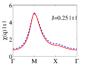
Figure 1: (Color online) Quasimomentum dependences of spin susceptibilities: calculation by the $t-J$ model according to Vladimirov07 (dashed line) and calculation by model susceptibility (26) (solid line). The chosen direction for rounding the Brillouin zone is $\Gamma(0,0)\rightarrow M(\pi,\pi)\rightarrow X(\pi,0)\rightarrow\Gamma(0,0)$.

With allowance for the above assumptions, we obtain, in the first Born approximation, that

$$\delta P(\textbf{k},i\omega_{m})=\frac{1}{N}\sum_{\textbf{q}}\frac{(t_{\textbf{q}}+J_{\textbf{k-q}})\chi(\textbf{q}-\textbf{k})\Omega_{SF}}{i\omega_{m}-\xi_{\textbf{q}}},$$ (28)

$$\Sigma(\textbf{k})=-\frac{1}{N}\sum_{\textbf{q}}(t_{\textbf{q}}+J_{\textbf{k-q}})n_{F}(\xi_{\textbf{q}}),$$ (29)

where $n_{F}(x)=(\exp(\frac{x-\mu}{T})+1)^{-1}$ is the Fermi–Dirac function. Then, expression (5) for the single-particle Green’s function acquires the form

$$D(\textbf{k},i\omega_{m})=\frac{C_{n}+\delta P(\textbf{k},i\omega_{m})}{i\omega_{m}-\xi_{\textbf{k}}-t_{\textbf{k}}\delta P(\textbf{k},i\omega_{m})-\Sigma(\textbf{k})}.$$ (30)

The obtained system should be added with the equation for chemical potential $\mu$

$$\frac{n}{2}=\frac{T}{N}\sum_{k,\omega_{m}}e^{i\omega_{m}\delta}D(\textbf{k},i\omega_{m}),~{}~{}~{}\delta\rightarrow\infty.$$ (31)

The spectral intensity of the system can be calculated after analytical continuation using expression (II).

IV Pseudogap behavior of the spectral intensity of Hubbard fermions

Fig. 2 presents spectral intensities $A(\textbf{k},\omega)$ of the model under consideration calculated for the electron density $n=0.95$ along the principle directions of the Brillouin zone (left plots) and on the Fermi contour for a quarter of the Brilouin zone (right plots). Here, the value of the spectral intensity is reflected by brightness of the energy spectrum lines (the lighter the line, the larger is the value $A(\textbf{k},\omega)$). The energy parameters of the model was measured in units $|t|$

$$T=0.01,~{}t=-1,~{}t^{\prime}=-0.65,~{}t^{\prime\prime}=-0.5,~{}J=0.25$$

and chosen such that the Fermi surface would have the form of pockets, in accordance with the experimental data on magnetic oscillations Doiron07 . The upper panel shows $A(\textbf{k},\omega)$ corresponding to the Hubbard-I approximation. In this case, the value of $A(\textbf{k},\omega)$ remains invariable at the change in the quasimomentum along the energy spectrum and at the Fermi surface. The middle panel demonstrates the results of the calculation of $A(\textbf{k},\omega)$ with regard to SFs. Comparison with the upper panel shows that the allowance for SFs results in the qualitative difference, specifically, the occurrence of considerable $A(\textbf{k},\omega)$ modulation both at the spectrum line and at the Fermi level. It can be seen that the value of $A(\textbf{k},\omega)$ decreases most in the wide energy region near the chemical potential.

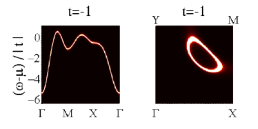
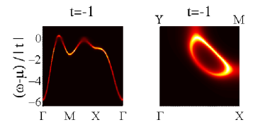
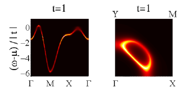
Figure 2: (Color online) Lines of the Fermi excitations and Fermi surfaces with allowance for the spectral intensity. The upper panel corresponds to the Hubbard-I approximation; the middle and lower panels, to allowance for SFs at different signs of hopping parameter $t$.

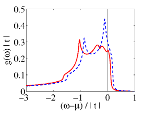
Figure 3: (Color online) Density of electron states calculated in the Hubbard-I approximation (dashed line) and with allowance for the spin-fluctuation processes (solid line). The vertical line reflects the position of the chemical potential.

Note an important feature related to the effect of the sign of $t$ on modulation of the spectral intensity. This feature is illustrated in the lower panel of Fig. 2, where the spectral intensity calculated for positive $t$ is shown. In the calculation, all the rest parameters of the system remained invariable. Comparison of the middle and lower panels of the figure shows that at negative $t$ the spectral intensity at the Fermi contour in maximum in the vicinity of the point $(\pi,\pi)$, whereas at $t>0$ the $A(\textbf{k},\omega)$ maximum at the Fermi contour is located on the opposite side of the pocket, i.e., at the contour fragment that is closer to the point $(0,0)$. Note that this case corresponds to the results of the ARPES experiments (see, for example, Hashimoto08 ).

The developed modification of the spectral intensity by the expense of the fluctuation processes qualitatively changes the density of electron states

$$g(\omega)=\frac{1}{N}\sum_{\textbf{k}}A(\textbf{k},\omega).$$ (32)

Fig. 3 illustrates the densities of states calculated in the Hubbard-I approximation (dashed line) and with allowance for SFs (solid line). Comparing the two curves, one can see that the allowance for the fluctuation processes results in the drastic reduction of the density of states in the vicinity of the chemical potential. Thus, the results of our analysis show the formation of the pseudogap state in the considered system of Hubbard fermions.

V Spectrum of Hubbard fermion excitations and the pseudogap behavior in the limit $U\rightarrow\infty$

In this Section, we thoroughly analyze the physical nature of modulation of the spectral intensity in the system of Hubbard fermions. To elucidate the key points, we consider a simplified problem allowing us to obtain analytical expressions for the Fermi energy spectrum and spectral intensity but, at the same time, preserving the fundamental features of Hubbard fermions. It is possible with the use of the Hubbard model (2) in the regime of extremely strong electron correlations ($U\rightarrow\infty$) when the Hamiltonian contains only the part corresponding to the operator of kinetic energy in the atomic representation ($t$ model)

$$\hat{H}=\hat{H}_{t}.$$ (33)

Note that, since the model is simplified down to the limit, the below results on the properties of the Fermi excitation spectrum cannot be applied to the description of the experimental ARPES data and are used only to explain clearly the physical nature of the modulation of the spectral intensity in the ensemble of Hubbard fermions. This approach is analogous, in a sense, to the way in which the idealized Kronig–Penney model Kronig31 illustrates the nature of the occurrence of energy bands in a crystal at the analysis of electron motion in a periodic potential.

To study the spectral properties of Hubbard fermions in the $t$ model, we use, as earlier, the method developed in Section II. In our case, the one-loop correction for $\delta P(\textbf{k},i\omega_{m})$ is determined only by the two upper plots from (13). The corresponding nonlinear integral equation for the strength operator will have the form

$$\delta P(\textbf{k},i\omega_{m})=\frac{T}{N}\sum_{\textbf{q},i\omega_{l}}\frac{t_{\textbf{q}}\,\chi(\textbf{q}-\textbf{k},i\omega_{l}-i\omega_{m})}{i\omega_{l}-\xi_{\textbf{q}}-t_{\textbf{q}}\,\delta P(\textbf{q},i\omega_{m})}.$$ (34)

Choosing the quasimomentum dependence for the spin susceptibility, we again take into account the experimental fact of the presence of a sharp peak of this function in the vicinity of the antiferromagnetic instability point $\textbf{Q}=(\pi,\pi)$ Hammel89 . However, unlike the previous case, now we obtain simplified analytical expressions considering the limiting situation where the peak of magnetic susceptibility is delta-like. Then, $\chi_{SF}(\textbf{q},0)$ is presented as

$$\chi_{SF}\left(\textbf{q},0\right)=\chi_{0}\cdot\delta(\textbf{q}-\textbf{Q}).$$ (35)

To determine the value of $\chi_{0}$, we use, as earlier, model susceptibility (27). Then, for the first Born approximation, we have

$$\delta P(\textbf{k},i\omega_{m})=\frac{\Omega_{SF}\chi_{0}t_{\textbf{k}+\textbf{Q}}}{i\omega_{m}-\xi_{\textbf{k}+\textbf{Q}}}$$ (36)

and expression (5) for the single-particle Green’s function acquires the two-pole structure

$$D(\textbf{k},i\omega_{m})=\frac{C_{n}+\delta P(\textbf{k},i\omega_{m})}{i\omega_{m}-\xi_{\textbf{k}}-t_{\textbf{k}}\delta P(\textbf{k},i\omega_{m})}=$$ (37)

$$=\frac{C_{n}(i\omega_{m}-\xi_{\textbf{k}+\textbf{Q}})+\Omega_{SF}\chi_{0}t_{\textbf{k}+\textbf{Q}}}{(i\omega_{m})^{2}+\xi_{\textbf{k}}\xi_{\textbf{k}+\textbf{Q}}-i\omega_{m}(\xi_{\textbf{k}}+\xi_{\textbf{k}+\textbf{Q}})-\Omega_{SF}\chi_{0}t_{\textbf{k}}t_{\textbf{k}+\textbf{Q}}}.$$

Hence, the allowance for SFs forms two branches of the Fermi excitation spectrum

$$E^{\pm}_{\textbf{k}}=C_{n}R_{\textbf{k}}\pm\sqrt{\left(C_{n}^{2}-\Omega_{SF}\chi_{0}\right)t_{1\textbf{k}}^{2}+\Omega_{SF}\chi_{0}R^{2}_{\textbf{k}}}.$$ (38)

The equation for chemical potential $\mu$ is

$$\frac{n}{2}=\frac{1}{N}\sum_{k}\Bigl{(}n_{F}(E^{+}_{\textbf{k}})A^{+}_{\textbf{k}}+n_{F}(E^{-}_{\textbf{k}})A^{-}_{\textbf{k}}\Bigr{)},$$ (39)

where the functions

$$A^{\pm}_{\textbf{k}}=\frac{1}{2}(C_{n}\pm\lambda_{\textbf{k}}),$$

$$\lambda_{\textbf{k}}=\frac{(C_{n}^{2}-\Omega_{SF}\chi_{0})t_{1\textbf{k}}+\Omega_{SF}\chi_{0}R_{\textbf{k}}}{\sqrt{\left(C_{n}^{2}-\Omega_{SF}\chi_{0}\right)t_{1\textbf{k}}^{2}+\Omega_{SF}\chi_{0}R_{\textbf{k}}^{2}}}$$ (40)

determine partial contributions of each branch of the spectrum to the total spectral intensity

$$A(\textbf{k},\omega)=A^{+}(\textbf{k},\omega)+A^{-}(\textbf{k},\omega),$$

$$A^{\pm}(\textbf{k},\omega)=A^{\pm}_{\textbf{k}}\delta(\omega-E^{\pm}_{\textbf{k}}).$$

As will be shown below, the change in the values of the $A^{\pm}_{\textbf{k}}$ functions at the change in k (for example, upon motion along the isoenergetic line) leads to the formation of significant modulation of $A(\textbf{k},\omega)$ as soon as SFs become strong.

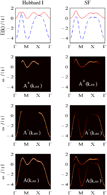
Figure 4: (Color online) Spectrum of the Fermi excitations along the principal directions of the Brillouin zone and modification of the spectral intensities with allowance for the spin-fluctuation processes.

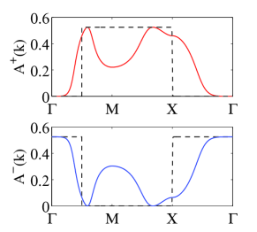
Figure 5: (Color online) Dependences of partial contributions to the spectral intensity on the quasimomentum with allowance for SFs (solid lines). For comparison, the dashed lines show the dependences of these functions in the Hubbard-I approximation.

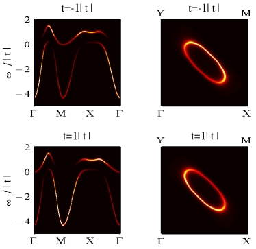
Figure 6: (Color online) Effect of the sign of hopping parameter $t$ on modulation of the spectral intensity.

The occurrence of $A(\textbf{k},\omega)$ modulation is illustrated in Fig. 4. The upper plot on the left presents the energy spectrum development in the limit of the vanishingly small power of SFs ($\Omega_{SF}\cdot\chi_{0}\rightarrow 0$) for the electron density $n=0.95$. As earlier, the values of the energy parameters of the model in the units of $|t|$

$$T=0.01,~{}t=-1,~{}t^{\prime}=-0.65,~{}t^{\prime\prime}=-0.4,$$ (41)

were chosen such that the Fermi surface would have the form of the pockets. The dashed line corresponds to the lower branch $E^{-}_{\textbf{k}}$ of the spectrum; the solid line, to the upper branch $E^{+}_{\textbf{k}}$. Despite there are two solutions of the dispersion equation, in reality the only branch is revealed. This is due to the fact that at $\Omega_{SF}\chi_{0}\rightarrow 0$ the partial contributions

$$A^{\pm}_{\textbf{k}}=\frac{1}{2}C_{n}\left\{1\pm\textrm{sign}(t_{1\textbf{k}})\right\}.$$ (42)

sharply grow from zero to the end value or sharply drop from the end value to zero at the variation in the quasimomentum (dashed lines in Fig. 5). Therefore, at each nonzero point of the Brillouin zone having the same value, only one of the partial spectral intensities $A^{\pm}(\textbf{k},\omega)$ may exist. The total $A(\textbf{k},\omega)$ spectral intensity (the values of these functions are reflected in the plots by thickness of the corresponding lines) remains invariable at the variation in the quasimomentum along the energy spectrum. In our simple case, this corresponds to the Hubbard-I approximation. The considered features are illustrated by the left plots of the second, third, and fourth panels in Fig. 4.

The situation becomes qualitatively different when SFs switch (right plots in Fig. 4). The upper right plot presents the spectra calculated at $\Omega_{SF}\chi_{0}=0.16$. As before, the solid line shows the $E^{+}_{\textbf{k}}$ spectrum; the dashed line, the spectrum $E^{-}_{\textbf{k}}$. Switching of the interaction between the electron subsystem with the subsystem of spin degrees of freedom via the kinematic mechanism leads to repulsion of the spectrum branches at the points where they were osculating without interaction.

The more significant effect of SFs is related to considerable modification of the spectral weights $A^{\pm}_{\textbf{k}}$, which manifests itself in strong renormalization of the values of these functions (Fig. 5). As a result, the partial spectral intensity $A^{+}(\textbf{k},\omega)$ acquires a finite value over the entire curve of the energy spectrum $E^{+}_{\textbf{k}}$ (similarly, $A^{-}(\textbf{k},\omega)$ is finite along the entire $E^{-}_{\textbf{k}}$ curve) and becomes strongly modulated. It can be clearly seen from comparison of the left and right plots in the second and third panels in Fig. 4. The total spectral intensity $A(\textbf{k},\omega)$ acquires the structure reflecting the presence of two branches exhibiting strong modulation. In the right plot of the lower panel in Fig. 4, the degree of darkening of the parts in the vicinity of the points $(\textbf{k},\omega)$ corresponds to the value of $A(\textbf{k},\omega)$ in these points. It can be seen that the allowance for SFs has led to induction of the shaded zone and redistribution of the spectral intensity between the basic and shaded zones.

The feature related to the change in the sign of parameter $t$ of hopping to the first coordination sphere (Fig.2) is characteristic of this model. Fig. 6 shows the spectral intensity calculated along the principle directions of the Brillouin zone (left plots) and at the Fermi contour for a quarter of the Brillouin zone (right plots) at different signs of $t$. It can be seen that, at $t>0$, $A(\textbf{k},\omega)$ is maximum in the part of the Fermi contour that is closer to the point $(0,0)$, which is consistent with the experimental data.

VI Summary

To sum up, we formulate the principles of the kinematic formation of modulation of the spectral intensity $A(\textbf{k},\omega)$. Of fundamental importance is the use of the faithful representation for a single-fermion Matsubara Green’s function $D(\textbf{k},i\omega_{m})$. For the kinematic mechanism, $D(\textbf{k},i\omega_{m})$ is expressed as the product of the propagator part and strength operator $P(\textbf{k},i\omega_{m})$. The presence of the strength operator in the numerator of the Green’s function and its dependence on the Matsubara frequency and quasimomentum lead to the fact that the isoenergetic lines in the quasimomentum space become different from the lines where the strength operator has a constant value. This spacing is one of the causes of modulation of the spectral intensity $A(\textbf{k},\omega)$. It is important that the integral of hopping to the first coordination sphere determines the Fermi contour part where $A(\textbf{k},\omega)$ considerably decreases.

The specific cause of $A(\textbf{k},\omega)$ modulation in the framework of the kinematic interaction is that SFs lead to the formation of a shaded zone, which represents the initial zone shifted in the quasimomentum space by the vector $(\pi,\pi)$. As a result, the total pattern of the spectrum is formed by coherent hybridization of these two zones, between which the spectral intensity is redistributed and, consequently, the density of states in the vicinity of the chemical potential drops.

To demonstrate the kinematic formation of the pseudogap behavior as brightly as possible, we considered the Hubbard model in the limit of strong correlations when the dynamics of Hubbard fermions is governed by the kinematic interaction. Obviously, the discovered mechanism of the pseudogap phase formation is universal and relevant for other models of strongly correlated systems.

- (1) T. Timusk and B. Statt, Rep. Prog. Phys. 62, 61 (1999).
- (2) M. V. Sadovskii, Phys. Usp. 44, 515 (2001).
- (3) A. Damascelli, Z. Hussain, and Z.-X. Shen, Rev. Mod. Phys. 75, 473 (2003).
- (4) S. Chakravarty, L. B. Laughlin, D. K. Morr, and C. Nayak, Phys. Rev. B 63, 094503 (2001).
- (5) M. E. Simon and C. M. Varma, Phys. Rev. Lett. 89, 247003 (2002).
- (6) K.-Y. Yang, T. M. Rice, and F.-C. Zhang, Phys. Rev. B 73, 174501 (2006).
- (7) P. W. Anderson, Science 235, 1196 (1987).
- (8) J. P. F. LeBlanc, E. J. Nicol, and J. P. Carbotte, Phys. Rev. B 80, 060505(R) (2009).
- (9) J. P. Carbotte, K. A. G. Fisher, J. P. F. LeBlanc, and E. J. Nicol, Phys. Rev. B 81, 014522 (2010).
- (10) E. Schachinger and J. P. Carbotte, Phys. Rev. B 81, 214521 (2010).
- (11) A. J. H. Borne, J. P. Carbotte, and E. J. Nicol, Phys. Rev. B 82, 024521 (2010).
- (12) J. P. Carbotte, Phys. Rev. B 83, 100508(R) (2011).
- (13) A. Pound, J. P. Carbotte, and E. J. Nicol, Eur. Phys. J. B 81, 69 (2011).
- (14) K.-Y. Yang, H. B. Yang, P. D. Johnson, T. M. Rice, and F.-C. Zhang, Europhys. Lett. 86, 37002 (2009).
- (15) Th. A. Maier, Th. Pruschke, and M. Jarrell, Phys. Rev. B 66, 075102 (2002).
- (16) F. F. Assaad, M. Imada, and D. J. Scalapino, Phys. Rev. B 56, 15001 (1997).
- (17) B. Kyung, J.-S. Landry, and A.-M. S. Tremblay, Phys. Rev. B 68, 174502 (2003).
- (18) M. V. Sadovskii, I. A. Nekrasov, E. Z. Kuchinskii, Th. Pruschke, and V. I. Anisimov, Phys. Rev. B 72, 155105 (2005).
- (19) E. Z. Kuchinskii, I. A. Nekrasov, and M. V. Sadovskii, Phys. Rev. B 75, 115102 (2007).
- (20) W. Stephan and P. Horsch, Phys. Rev. Lett. 66, 2258 (1991).
- (21) R. Preuss, W. Hanke, C. Gröber, and H. G. Evertz, Phys. Rev. Lett. 79, 1122 (1997).
- (22) J. C. Hubbard, Proc. R. Soc. London A 276, 238 (1963).
- (23) D. Zanchi and H. J. Schulz, Europhys. Lett. 44, 235 (1997).
- (24) N. Furukawa, T. M. Rice, and M. Salmhofer, Phys. Rev. Lett. 81, 3195 (1998).
- (25) J. Schmalian, D. Pines, and B. Stojković, Phys. Rev. Lett. 80, 3839 (1998); Phys. Rev. B 60, 667 (1999).
- (26) A. V. Chubukov and D. K. Morr, Phys. Rep. 288, 355 (1997).
- (27) P. Monthoux, A. V. Balatsky, and D. Pines, Phys. Rev. Lett. 67, 3448 (1991); Phys. Rev. B 46, 14803 (1992); P. Monthoux and D. Pines, Phys. Rev. B 47, 6069 (1993).
- (28) T. Dahm, D. Manske, and L. Tewordt, Phys. Rev. B 60, 14888 (1999).
- (29) P. Prelovšek and A. Ramšak, Phys. Rev. B 63, 180506(R) (2001); 65, 174529 (2002).
- (30) N. M. Plakida and V. S. Oudovenko, JETP 104, 230 (2007).
- (31) D. N. Zubarev, Phys. Usp. 3, 320 (1960).
- (32) H. Mori, Prog. Theor. Phys. 33, 423 (1965).
- (33) J. C. Hubbard, Proc. R. Soc. London A 285, 542 (1965).
- (34) F. J. Dyson, Phys. Rev. 102, 1217 (1956); 1230 (1956).
- (35) R. O. Zaitsev and V. A. Ivanov, Sov. Phys. Solid State 29, 1475 (1987).
- (36) R. O. Zaitsev, Sov. Phys. JETP 41, 100 (1975); 43, 574 (1976).
- (37) R. O. Zaitsev, Diagram Methods in the Theory of Superconductivity and Magnetism (Editorial URSS, Moscow, 2004) [in Russian].
- (38) V. G. Bar yakhtar, V. E. Krivoruchko, and D. A. Yablonsky, Green s Functions in the Theory of Magnetism (Naukova Dumka, Kiev, 1984) [in Russian].
- (39) S. G. Ovchinnikov and V. V. Val’kov, Hubbard Operators in the Theory of Strongly Correlated Electrons (Imperial College Press, London, 2004).
- (40) V. V. Val’kov and A. A. Golovnya, JETP 107, 996 (2008).
- (41) A. F. Barabanov and O. A. Starykh, J. Phys. Soc. Jpn. 61, 704 (1992).
- (42) N. M. Plakida and V. S. Oudovenko, Phys. Rev. B 59, 11949 (1999).
- (43) J. Hubbard and K. P. Jain, J. Phys. C (Proc. Phys. Soc.) 1, 1650 (1968).
- (44) H. Shimahara and S. Takada, J. Phys. Soc. Jpn. 61, 989 (1992).
- (45) A. A. Vladimirov, D. Ihle, and N. M. Plakida, Teor. Math. Phys. 152, 1331 (2007).
- (46) M. V. Eremin, A. A. Aleev and I. M. Eremin, JETP 106, 752 (2008).
- (47) P. C. Hammel, M. Takigawa, R. H. Heffner, et al., Phys. Rev. Lett. 63, 1992 (1989).
- (48) N. M. Plakida, L. Anton, S. Adam, and G. Adam, JETP 97, 331 (2003).
- (49) J. Jaklič and P. Prelovšek, Phys. Rev. Lett. 74, 3411 (1995); 75, 1340 (1995).
- (50) N. Doiron-Leyraud, C. Proust, D. LeBoeuf, et al., Nature 447, 565 (2007).
- (51) M. Hashimoto, T. Yoshida, H. Yagi et al., Phys. Rev. B 77, 094516 (2008).
- (52) R. de L. Kronig and W. G. Penney, Proc. R. Soc. London A 130, 499 (1931).