Parallel and Perpendicular Susceptibility Above $T_{c}$ in La_2-xSr_xCuO₄ Single Crystals

Abstract

We report direction-dependent susceptibility and resistivity measurements on La_2-xSr_xCuO₄ single crystals. These crystals have rectangular needle-like shapes with the crystallographic “c” direction parallel or perpendicular to the needle axis, which, in turn, is in the applied field direction. At optimal doping we find finite diamagnetic susceptibility above $T_{\mathbf{c}}$, namely fluctuating superconductivity (FSC), only when the field is perpendicular to the planes. In underdoped samples we could find FSC in both field directions. We provide a phase diagram showing the FSC region, although it is sample dependent in the underdoped cases. The variations in the susceptibility data suggest a different origin for the FSC between underdoping (below $10\%$) and optimal doping. Finally, our data indicates that the spontaneous vortex diffusion constant above $T_{c}$ is anomalously high.

The superconducting and ferromagnetic phase transitions share a lot in common, but it is simpler to visualize the latter. The magnetic moment direction in a ferromagnet is analogous to the phase of the superconducting order parameter, and the magnetic field produced by the ferromagnet is equivalent to the lack of resistance of a superconductor. A ferromagnet produces a maximal magnetic field when all its domains are aligned. Similarly, a superconductor has no resistance only if the phase of the order parameter is correlated across the entire sample. However, a ferromagnet can have local magnetization, without global alignment of domains. Similarly, a superconductor can have local superconductivity, manifested in diamagnetism, without zero resistance across the entire sample. This situation is the hallmark of fluctuating superconductivity without global phase coherence. In a two dimensional system, where long range-order is forbidden Mermin , the role of domains is played by a vortex anti-vortex pair, which breaks the fabric of the phase. Detecting fluctuating superconductivity in a particular compound is essential for understanding the structure of its phase transition.

In the highly anisotropic cuprate superconductors, the presence of diamagnetism well above the resistance critical temperature, $T_{c}$, was demonstrated some time ago, with high magnetic field $H$ perpendicular to the superconducting planes TorronPRB94 ; LuLi . This finding was, indeed, interpreted as persistence of the finite order parameter amplitude throughout the sample, but with short-range phase coherence above $T_{c}$. However, a completely different interpretation could be offered to the same effect, in which electrons are inhomogeneously localized due to the randomness of the dopant. There are several experimental indications for inhomogeneous localization Localization . In this case, superconductivity can occur with finite order parameter amplitude only in three dimensional patches of the sample, leading to a local diamagnetic signal without a continuous resistance-free path at $T>T_{c}$. In the localization scenario, a diamagnetic signal should be detected above $T_{c}$ for all directions of the applied field $H$.

In this work, we examine the fluctuating superconductivity of La_2-xSr_xCuO₄ using magnetization ($M$) measurements with the field parallel and perpendicular to the CuO₂ planes. We work in the zero field limit, as required by the definition of susceptibility. We also perform resistivity measurements on the exact same samples. Our major finding, summarized in Fig. 1, is a diamagnetic susceptibility in the resistive phase of highly underdoped sample, for both the parallel and perpendicular field, supporting the localization scenario. Close to optimal doping, a diamagnetic signal in the resistive phase exists only when the field is perpendicular to the superconducting planes, in accordance with the phase fluctuation scenario.

We generate a phase diagram in Fig. 2 showing, for each doping, the temperatures at which resistivity vanishes, and the temperatures at which a diamagnetic signal appears for different field directions. We also compute the spontaneous vortex diffusion constant $D=\chi_{C}\rho_{ab}/\mu_{0}$ using our DC data and find it to be anomalously high. The implications of such high $D$ are discussed in Ref. 6.

The paper is organized as follows. In Sec. I we describe the experiment. In Sec. II we present our major findings in more details. We clarify which experimental variables are relevant for our findings in Sec. III using several control experiments. Finally, in Sec. IV we summarize our conclusions.

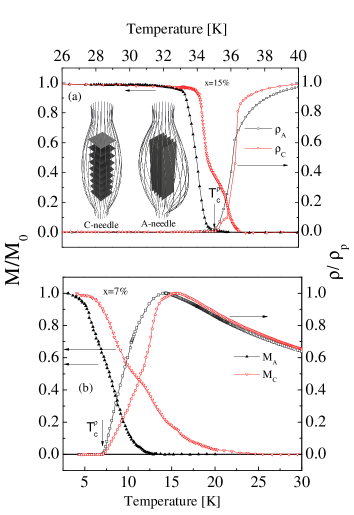
Figure 1: LSCO normalized magnetization (left axis) and resistivity (right axis) measurements as a function of temperature of (a) optimally doped ($x=15\%$) and (b) underdoped ($x=7\%$) samples in an applied field of $H=0.5$ Oe for two types of sample: A- and C-needles. In these needles, the superconducting planes are parallel or perpendicular to the needle direction, respectively. The magnetic field is applied along the needles, and field lines wrap the samples. The A-needle is $1\times 1\times 10$ mm³ and the C-needle is $1\times 1\times 5$ mm³. $M_{0}$ is the magnetization at zero temperature and $\rho_{p}$ is the resistivity at the peak. $T_{c}^{\rho}$ indicates zero resistivity.

I Experimental Details

In magnetization experiments in the zero field limit, the measured susceptibility $\chi_{m}=\lim_{H\rightarrow 0}M/H$ depends on the sample geometry via the demagnetization factor ($D$), and is given by ${\chi_{m}=\chi_{i}/(1+D\chi_{i})}$ where $\chi_{i}$ is the intrinsic susceptibility. For needle-like samples, $D\simeq 0$ and $\chi_{m}=\chi_{i}$. Therefore, in order to determine $\chi_{i}$ properly needle-like samples are needed. To achieve the $D\simeq 0$ condition we utilize rod-like La_2-xSr_xCuO₄ single crystals grown in an image furnace, which are oriented with a Laue camera and a goniometer. After the orientation, the goniometer with the rod is mounted on a saw and needle shaped samples are cut. Two configurations are produced as shown in Fig. 1. These crystals have rectangular needle-like shapes with the crystallographic “c” direction parallel (C-needle) or perpendicular (A-needle) to the needle axis.  We were able to prepare 10 mm-long A-needles and only 5 mm-long C-needles. Unless stated otherwise, the needles have $1\times 1$ mm² cross-section. The field is applied along the needle axis direction. Field lines, expelled from the sample as in the superconducting state, are also shown in Fig. 1. For each sample we performed direction-dependent susceptibility and resistivity measurements. The measurements are carried out in zero field cooling conditions using a Cryogenic SQUID magnetometer equipped with a low field power supply with a field resolution of 0.01 Oe. Prior to each measurement batch, the external field is zeroed with a Type I SC.

II Major Findings

Figure 1(a) and (b) demonstrate our major finding. In this figure we depict the normalized magnetization $M/M_{0}$ as a function of $T$, at a field of $H=0.5$ Oe, for the $x=15\%$ and $7\%$ samples respectively, for two different orientations. $M_{A}$ and $M_{C}$ are measurements performed on the A- and C-needle, respectively. $M_{C}$ shows a knee upon cooling. This knee exists in all C-needle measurements but its size and position appears to be random. Resistivity data, normalized to 1 at the peak, are also presented in this figure; $\rho_{A}$ and $\rho_{C}$ are the resistivities measured using the corresponding needles with the contacts along the needles. The resistivity results are similar to those previously reported KomiyaPRB02 . The superconducting transition of the $7\%$ sample is wide. However, it is known that $8\%$ and higher doping samples are superconductors, and $5\%$ and lower doping samples are insulators KomiyaPRB02 . Therefore, it is not surprising that the resistivity of a $7\%$ sample has a broad transition.

There is a small difference in the temperature at which zero resistivity appears, as determined by $\rho_{A}$ or $\rho_{C}$. We define the critical temperature $T_{c}^{\rho}$ as the smaller of the two. In contrast, a clear anisotropy is evident in the temperature at which the magnetization is detectable; this difference increases as the doping decreases. For the $15\%$ sample: $M_{A}$ is not detectable above $T_{c}^{\rho}=35~{}$K, but $M_{C}$ is finite up to $36.5~{}$K. The critical temperature of the material $T_{c}$ could be defined by one of two criteria: $T_{c}^{\rho}$, or the presence of three dimensional diamagnetism (finite $M_{A}$). For the $15\%$ sample, the difference in $T_{c}$ between the two criteria is on the order of our measurement accuracy discussed in Sec. III. The strong residual $M_{C}$ above $T_{c}^{\rho}$ without residual $M_{A}$ was never detected before in such low fields. It could result from decoupled superconducting planes disordered by vortices.

In contrast, for the $7\%$ case, both $M_{A}$ and $M_{C}$ are finite at temperatures well above $T_{c}^{\rho}=7.0$ K. $M_{A}$ is not detectable only above $13~{}$K and $M_{C}$ is finite up to $25~{}$K. The sharpest transition is observed with the $M_{A}$ measurement; this type of measurement could be used to define doping and sample quality. The dramatic difference between the $15\%$ and $7\%$ doping indicates that the fluctuating superconductivity above $T_{c}^{\rho}$ at low doping is fundamentally different from optimal doping, and could be derived by electronic inhomogeneous localization.

The DC in-plane resistivity for the 7% and 15% samples is $\rho_{ab}=2.5\times 10^{-4}$ and $0.5\times 10^{-5}$ $\Omega$-cm respectively, at the crossing point between the resistivity $\rho_{A}$ and the magnetization $M_{c}$ curves KomiyaPRB02 . The volume susceptibility of the 7% and 15% needles, also at the crossing point, is 0.48 and 0.12 of the saturation value respectively (see Fig. 1). This leads to an anomalously high spontaneous vortex diffusion constant $D=\chi_{C}\rho_{ab}/\mu_{0}\sim 10^{4}$ and $10^{2}$ cm²/sec for the 7% and 15%; which is much higher than previously reported BilbroPRB11 .

We repeat the same measurements for several different dopings. For each doping we determine three temperatures: $T_{M}^{C}$ and $T_{M}^{A}$ are the temperatures at which the magnetization of the $C$- and $A$-needles become finite, and $T_{c}^{\rho}$. The three temperatures are plotted as a function of doping in Fig. 2. On the scale of the figure, $T_{c}^{\rho}$ and $T_{M}^{A}$ are very close to each other for all doping, and are different from $T_{M}^{C}$. The difference between $T_{M}^{C}$ and both $T_{c}^{\rho}$ and $T_{M}^{A}$ is small and roughly constant for doping higher than 10%, with the exception of the stripe ordered phase at 1/8 doping. Interestingly, at this phase $T_{M}^{C}$ follows the general trend, while $T_{M}^{A}$ and $T_{c}^{\rho}$ are suppressed as if the stripes are affecting the interlayer coupling only. Below 10% this difference increases upon underdoping.

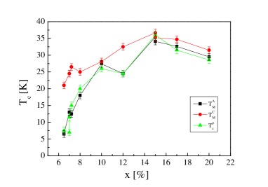
Figure 2: Doping dependence of the superconducting critical temperature determined by the zeroing of resistivity $T_{c}^{\rho}$ and the temperature at which a diamagnetic signal appears in magnetization measurements for C-needle $T_{M}^{C}$ and A-needle $T_{M}^{A}$.

III Control Experiments

In order to verify these results we perform several control experiments. First we examine the influence of the field on the susceptibility. In Fig. 3 (a) and (b) we plot $4\pi\chi_{m}$ for the 15% $C$- and $A$-needles respectively, as a function of temperatures, and for several applied magnetic fields. For the field range presented, the saturation value of the susceptibility is field-independent. At $T\rightarrow 0$, $4\pi\chi_{m}=-1.1$ and $-1.0$ for the $C$- and $A$-needles, respectively. For our rectangular $C$-needle, with dimensions of $1\times 1\times 5$ mm³, the demagnetization factor is $D\simeq 4\pi\times 0.09$, which explains well the measured susceptibility. For our rectangular $A$-needle with dimensions of $1\times 1\times 10$ mm³, $D\simeq 4\pi\times 0.045$ and we expect $4\pi\chi_{m}=-1.05$, which is slightly higher than the observed value demagnetization1 . A more accurate analysis of the susceptibility of needles is given below. At the other extreme, when $T\rightarrow T_{c}$ we see field-dependent susceptibilities but only for fields higher than 1 Oe. Below 1 Oe, $\chi_{m}(T)$ converges to a field-independent function representing the zero field susceptibility. Therefore, all our measurements are done with a field of 0.5 Oe. Finally, the knee exists in the $M_{C}(T)$ data only for fields lower than 10 Oe.

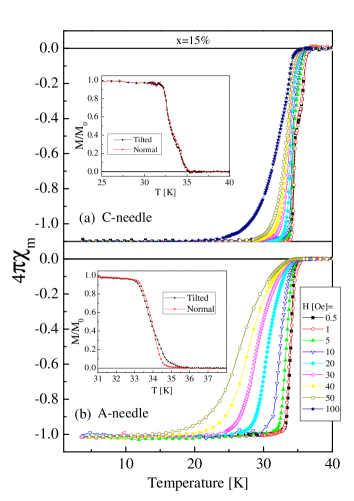
Figure 3: The measured susceptibility $\chi_{m}$ ($\equiv M/H$) as a function of temperature for the 15% (a) C-needle and (b) A-needle in various magnetic fields. Insets: measurements of a straight and tilted needles demonstrating the effect of misalignment.

In Fig. 4 we provide the field dependence of the susceptibility for the 7% needles. Here again, the susceptibility converges into a field-independent function at $H\rightarrow 0$, especially close to $T_{c}$.

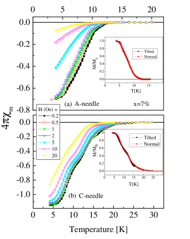
Figure 4: The measured susceptibility $\chi_{m}$ ($\equiv M/H$) as a function of temperature for the 7% (a) C-needle and (b) A-needle in various magnetic fields. Insets: measurements of a straight and tilted needles demonstrating the effect of misalignment.

We also examine the relevance of misalignment of the samples to our results by purposely tilting the needles by 7^∘. The measurements of a straight sample and a tilted one are shown in the insets of Fig. 3 and 4. Misalignment can lead to an error of 0.1 K per $1^{\circ}$ in the estimate of the temperature at which the magnetization is null. This tiny effect again cannot account for the difference in the magnetization between the A- and C-needles. In addition, the tilt does not affect the knee.

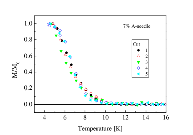
Figure 5: Magnetization as a function of temperature measurements performed on 5 different pieces cuts from the 7% A-needle. The pieces were ground into powder.

To test the doping homogeneity of the grown crystal, we cut the 7% A-needle into 5 pieces, grinned them into powder to remove shape-dependent effects, and measure the magnetization of each piece. The data are presented in Fig. 5. Judging from the scatter of points at half of the full magnetization, there is a scatter in $T_{c}$ of 2 K between the different pieces. This is much smaller than the difference between $T_{M}^{C}$ and $T_{M}^{A}$. Therefore, the difference between $T_{M}^{C}$ and $T_{M}^{A}$ is not a result of using two different pieces of sample for each measurement.

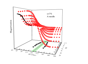
Figure 6: A 3D plot of the magnetization as a function of magnetic field and temperature for the 7% $A$-needle. (floor): $H_{c1}$ as a function of temperature. (wall): Magnetization as a function of $T$. The green solid line on the floor represents the applied field used in Fig. 1

Another concern is vortices. At a certain temperature close to $T_{c}$, the critical field $H_{c1}$ must drop below the applied magnetic field and vortices can enter the sample. This puts a limit on the range of temperature where interpreting our data is simple. Therefore, it is important to understand the behavior of $H_{c1}$ near $T_{c}$. Figure 6 shows the results of $M(H,T)$ for $x=7\%$ A-needle using a 3D plot. The values of $H_{c1}$ are determined by fitting $M(H)$ to a straight line around $H=0$ (not shown), and extracting the field where the linearity breaks. $H_{c1}(T)$ is shown on the floor of the plot. The applied field, depicted as the straight green line on the floor, is lower than $H_{c1}$ up to 12 K. At higher temperatures, vortices can enter the sample.

The measurements of $H_{c1}$ for the other samples and directions are depicted in Fig. 7. As long as $H_{c1}>0.5$ Oe the sample is free of vortices. In particular, this condition holds for the $7\%$ C-needle up to 20 K [see Fig. 7(c)] . This finding rules out the possibility that the knee observed in our C-needle measurements at fields lower than 10 Oe are due to a lock-in unlock-in transition of flux lines Lockin . The knees of the $7\%$ C-needle occur at temperatures of $15$ K at which the applied field is well below $H_{c1}$ and no vortices exist in the sample. With the lock-in mechanism ruled out, we can only speculate that the knees are due to the corners and edges of the sample. Put differently, if a C-needle could be polished into a long oval object without cleaving it, then the knee should have disappeared.

Figure 7: $H_{c1}$ as a function of temperature measured on (a) 15% A-needle (b) 15% C-needle (c) 7% C-needle.

Also, we investigate the impact of the sample geometry on the magnetization. Our motivation is to change the needle’s dimensions in terms of length-to-width ratio while maintaining needle-like aspect ratio. In Fig. 8, we present a multitude of $15\%$ measurements for A- and C-needles. The inset is a zoom close to $T_{c}$. The details of the magnetization curve are shape-dependent. However, the $2\times 2\times 10$ mm³ and $1\times 1\times 5$ mm³ A-needles have the same curve, demonstrating that the length-to-width ratio is the most significant parameter. The closer the samples are to an ideal needle-like form, the larger the difference in the magnetization between directions. This, of course, is expected since for a cubic or a spherical geometry, field lines cross the planes at an angle thus mixing the two susceptibilities leading to indistinguishable susceptibilities close to $T_{c}$ Panagopoulos .

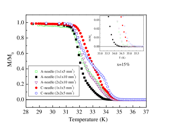
Figure 8: Magnetization versus temperature for several 15% A- and C-needles with different sample dimensions. Inset: A zoom-in close to the transition temperature.

Similar data for the 7% samples are given in Fig. 9. However, the 7% sample are not ideal for testing the impact of geometry on the magnetization. Each sample presented in the figure is cut from a different segment of the rod, which are a few centimeters apart. Since 7% doping is on the edge of the superconducting dome, small changes in the preparation conditions may lead to a severely different behavior, such as $T_{c}$ variations of $\sim 2$ K (see Fig. 5). Consequently, in Fig. 9 not only the geometry varies. In contrast, $T_{c}$ of the 15% samples is not sensitive to small doping variations.

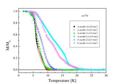
Figure 9: Magnetization versus temperature for several 7% A- and C-needles with different sample dimensions.

Finally, we examine the reproducibility of our most striking result, namely, the observation that for the 7% A-needle $T_{c}^{\rho}<T_{M}^{A}<T_{M}^{C}$. This test is done by growing a new crystal, cutting new A- and C- needles, and repeating the measurement. The result is shown in Fig. 10. This figure should be compared with Fig. 1(b). We find differences in many aspects between the first and second 7% samples. For example, the knee and the exact values of the critical temperatures. Nevertheless: (I) the order of temperatures $T_{c}^{\rho}<T_{M}^{A}<T_{M}^{C}$ which is the main focus of this work is maintained, and (II) the value of the susceptibility at the crossing point is $\sim 0.3$ of the saturation value, similar to the first 7% sample.

Figure 10: Reproducibility test using a second 7% crystal Both resistivity and magnetization are shown. The data should be compared with the original 7% crystal depicted in Fig. 1(b).

All these tests support our observation that the magnetization of the A- and C-needle are fundamentally different by an amount larger than any possible experimental error. One might try to explain these differences as a finite size effect, namely, as the penetration depth diverges when $T\rightarrow T_{c}$, it might have different values for each of the two different directions. Our magnetometer detects a diamagnetic signal only when the penetration depth is similar to the sample width. This could occur at different temperatures, which also differ from $T_{c}^{\rho}$.

To address this possibility, we examine the London penetration depth ($\lambda$) in our original $7\%$ sample (Fig. 1). In C-needle measurements, the screening currents run in the $ab$ planes and the susceptibility is sensitive to the in-plane penetration depth $\lambda_{ab}$. In contrast, in the $A$-needle measurements, the screening currents run both in- and between-planes. Therefore, the susceptibility is sensitive to both $\lambda_{ab}$ and the penetration length between planes $\lambda_{c}$. To extract these $\lambda$’s we solve an anisotropic London equation

$${b_{A}-\lambda_{ab}^{2}{\frac{{{\partial^{2}}b_{A}}}{{{\partial}x}^{2}}}-\lambda_{c}^{2}{\frac{{{\partial^{2}}b_{A}}}{{{\partial}y}^{2}}}}{=0}$$ (1)

$${b_{C}-\lambda_{ab}^{2}{\frac{{{\partial^{2}}b_{C}}}{{{\partial}x}^{2}}}-\lambda_{ab}^{2}{\frac{{{\partial^{2}}b_{C}}}{{{\partial}y}^{2}}}}{=0}$$ (2)

with the boundary condition $b_{\alpha}=1$, where $b_{A}$ and $b_{C}$ are the internal field divided by the applied field in the $A$- and $C$-needles respectively London . We define $\left\langle b_{\alpha}\right\rangle$ as the cross section average of $b_{\alpha}$. For the A-needle we find

$$\left\langle b_{A}\right\rangle = \sum_{n\text{ odd}}^{\infty}\left\{\frac{2/\sinh(\beta_{n}g)-2/\tanh(\beta_{n}g)+\beta_{n}g}{gj^{2}\beta_{n}^{3}/8}\right.$$

$$+\left.\frac{2/\sinh(\mu_{n}j)-2/\tanh(\mu_{n}j)+\mu_{n}j}{jg^{2}\mu_{n}^{3}/8}\right\}$$

where $g=w_{y}/\lambda_{c}$, $j=w_{x}/\lambda_{ab}$, $\beta_{n}=\sqrt{\left(\frac{\pi n}{j}\right)^{2}+1}$ , $\mu_{n}=\sqrt{\left(\frac{\pi n}{g}\right)^{2}+1}$, and $w_{x/y}$ is the sample width taken as 1 mm. $\left\langle b_{C}\right\rangle$ is obtained from Eq. III by $\lambda_{c}\rightarrow\lambda_{ab}$. The susceptibility is given by $\chi_{\alpha}=(\left\langle b_{\alpha}\right\rangle-1)/4\pi$. This provides an analytical solution for $\chi_{C}(\lambda_{ab})$ and $\chi_{A}(\lambda_{ab},\lambda_{c})$.

We obtain $\lambda_{ab}$ by equating the analytical solution to the measured susceptibility of the $C$-needle. We then substitute this $\lambda_{ab}$ into $\chi_{A}$ and extract $\lambda_{c}$ by equating the analytical solution to the measured susceptibility of the $A$-needle. Figure 11 depicts the calculated $\lambda_{ab}(T)$ and $\lambda_{c}(T)$ for $x=7\%$. The analysis is valid only far from magnetic saturation. Two arrows show the temperature where $H_{c1}$ is on the order of our measurement field ($0.5$ Oe). Eq. 1 is valid at temperatures lower than indicated by the arrows. It is also clear that the magnetization is finite when the penetration depth reaches the sample’s dimensions.

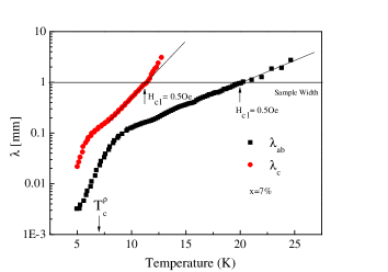
Figure 11: A semi log plot of the penetration depths $\lambda_{ab}$ and $\lambda_{c}$, as a function of $T$ obtained by comparing the analytical solutions of Eq. 1 and 2 with the measured susceptibilities of the original 7% sample presented in Fig. 1. The horizontal line represents the sample width. The points at which $H_{c1}$, for each needle, equals the applied field are also shown by arrows.

The surprising result is that $\lambda_{ab}$ and $\lambda_{c}$ run away from each other as the sample is warmed beyond $T_{c}^{\rho}$, and both reach the sample dimensions well above $T_{c}^{\rho}$. Therefore, had it been possible to increase the samples thickness, while maintaining needle-like geometry, a larger difference between the temperature of zero magnetization and $T_{c}^{\rho}$ would be expected, in contrast to a finite size scenario.

IV Discussion and Conclusions

It is important to mention other experimental and theoretical work showing a strong anisotropy in the temperature at which signals can be detected in LSCO. For example, Tranquada et al. TranquadaPRL07 measured the temperature dependence of $\rho_{ab}$ and $\rho_{c}$ with applied magnetic fields up to 9 T in a La_2-xBa_xCuO₄ single crystal with $x=9.5\%$. When $H$ was applied perpendicularly to the planes, it significantly suppressed the temperature at which $\rho_{c}\rightarrow 0$ without affecting $\rho_{ab}$. Thus, the field generated two effective $T_{c}^{\rho}$’s. Similarly, Schafgans et al. BasovPRL10 performed optical measurements in LSCO while applying a magnetic field up to 8 T parallel to the crystal c-axis. They found a complete suppression of the inter-plane coupling, while the in-plane superconducting properties remained intact. In addition, it was recently suggested theoretically that two dimensional-like superconductivity could be generated by frustration of the inter-layer coupling induced by stripes BergPRL07 , or by c-axis disorder PekkerPRL10 . These experiments and theories show that seemingly two different critical temperatures are conceivable.

In this work we examine the anisotropy of the susceptibility in La_2-xSr_xCuO₄ single crystals cut as needles. We find a different magnetic critical temperatures for measurements in two different directions. We also observe a diamagnetic susceptibility above $T_{c}^{\rho}$ for $H\|\mathbf{c}$ at all doping, and a diamagnetic susceptibility above $T_{c}^{\rho}$ for both $H\|\mathbf{c}$ and $H\bot\mathbf{c}$ at low doping. We suggest that at doping lower than 10%, electronic inhomogeneous localization is leading to local 3D superconducting patches, which provide diamagnetism without global superconductivity. Above 10% doping, vortices in an otherwise phase coherent state are responsible for finite resistivity coexisting with a diamagnetic signal in the $H\|\mathbf{c}$ case. Our experimental configuration allows us to calculate the spontaneous vortex diffusion constant using DC measurements. It is found to be much higher than previously thought BilbroPRB11 .

We also provide a phase diagram showing $T_{c}^{\rho}$ and the temperature at which a diamagnetic signal appears for each direction. At doping higher than 10%, our data support the existence of fluctuating superconductivity only a few degrees above $T_{c}^{\rho}$, namely, on a temperature scale much smaller than the pseuodogap scale. This is in contrast to high field measurements LuLi ; PatrickNatPhy11 , but in agreement with low field experiments TorronPRB94 ; GrbicPRB11 . How the field affects the temperature range of superconducting fluctuations, and whether this range is related to disorder or frustrations remains an open question.

V Acknowledgments

We acknowledge helpful discussions with N. Peter Armitage. This work was supported by the Israeli Science Foundation, by the Nevet program of the RBNI center for nano-technology, and by the Posnansky research fund in high temperature superconductivity.

References

- (1) N. D. Mermin and H. Wagner, Phys. Rev. Lett. 17, 1133 (1966).
- (2) C. Torrón, A. Díaz, A. Pomar, J. A. Veira, and F. Vidal, Phys. Rev. B 49, 13143 (1994).
- (3) Y. Wang, L. Li, M. J. Naughton, G. D. Gu, S. Uchida, and N. P. Ong, Phys. Rev. Lett. 95, 247002 (2005); Lu Li, Yayu Wang, M. J. Naughton, S. Ono, Yoichi Ando, and N. P. Ong, Europhys. Lett. 72, 451-457 (2005); Lu Li, Yayu Wang, Seiki Komiya, Shimpei Ono, Yoichi Ando, G. D. Gu and N. P. Ong, Phys. Rev. B 81, 054510 (2010).
- (4) G. S. Boebinger et al., PRL 77, 5417 (1996); J. Hori, S. Iwata, H. Kurisaki, F. Nakanura, T. Suzuki, and T. Fuhita, J. Phys. Soc. Jpn. 71 (2002) 1346; S. Komiya and Y. Ando, PRB 70 (2004) 060503(R).
- (5) S. Komiya, Y. Ando, X. F. Sun, and A. N. Lavtov, Phys. Rev. B 65, 214535 (2002). Y. Ando, S. Komiya, K. Segawa, S. Ono, and Y. Kurita, Phys. Rev. Lett. 93, 267001 (2004).
- (6) L. S. Bilbro, R. Valdés Aguilar, G. Logvenov, I. Bozovic, and N. P. Armitage, Phys. Rev. B 84, 100511(R) (2011).
- (7) M. Sato and Y. Ishii J. Appl. Phys. 66, 983 (1989).
- (8) D. Feinberg et al., Phys. Rev. Lett. 65, 919 (1990) ; V. Vulcanescu et al., Phys. Rev. B 50 4139 (1994); P.A. Mansky et al., Phys. Rev. B 52 7554 (1995); Yu.V. Bugoslavsky et al., Phys. Rev. B 56, 5610 (1997) ; Y. Bruckental et al.,, Phys. Rev. B 73, 214504 (2006).
- (9) C. Panagopoulos et al., Phys. Rev. B 53, R2999 (1996); A. Gardchareon, N. Mangkorntong, D. Hérisson, P. Nordblad, Physica C 439, 85 (2006).
- (10) Polyanin A D, 2002 Handbook of Linear Partial Differential Equations for Engineers and Scientists (London: Chapman and Hall).
- (11) Q. Li, M. Hucker, G.D. Gu, A. M. Tsvelik, J. M. Tranquada, Phys. Rev. Lett. 99, 067001 (2007).
- (12) A. A. Schafgans, A. D. LaForge, S. V. Dordevic, M. M. Qazilbash, W. J. Padilla, K. S. Burch, Z. Q. Li, Seiki Komiya3, Yoichi Ando, and D. N. Basov, Phys. Rev. Lett., 104, 157002 (2010).
- (13) E. Berg et al., Phys. Rev. Lett. 99, 127033 (2007).
- (14) P. Mohan, P. M. Goldbart, R. Naryanan, J. Toner, and T. Vojta, Phys. Rev. Lett 105, 085301 (2010); D. Pekker, G. Refael, and E. Demler, Phys. Rev. Lett. 105, 085302 (2010).
- (15) M. C. Partick et al. Nature Physics 7, 455 (2011).
- (16) M. S. Grbić, M. Požek, D. Paar, V. Hinkov, M. Raichle, D. Haug, B. Keimer, N. Barišić, and A. Dulčić1, Phys. Rev. B 83, 144508 (2011).