Multiparton interactions and multiparton distributions in QCD

Abstract

After a brief recapitulation of the general interest of parton densities, we discuss multiple hard interactions and multiparton distributions. We report on recent theoretical progress in their QCD description, on outstanding conceptual problems and on possibilities to use multiparton distributions as a laboratory to test and improve our understanding of hadron structure.

1 Parton distributions: a brief recapitulation

Among the most interesting and most difficult aspects of QCD is the relationship between quarks and gluons, which are the basic degrees of freedom of the theory, and hadrons, which are the physical states observed at macroscopic distances. Parton distributions are among the most prominent quantities that describe this relationship. Important issues in this context are:

• Parton densities describe quarks, antiquarks and gluons as they manifest themselves in short-distance processes, and they have a direct connection to the fields that appear in the QCD Lagrangian. How are these degrees of freedom related with the quarks that appear in non-perturbative approaches to hadron structure, such as constituent quark models, chiral quark models, the Dyson-Schwinger approach etc.?

• The appearance of partons at small momentum fraction $x$ can to a large extent be described as the result of parton radiation in the perturbative regime, as it is for instance encoded in the DGLAP equations. However, in particular the fits performed by the Dortmund group [1; 2] clearly show that perturbative physics alone is not sufficient for understanding sea quarks and gluons, given that they must already be present at low resolution scales, where they can only be of non-perturbative origin. Distributions such as $\bar{u}-\bar{d}$ or $s-\bar{s}$ are particularly clear indicators of this fact.

• Which roles do confinement and chiral symmetry breaking play in determining the distribution of partons inside a hadron?

• Gluons and the choice of gauge play an essential role when one describes the dynamics of partons inside hadrons. Our understanding of this issue has seen important progress in the last decade but is still far from satisfactory, as we will see at the end of this section.

Parton distributions come in different varieties, which address different aspects of hadron structure.

PDFs,

i.e. parton distribution functions $f(x)$, are the familiar functions describing the distribution of partons in longitudinal momentum fraction $x$. There is a vast number of processes where they can be measured. The PDFs for unpolarized partons in the proton are an indispensable ingredient for understanding high-energy lepton-hadron and hadron-hadron collisions, and with the exception of certain distributions they are among the most precisely measured non-perturbative quantities in QCD.

TMDs,

i.e. transverse-momentum dependent distributions $f(x,\vec{k})$, describe the joint distribution of partons in their longitudinal momentum fraction and their transverse momentum. They are relevant in processes with a measured transverse momentum much smaller than the hard scale, e.g. in Drell-Yan production when the transverse momentum of the lepton pair is much smaller than its invariant mass. (Here and in the following, vectors in the transverse plane are written in boldface.)

TMDs quantify a variety of spin-orbit correlations at the parton level. A particularly intriguing aspect of their dynamics is the role of gluons that are described by Wilson lines (see below). We note that the term TMD also includes transverse-momentum dependent fragmentation functions.

GPDs,

i.e. generalized parton distributions $F(x,\xi,t)$, appear in the description of exclusive processes like deeply virtual Compton scattering or meson production. The Mandelstam variable $t$ can be traded for the transverse momentum difference $\vec{\Delta}$ between the incident and the scattered proton, which is Fourier conjugate to the transverse position $\vec{b}$ of the parton inside the proton. If the skewness variable $\xi$ (which describes the longitudinal momentum transfer to the target) is zero, the Fourier transformed distributions $f(x,\vec{b})$ describe the joint density of partons in their longitudinal momentum fraction and their transverse position [3]. One often refers to $f(x,\vec{b})$ as impact parameter distributions.

The Mellin moments $\int dx\,x^{n-1}F(x,\xi,t)$ of GPDs can be identified with the form factors of local operators. This provides in particular a connection between GPDs and the electromagnetic Dirac and Pauli form factors of the nucleon, which have been measured with great precision over a wide range of $t$. The moments of GPDs can also be evaluated in lattice QCD [4].

A common feature of these different types of distributions is that they are defined in terms of matrix elements

$$\langle p_{2}|\bar{q}_{\beta}(z_{2})\,W(z_{2},z_{1})\,q_{\alpha}(z_{1})|p_{1}\rangle\Big{|}_{z_{1}^{+}=z_{2}^{+}=0}$$ (1)

of quark-antiquark operators between proton states. For gluon distributions, the fields $\bar{q}$ and $q$ are replaced by the gluon field strength $F^{+i}$. These matrix elements have a rather simple interpretation in light-cone quantization, where the fields $\bar{q}(z_{2})$ and $q(z_{1})$ at zero light-cone time can be expanded in terms of creation and annihilation operators for quarks or antiquarks (see e.g. [5]). A subtle point of interpretation arises due to the Wilson line $W(z_{2},z_{1})$, which will be discussed shortly.

Longitudinal and transverse coordinates play quite different roles in the matrix element (1), which means that one has lost manifest three-dimensional rotation invariance even if both proton states $p_{1}$ and $p_{2}$ are at rest. This corresponds to the fact that in processes where parton distributions can be observed, there is a physically preferred direction. The variables of $z_{1}^{-}$ and $z_{2}^{-}$ in (1) are related to the light-cone plus-momenta of the quark or antiquark by a Fourier transform, and a parton interpretation is most straightforward in a reference frame where the protons move fast, i.e. where $p_{1}^{+}$ and $p_{2}^{+}$ are large. The transverse variables in (1) differ between PDFs, TMDs and GPDs. One can switch between transverse position and transverse momentum of the proton states or the partons by a Fourier transform. There is a subtle point in this, which can easily be explained by a simple calculation. The Fourier transformed quark field

$$q(z^{-},\vec{k}) =\int d^{2}\vec{z}\;e^{i\vec{k}\vec{z}}\,q(z^{-},\vec{z})$$ (2)

at $z^{+}=0$ annihilates quarks with transverse momentum $\vec{k}$ and creates antiquarks with transverse momentum $-\vec{k}$. For a bilinear operator as in (1) we then have

$$\bar{q}(\vec{k})\,q(\vec{k}^{\prime}) =\int d^{2}\vec{z}\,d^{2}\vec{z}^{\prime}\;e^{-i(\vec{k}\vec{z}-\vec{k}^{\prime}\vec{z}^{\prime})}\,\bar{q}(\vec{z})\,q(\vec{z}^{\prime})\,,$$ (3)

where here and below we suppress plus- and minus-coordinates for simplicity. With

$$\vec{k}\vec{z}-\vec{k}^{\prime}\vec{z}^{\prime} =\frac{\vec{k}+\vec{k}^{\prime}}{2}\,(\vec{z}-\vec{z}^{\prime})+(\vec{k}-\vec{k}^{\prime})\,\frac{\vec{z}+\vec{z}^{\prime}}{2}$$ (4)

we see that in the region where $\bar{q}$ creates and $q$ annihilates a quark, the average transverse momentum of the created and annihilated quark is Fourier conjugate to the difference of their transverse positions, whereas the difference of the transverse momenta is conjugate to their average transverse position. Taking the matrix element of (3) between proton states that are localized at transverse position $(\vec{z}+\vec{z}^{\prime})/2-\vec{b}$, and making an appropriate Fourier transformed with respect to the minus-positions of the fields, one obtains Wigner distributions $W(\vec{k},\vec{b})$ that depend on both the average transverse momentum of a quark and its average transverse position relative to the proton, where the “average” refers to the two fields in the operator (3). The integral $\int d^{2}\vec{b}\,W(\vec{k},\vec{b})$ gives the density of quarks with transverse momentum $\vec{k}$, i.e. a TMD, whereas the integral $\int d^{2}\vec{k}\,W(\vec{k},\vec{b})$ gives the density of quarks with transverse position $\vec{b}$ in the proton, i.e. essentially a Fourier transformed GPD. This shows explicitly that TMDs and GPDs contain complementary information about partons in the proton, and that both types of quantities are descendants of higher-level functions, namely of Wigner distributions. For a general introduction to Wigner distributions we refer to [6].

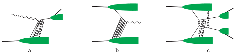
Figure 1: Graphs with gluon exchange between hadrons and the hard-scattering subprocess for semi-inclusive deep inelastic scattering (a), Drell-Yan production (b) and hadron pair production in $pp$ collisions (c).

Let us now return to the Wilson line in (1), which we have glossed over so far. When establishing factorization for processes such as Drell-Yan production or semi-inclusive deep inelastic scattering (SIDIS), one finds that an arbitrary number of gluons in a right-moving hadron can attach to the hard-scattering process without any twist suppression, provided that the gluons have polarization in the plus-direction. This is illustrated in Fig. 1a and b. It is the effect of these gluons that is summed up in the Wilson line $W(z_{2},z_{1})$, with a path between $z_{1}$ and $z_{2}$ that depends on the process.

For $\vec{k}$ integrated distributions, the situation simplifies if one works in the light-cone gauge $A^{+}=0$, where the Wilson line reduces to unity so that one has a literal parton model interpretation of the operator in (1) as creating and annihilating quarks or antiquarks. For $\vec{k}$ dependent distributions, however, there are subtle spin effects such as the Sivers or Boer-Mulders asymmetries, which are quite explicit in a covariant gauge, whereas in $A^{+}=0$ gauge they are due to Wilson line pieces at infinity, corresponding to gluon modes with $k^{+}=0$, see e.g. [7; 8].

Closer inspection shows that in TMDs one can actually not take the Wilson line $W(z_{2},z_{1})$ along a path in the light-like direction, since this leads to rapidity divergences [5]. To regulate these divergences, one can introduce a direction $v$ with nonzero plus- and minus-components, so that the resulting Wilson lines reduce to unity in the axial gauge $Av=0$ rather than in light-cone gauge. A formulation of factorization with TMDs in the framework of light-cone quantization and the $A^{+}=0$ gauge has so far not been achieved. On the positive side, the formulation with Wilson lines along a direction $v$ allows one to resum Sudakov logarithms to all orders. This has led to a successful phenomenology of processes with small measured transverse momentum, see [9; 10] and references therein. On a more fundamental level, the physical phenomena associated with TMDs force (and guide) us to think more deeply about the role of gluons and of gauge degrees of freedom when describing how parton emerge from hadrons and interact with each other.

Finally, we must note that TMD factorization has so far only been established for processes with a simple color structure in the hard scattering, such as SIDIS and Drell-Yan production. Serious obstacles for such a formulation have been identified for processes like the production of back-to-back hadrons or jets in $pp$ collisions, where graphs like the one in Fig. 1c do not appear to admit a resummation into Wilson line operators [11]. It remains an open question whether a factorized description (and along with it, Sudakov resummation with the same accuracy as for Drell-Yan production) can be found for this important class of processes.

2 Multiparton interactions: what are they and why are they interesting?

In a generic hadron-hadron collision, several partons in one hadron scatter on corresponding partons in the other hadron. At high energy, several of these scatters can have a hard scale and produce particles with large invariant mass or large transverse momenta. Examples are shown in Fig. 2. The effects of such multiparton interactions (also referred to as multiple interactions) average out or are power suppressed in sufficiently inclusive observables. This is why they are not included in the familiar factorization formulae for hadron-hadron collisions, which involve single-parton densities and a single hard-scattering subprocess. However, for more exclusive observables and more specific kinematics, contributions from multiple interactions can be substantial, and it has been estimated that they will play an important role in many analyses at the LHC. There is a long history of theoretical and experimental studies of such interactions, and the field has seen a strong boost in activity since the LHC has started operation, see e.g. the recent proceedings [12].

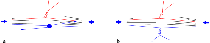
Figure 2: Double hard scattering processes producing a Drell-Yan lepton pair and a dijet (a) or two Drell-Yan pairs (b).

The description of multiparton interactions involves multiparton distributions, which are interesting in their own right since they contain information about correlations between different partons in the proton wave function. This information is inaccessible in the singe-parton distributions we discussed in Sect. 1.

The existing phenomenology of multiple interactions (including implementations in Monte Carlo event generators) is based on a simple and physically intuitive picture, which involves however many simplifying assumptions. A systematic treatment in QCD, which would match the level of sophistication achieved for single hard-scattering processes, remains to be given. Some steps into this direction have been taken in [13], and in the present proceedings we will point out results that have been obtained, open problems that have been identified, and prospects of using multiple interactions to learn more about hadron structure at the parton level and about theoretical approaches to understand this structure.

3 Some basic results

To begin with, let us specify the theoretical framework we will be using. We consider double hard scattering as the simplest (and often most prominent) case of multiparton interactions. Requiring both parton-level scattering processes to be hard allows us to use the concept of factorization and the predictive power of perturbation theory. Since the phenomenological interest in multiple interactions comes from the necessity to understand the hadronic final state in detail, we keep the transverse momenta of the produced particles differential and are hence led to using transverse-momentum dependent factorization and the associated multiparton distributions. Given the status of TMD factorization for single hard scattering described above, we consider the double Drell-Yan process of Fig. 2b as a case where the prospects for obtaining rigorous theory results are best, referring the practically important cases where secondary interactions produce jets to future work.

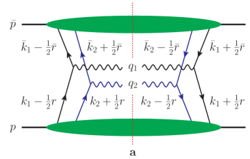
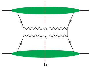
Figure 3: Graphs for the production of two electroweak gauge bosons by double (a) and by single (b) hard scattering. The dashed line indicates the final-state cut, and the decay of the bosons into leptons is not shown for simplicity.

The graph in Fig. 3a shows the production of a gauge boson pair by two hard-scattering processes. This graph can be evaluated with the same techniques that are used for single hard scattering, where small momentum components are neglected compared to large ones in each parton-level subprocess. In this approximation, the plus-momenta of right-moving partons and the minus-momenta of left-moving ones are fixed by the final-state kinematics, but their transverse momenta are not. With the momentum assignments in Fig. 3a, one finds $x_{i}=q_{i}^{+}/p^{+}$ and $\bar{x}_{i}=q_{i}^{-}/\bar{p}^{-}$ for the longitudinal parton momentum fractions. Momentum conservation gives $\vec{r}+\bar{\vec{r}}=\vec{0}$ for the transverse components of the momentum mismatch between partons on the left and the right of the final-state cut. The contribution of Fig. 3a to the cross section is then proportional to $\int d^{2}\vec{r}\,F_{a_{1},a_{2}}(x_{i},\vec{k}_{i},\vec{r})\,F_{\bar{a}_{1},\bar{a}_{2}}(\bar{x}_{i},\bar{\vec{k}}_{i},-\vec{r})$, where the first factor is the distribution for two quarks and the second factor the distribution for two antiquarks in the proton. Fourier transforming the distributions w.r.t. their last argument, one finds that the conjugate position variables satisfy $\bar{\vec{y}}=\vec{y}$, and the full expression of the cross section reads

$$\frac{d\sigma_{\,\text{Fig.~{}\ref{fig:double-single}a}}}{\prod_{i=1}^{2}dx_{i}\,d\bar{x}_{i}\,d^{2}\vec{q}{}_{i}} =\frac{1}{S}\sum_{\begin{subarray}{c}a_{1},a_{2}=q,\Delta q,\delta q\\[0.3014pt] \bar{a}_{1},\bar{a}_{2}=\bar{q},\Delta\bar{q},\delta\bar{q}\end{subarray}}\biggl{[}\,\prod_{i=1}^{2}\,\int d^{2}\vec{k}_{i}\,d^{2}\bar{\vec{k}}_{i}\;\delta^{(2)}(\vec{q}{}_{i}-\vec{k}_{i}-\bar{\vec{k}}_{i})\biggr{]}$$

$$\quad\times\hat{\sigma}_{1,a_{1}\bar{a}_{1}}(q_{1}^{2})\;\hat{\sigma}_{2,a_{2}\bar{a}_{2}}(q_{2}^{2})\int d^{2}\vec{y}\,F_{a_{1},a_{2}}(x_{i},\vec{k}_{i},\vec{y})\;F_{\bar{a}_{1},\bar{a}_{2}}(\bar{x}_{i},\bar{\vec{k}}_{i},\vec{y})\,,\phantom{\int}$$ (5)

where $\hat{\sigma}_{i,a_{i}\bar{a}_{i}}$ denotes the hard-scattering cross section for single-boson production. The statistical factor $S$ is $2$ if the produced bosons are identical and $1$ if they are not.

From our discussion in Sect. 1 it follows that the Fourier conjugate variable $\vec{y}$ of $\vec{r}$ represents the distance between the two scattering partons, averaged between the scattering amplitude and its complex conjugate. On the other hand, $\vec{k}_{1}$ and $\vec{k}_{2}$ are the transverse momenta of the partons, averaged in the same sense. $F_{a_{1},a_{2}}(x_{i},\vec{k}_{i},\vec{y})$ thus has the structure of a Wigner distribution in the transverse degrees of freedom. It is gratifying that this allows for a rather intuitive interpretation of the cross section formula (3): we have two quark-antiquark annihilation processes separated by a transverse distance $\vec{y}$, where in each annihilation the incident transverse parton momenta $\vec{k}_{i}$ and $\bar{\vec{k}}_{i}$ add up to the measured transverse momentum $\vec{q}_{i}$ of the produced gauge boson. Note, however, that the result (3) is fully quantum mechanical and has been obtained from Feynman graphs using standard approximations, without the need to appeal to semi-classical arguments. The operator definition of a two-quark distribution reads

$$F_{a_{1},a_{2}}(x_{i},\vec{k}_{i},\vec{y}) =\biggl{[}\,\prod_{i=1}^{2}\int\frac{dz_{i}^{-}d^{2}\vec{z}_{i}}{(2\pi)^{3}}\,e^{i(x_{i}z_{i}^{-}p^{+}-\vec{z}_{i}\vec{k}_{i})}\biggr{]}\;2p^{+}\!\!\!\int dy^{-}\big{\langle}p\,\big{|}\,\bar{q}(-\tfrac{1}{2}z_{2})\,W(-\tfrac{1}{2}z_{2},\tfrac{1}{2}z_{2})\,\Gamma_{a_{2}}\,q(\tfrac{1}{2}z_{2})\;$$

$$\quad\times\bar{q}(y-\tfrac{1}{2}z_{1})\,W(y-\tfrac{1}{2}z_{1},y+\tfrac{1}{2}z_{1})\,\Gamma_{a_{1}}\,q(y+\tfrac{1}{2}z_{1})\,\big{|}\,p\big{\rangle}\Big{|}_{z_{1}^{+}=z_{2}^{+}=y^{+}=0}$$ (6)

and is a natural extension of the definition of TMDs for a single parton described in Section 1.

The transverse-momentum integrated distribution $F_{a_{1},a_{2}}(x_{i},\vec{y})=\int d^{2}\vec{k}_{1}\,d^{2}\vec{k}_{2}\;F_{a_{1},a_{2}}(x_{i},\vec{k}_{i},\vec{y})$ gives the joint density of two quarks with momentum fractions $x_{1}$ and $x_{2}$ and relative transverse distance $\vec{y}$. It enters in the transverse-momentum integrated cross section as

$$\frac{d\sigma_{\,\text{Fig.~{}\ref{fig:double-single}a}}}{\prod_{i=1}^{2}dx_{i}\,d\bar{x}_{i}}=\frac{1}{S}\sum_{\begin{subarray}{c}a_{1},a_{2}=q,\Delta q,\delta q\\[0.3014pt] \bar{a}_{1},\bar{a}_{2}=\bar{q},\Delta\bar{q},\delta\bar{q}\end{subarray}}\hat{\sigma}_{1,a_{1}\bar{a}_{1}}(q_{1}^{2})\;\hat{\sigma}_{2,a_{2}\bar{a}_{2}}(q_{2}^{2})\int d^{2}\vec{y}\,F_{a_{1},a_{2}}(x_{i},\vec{y})\;F_{\bar{a}_{1},\bar{a}_{2}}(\bar{x}_{i},\vec{y})\,.$$ (7)

The integration over $\vec{k}_{1}$ and $\vec{k}_{2}$ puts the relative transverse coordinates $\vec{z}_{1}$ and $\vec{z}_{2}$ to zero in (3), so that in each quark-antiquark operator the two fields are separated by a light-like distance, as they are for the usual PDFs. However, the operators describing the first and the second quark are still separated by a transverse distance $\vec{y}$. The resulting distribution does therefore not involve a twist-four operator but rather the product of two operators with twist two.

For each of the two quark-antiquark operators there are three Dirac matrices $\Gamma_{a}$ that give a leading contribution to the cross section, namely $\Gamma_{q}=\tfrac{1}{2}\gamma^{+}$, $\Gamma_{\Delta q}=\tfrac{1}{2}\gamma^{+}\gamma_{5}$ and $\Gamma_{\delta q}^{j}=\tfrac{1}{2}i\sigma^{j+}\gamma_{5}$ with $j=1,2$. These matrices respectively project on unpolarized, longitudinally polarized and transversely polarized quarks and are well-known from the definition of single-parton densities. Note that for multiparton distributions one can have spin effects even in an unpolarized proton because the polarizations of different partons can be correlated among themselves. If such correlations are large, they leave an imprint in the cross section formulae (3) and (7), where they can change both the size of the cross section and the distribution of particles in the final state. In particular, one finds that a correlation between the transverse polarization of two quarks or antiquarks leads to an angular correlation between the leptonic decay planes of the two produced gauge bosons. Whether and where spin correlations between different partons in the proton are important is therefore an important question for phenomenology at the LHC. It is also of great interest from the point of view of hadron structure, and one may hope for a fruitful interplay between these two fields in the future.

Not only the spin but also the color of two partons can be correlated. In Eqs. (3) to (7) we have glossed over this degree of freedom, and it turns out that two-quark distributions can have two color structures, both of which contribute to the cross section. The two quark lines with momentum fraction $x_{1}$ in Fig. 3a can couple either to a color singlet or to a color octet. A corresponding color coupling of the two quark lines with momentum fraction $x_{2}$ then follows from color conservation. It is the color singlet combination that has the interpretation of a Wigner distribution discussed above, whereas the color octet combination describes an interference between different color states of a parton in the scattering amplitude and its complex conjugate. The operator defining the color octet combination reads $(\bar{q}_{2}\,\Gamma_{a_{2}}t^{a}q_{2})\,(\bar{q}_{1}\Gamma_{a_{1}}t^{a}q_{1})$, where $t^{a}$ denotes $\tfrac{1}{2}$ times the Gell-Mann matrices. The subscripts $1$ and $2$ of the quark fields indicate that after Fourier transformation the fields are associated with momentum fraction $x_{1}$ and $x_{2}$, respectively. Although the possibility of spin and color correlations in multiparton distributions has been pointed out long ago [14], the lack of a method to estimate their size has prevented them from being included in phenomenological analyses up to now.

In Sect. 1 we mentioned the resummation of Sudakov logarithms in single hard-scattering processes with small transverse momenta. Such logarithms also appear in the double scattering process depicted in Fig. 3a. They can be computed by generalizing the method of [15; 16] from single to double hard scattering. An important result is that the leading double logarithms in $\vec{q}_{i}^{2}/Q^{2}$ are given by the product of the corresponding factors for each separate hard-scattering process. Beyond this accuracy, the structure becomes more involved since soft gluons can be exchanged between all parton lines in Fig. 3a. Explicit calculation shows that these effects also lead to a mixing between the color singlet and color octet distributions mentioned in the previous paragraph.

4 Power counting: when are multiple interactions suppressed and when are they not?

When deriving the cross section formula (3) we have taken the leading approximation in the small parameter $\Lambda/Q$, where the large scale is provided by $Q^{2}\sim q_{1}^{2}\sim q_{2}^{2}$, whereas the small scale $\Lambda$ is given by the transverse boson momenta $|\vec{q}_{1}|$, $|\vec{q}_{2}|$ or by the scale of nonperturbative interactions, whichever is larger. One readily finds that, up to logarithmic terms, the overall scaling behavior of the double-scattering cross section (3) is

$$\frac{d\sigma_{\,\text{Fig.~{}\ref{fig:double-single}a}}}{\prod_{i=1}^{2}dx_{i}\,d\bar{x}_{i}\;d^{2}\vec{q}_{i}} \sim\,\frac{1}{Q^{4}\Lambda^{2}}\,.$$ (8)

One finds the same behavior for the case where the two bosons are produced in a single hard scattering, as illustrated in Fig. 3b. In the fully differential cross section, multiple hard interactions are thus not power suppressed with single hard scattering and can hence be of significant size.

The situation changes if one integrates over the transverse momenta $\vec{q}_{1}$ and $\vec{q}_{2}$. In the double scattering mechanism both $|\vec{q}_{1}|$ and $|\vec{q}_{2}|$ result from transverse parton momenta and are hence limited to size $\Lambda$. By contrast, with a single hard scattering the sum $|\vec{q}_{1}+\vec{q}_{2}|$ is of order $\Lambda$ but the individual transverse momenta can be as large as kinematically allowed, i.e. they can be of order $Q$. Single hard scattering can thus populate a larger phase space, and one has

$$\frac{d\sigma_{\,\text{Fig.~{}\ref{fig:double-single}a}}}{\prod_{i=1}^{2}dx_{i}\,d\bar{x}_{i}} \sim\,\frac{\Lambda^{2}}{Q^{4}}\,, \frac{d\sigma_{\,\text{Fig.~{}\ref{fig:double-single}b}}}{\prod_{i=1}^{2}dx_{i}\,d\bar{x}_{i}} \sim\,\frac{1}{Q^{2}}\,.$$ (9)

The double scattering contribution is now power suppressed in the overall cross section. This is indeed necessary for the consistency of the usual factorization formulae, which only describe the single scattering contribution.

Multiple interactions are thus important in observables that are sufficiently exclusive and in kinematics where this mechanism can contribute. The relevant kinematic regions are those where one has subsets of final-state particles for which the vector sum of transverse momenta is small compared with the hard scale in the process. In our case this is the double Drell-Yan process with small transverse momenta of the produced vector bosons. Another important example emphasized in [17] is the production of two dijet pairs, each of which is approximately back-to-back.

5 High transverse momentum

The predictive power of the theory increases if one considers kinematics where the transverse momenta $\vec{q}_{i}$ are large compared with the scale of nonperturbative interactions (while still being small compared with the very large scale $Q$). At least some of the transverse parton momenta are then large as well, and one can compute the transverse-momentum dependent multiparton distributions in terms of a perturbative subprocess at scale $|\vec{q}_{i}|$ and distributions that depend on fewer variables.

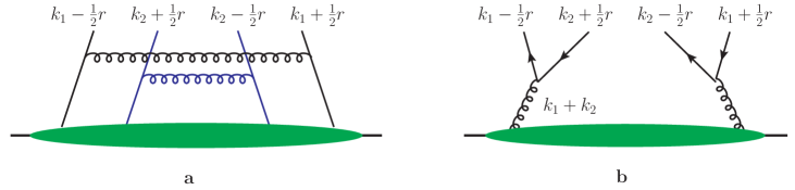
Figure 4: Graphs where partons with high transverse momentum are generated by parton radiation (a) or by the splitting of a single parton into two (b).

Two types of graphs are of particular importance in this context. In the double ladder graph of Fig. 4a, each of the two partons that will enter the collision process acquires a large transverse momentum by radiating a parton into the final state. This is a straightforward generalization of the corresponding mechanism for single-parton densities at large $\vec{k}$. The two ladders in the graph are independent, so that this mechanism can contribute for interparton distances $\vec{y}$ of hadronic size. An important finding is that the color factors for ladder graphs favor the case where the parton pairs with equal momentum fraction $x_{1}$ or $x_{2}$ are coupled to color singlets. It remains to be studied quantitatively how strong this preference for the color singlet channel is.

In the graph of Fig. 4a a single parton splits into two partons with high transverse momenta, both of which will then take part in a hard collision process. This mechanism is in particular relevant for large $\vec{r}$, which translates to a small distance $\vec{y}$. One finds that the transverse-momentum integrated distribution $F(x_{i},\vec{y})$ behaves like $1/\vec{y}^{2}$ at small $\vec{y}$ due to these splitting graphs. This poses a problem of consistency, since the integral over $\vec{y}$ in the cross section (7) is then linearly divergent in $\vec{y}^{2}$ at short distances. Likewise, one finds that the $\vec{y}$ integral in (3) diverges logarithmically at small $\vec{y}$. The underlying problem signaled by these divergences is that the graph shown in Fig. 5 can be interpreted in two ways. If one identifies the two boxes in the figure as representing the splitting graphs for a quark-antiquark distribution, one has a graph for double hard scattering as just discussed. However, without the boxes one has a graph for single hard scattering, namely for the fusion of two gluons into two electroweak gauge bosons via a quark loop. For a detailed investigation of this loop graph we refer to [18]. A proper theoretical formulation will need to make sure that there is no double counting problem for this graph and remove the divergences in the $\vec{y}$ integration of the double scattering cross sections (3) and (7). To achieve this in a consistent and practicable way is an outstanding problem.

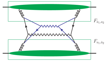
Figure 5: Graph for the production of two gauge bosons, where in both colliding protons an initial gluon splits into a quark-antiquark pair. The boxes indicate the splitting graph of Fig. 4b for a quark-antiquark distribution.

6 Approximation by single-parton distributions

To develop a phenomenology of multiple interactions, one needs a simple ansatz for multiparton distributions as a starting point. For those distributions that admit an interpretation as Wigner distributions it is natural to approximate them by the product of single-parton densities, neglecting any possible correlations between the different partons.

To formalize such an ansatz we insert a complete set of intermediate states $\sum_{X}|X\rangle\langle X|$ between the two operators $(\bar{q}_{2}\,\Gamma_{a_{2}}q_{2})$ and $(\bar{q}_{1}\,\Gamma_{a_{1}}q_{1})$ in the definition (3) of the two-parton distribution. If we assume that this sum is dominated by single-proton states, then we obtain an approximation in terms of single-parton distributions. For transverse-momentum integrated distributions, this approximation reads

$$F_{a_{1},a_{2}}(x_{i},\vec{y}) \approx\int d^{2}\vec{b}\;f_{a_{2}}(x_{2},\vec{b})\,f_{a_{1}}(x_{1},\vec{b}+\vec{y})\,,$$ (10)

where $f_{a}(x,\vec{b})$ is the impact parameter distribution of parton $a$ discussed in Sect. 1. This approximation, visualized in Fig. 6, is the starting point of most estimates for multiparton scattering in the literature, although there is a number of attempts to go beyond it [19; 20; 21].

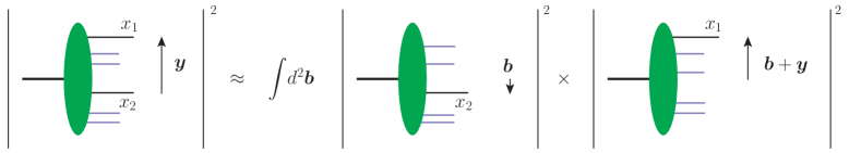
Figure 6: Visualization of the approximation (10) of a two-parton distribution in terms of impact parameter densities for single partons. In the figure we use that both types of distributions can be represented as squares of light-cone wave functions of the proton.

The corresponding approximation for transverse-momentum dependent distributions has a simpler structure if we use the variable $\vec{r}$ rather than $\vec{y}$. We then have

$$F_{a_{1},a_{2}}(x_{i},\vec{k}_{i},\vec{r}) \approx f_{a_{2}}(x_{2},\vec{k}_{2}-\tfrac{1}{2}x_{2}\vec{r};-\vec{r})\,f_{a_{1}}(x_{1},\vec{k}_{1}-\tfrac{1}{2}x_{1}\vec{r};\vec{r})\,.$$ (11)

Here $f_{a}(x,\vec{k},\vec{r})$ is a transverse-momentum dependent generalized parton distribution, defined by the Fourier transform of a matrix element as in (1), where the annihilated quark carries momentum fraction $x$ and transverse momentum $\vec{k}-\tfrac{1}{2}\vec{r}$ and the created quark carries momentum fraction $x$ and transverse momentum $\smash{\vec{k}+\tfrac{1}{2}\vec{r}}$.

This strategy of approximation can also be adapted to the color octet distributions described in Sect. 3, which cannot be interpreted as Wigner distributions. To this end, we perform a Fierz transformation in color and in spin space,

$$(\bar{q}_{2}\,\Gamma_{a_{2}}t^{a}q_{2})\,(\bar{q}_{1}\Gamma_{a_{1}}t^{a}q_{1}) =-\tfrac{1}{6}\,(\bar{q}_{2}\,\Gamma_{a_{2}}q_{2})\,(\bar{q}_{1}\Gamma_{a_{1}}q_{1})+\tfrac{1}{2}\sum_{b_{1},b_{2}}c_{a_{1}a_{2},b_{1}b_{2}}\,(\bar{q}_{1}\Gamma_{b_{2}}\,q_{2})\,(\bar{q}_{2}\,\Gamma_{b_{1}}\,q_{1})\,,$$ (12)

where the coefficients $c_{a_{1}a_{2},b_{1}b_{2}}$ are straightforward to calculate. The first term on the r.h.s. is a color singlet distribution and can be approximated as described above. In the second term, the quark and antiquark fields coupled to color singlets are now associated with different longitudinal momentum fractions. Repeating the steps that lead to (11) one finds that this term is represented by transverse-momentum dependent GPDs in which not only the transverse but also the longitudinal parton momenta differ between the created and the annihilated quark. This just means that the skewness variable $\xi$ mentioned in Sect. 1 is nonzero in this case.

It should be emphasized that the above approximations are ad hoc in the sense that we cannot quantify to which extent the sum over all intermediate states $X$ in our derivation is actually dominated by single-proton states. However these approximations may serve as a starting point, and they can give valuable information about aspects that are poorly known otherwise, such as the distribution of partons in transverse space and the possible size of color interference effects.

7 Possible strategies for modeling multiparton distributions

Our current knowledge of multiparton distributions is very limited, and it should be interesting to investigate them in approaches that have successfully been applied to single-parton densities. The comparison of predictions obtained in such approaches with upcoming data on multiple interactions at LHC could lead to significant progress, with benefits for both sides.

One possible avenue is to take Mellin moments of two-parton distributions and to study the resulting matrix elements in lattice QCD as described in [13]. This will naturally give limited information about the dependence of the distributions on their momentum fractions $x_{i}$, but it has the potential to quantify parton correlations in a genuinely nonperturbative framework.

Constituent quark models, chiral quark models, the Dyson-Schwinger approach and similar methods should be suitable to evaluate not only the distributions of single partons but also two-parton distributions. As illustrated by simple examples in [13], one may expect two-parton correlations of significant size in these approaches. They can also be used to investigate the degree of validity of the approximations (10) and (11).

The two avenues just discussed will mostly give information about partons with momentum fractions $x_{i}$ above, say, $0.1$. In multiple interactions at LHC, typical values of $x_{i}$ are smaller by at least an order of magnitude. One way to investigate this region would be to take the results from quark models as an input for scale evolution, which will generate partons with lower $x_{i}$ by perturbative splitting as the scale is increased. Obvious questions to study in this context are to which extent scale evolution may wash out two-parton correlations present at low scales, and whether evolution to higher scales might improve the quality of the approximation in (10). These would be important lessons, even if one has to bear in mind that perturbative evolution alone cannot account for sea quarks and gluons at small $x$, as already mentioned in the beginning of Sect. 1. An outstanding challenge for the study of hadron structure is to find and develop nonperturbative approaches suitable to describe these degrees of freedom in a quantitative way.

- [1] Glück, M., Reya, E., Vogt, A.: Dynamical parton distributions revisited, Eur. Phys. J. C5, 461 (1998) [hep-ph/9806404].
- [2] Jimenez-Delgado, P., Reya, E.: Dynamical NNLO parton distributions, Phys. Rev. D79, 074023 (2009) [arXiv:0810.4274].
- [3] Burkardt, M.: Impact parameter space interpretation for generalized parton distributions, Int. J. Mod. Phys. A18, 173 (2003) [hep-ph/0207047].
- [4] Hägler, Ph.: Hadron structure from lattice quantum chromodynamics, Phys. Rept. 490, 49 (2010) [arXiv:0912.5483].
- [5] Collins, J. C.: Rapidity divergences and valid definitions of parton densities, PoS LC2008, 028 (2008) [arXiv:0808.2665].
- [6] Hillery, M., O’Connell, R. F., Scully, M. O., Wigner, E. P.: Distribution Functions in Physics: Fundamentals, Phys. Rept. 106, 121 (1984).
- [7] Collins, J. C.: Leading twist single transverse-spin asymmetries: Drell-Yan and deep inelastic scattering, Phys. Lett. B536, 43 (2002) [hep-ph/0204004].
- [8] Belitsky, A. V., Ji, X., Yuan, F.: Final state interactions and gauge invariant parton distributions, Nucl. Phys. B656, 165 (2003) [hep-ph/0208038].
- [9] Nadolsky, P. M.: Multiple parton radiation in hadroproduction at lepton hadron colliders, [hep-ph/0108099].
- [10] Aybat, S. M., Rogers, T. C.: TMD Parton Distribution and Fragmentation Functions with QCD Evolution, Phys. Rev. D83, 114042 (2011) [arXiv:1101.5057].
- [11] Rogers, T. C., Mulders, P. J.: No Generalized TMD-Factorization in Hadro-Production of High Transverse Momentum Hadrons, Phys. Rev. D81, 094006 (2010) [arXiv:1001.2977].
- [12] Bartalini, P. et al.: Multiple partonic interactions at the LHC. Proceedings of MPI 08, Perugia, Italy, October 27–31, 2008, [arXiv:1003.4220].
- [13] Diehl, M., Schäfer, A.: Theoretical considerations on multiparton interactions in QCD, Phys. Lett. B698, 389 (2011) [arXiv:1102.3081].
- [14] Mekhfi, M.: Correlations In Color And Spin In Multiparton Processes, Phys. Rev. D32, 2380 (1985).
- [15] Collins, J. C., Soper, D. E.: Back-To-Back Jets in QCD, Nucl. Phys. B193, 381 (1981).
- [16] Collins, J. C., Soper, D. E., Sterman, G. F.: Transverse Momentum Distribution in Drell-Yan Pair and and Boson Production, Nucl. Phys. B250, 199 (1985).
- [17] Blok, B., Dokshitser, Yu., Frankfurt, L., Strikman, M.: pQCD physics of multiparton interactions, [arXiv:1106.5533].
- [18] Gaunt, J. R., Stirling, W. J.: Double Parton Scattering Singularity in One-Loop Integrals, JHEP 1106, 048 (2011) [arXiv:1103.1888].
- [19] Calucci, G., Treleani, D.: Proton structure in transverse space and the effective cross-section, Phys. Rev. D60, 054023 (1999) [hep-ph/9902479].
- [20] Domdey, S., Pirner, H. J., Wiedemann, U. A.: Testing the Scale Dependence of the Scale Factor in Double Dijet Production at the LHC, Eur. Phys. J. C65, 153 (2010) [arXiv:0906.4335].
- [21] Rogers, T. C., Strikman, M.: Multiple Hard Partonic Collisions with Correlations in Proton-Proton Scattering, Phys. Rev. D81, 016013 (2010) [arXiv:0908.0251].