Transfer and scattering of wave packets by a nonlinear trap

Abstract

In the framework of a one-dimensional model with a tightly localized self-attractive nonlinearity, we study the formation and transfer (dragging) of a trapped mode by “nonlinear tweezers”, as well as the scattering of coherent linear wave packets on the stationary localized nonlinearity. The use of the nonlinear trap for the dragging allows one to pick up and transfer the relevant structures without grabbing surrounding “garbage”. A stability border for the dragged modes is identified by means of of analytical estimates and systematic simulations. In the framework of the scattering problem, the shares of trapped, reflected, and transmitted wave fields are found. Quasi-Airy stationary modes with a divergent norm, that may be dragged by the nonlinear trap moving at a constant acceleration, are briefly considered too.

I Introduction

Solitons, in the form of robust localized pulses propagating in nonlinear dispersive media, have been studied extensively in various physical contexts dau . Many works have been dealing with the soliton dynamics in media featuring uniform nonlinearities, modeled by wave equations with constant nonlinearity coefficients. More recently, much attention has been drawn to the study of solitons in structured media, which feature spatial modulations of the local nonlinearity strength (see recent review Barcelona ), including the case when stable bright solitons may be supported by self-defocusing nonlinearity whose strength grows towards the periphery Barcelona2 . In solid-state physics, effective potentials induced by the nonlinearity modulation are often called pseudopotentials Harrison . Recently developed experimental techniques make it possible to realize such structures in photonics and Bose-Einstein condensates (BECs). Particularly, in photonic media, the modulation profiles can be induced by nonuniform distributions of resonant dopants affecting the local nonlinearity, which may be created by means of in-diffusion technology technology . Another possibility is to use photonic crystals with voids infiltrated by liquids, which are matched to the host material in terms of the refractive index, but feature a mismatch in the Kerr coefficient infiltration . On the other hand, in the context of BECs, the local nonlinearity can be spatially modulated by means of the Feshbach resonance, induced by nonuniform magnetic Inouye or electric Marinescu fields, as well as by an appropriate optical field Fedichev .

One-dimensional (1D) solitons were studied theoretically in the context of pseudopotential structures in BECs BECpseudopotential ; Nir and optics Hao ; Barcelona2 . The possible use of 1D nonlinearity-modulation profiles was also elaborated in models of matter-wave lasers, designed so as to release periodic arrays of coherent pulses laser ; Humberto (although the first experimentally realized prototypes of atomic-wave lasers were built in a different way real-laser ). Self-focusing pseudopotentials were theoretically studied in the two-dimensional (2D) geometry too, demonstrating that it is much more difficult (but possible) to stabilize 2D solitons in such settings, than using familiar linear potentials or lattices Sakaguchi2 ; Fibich ; JMO , while the above-mentioned self-defocusing structures solves this problem easily Barcelona2 .

The simplest example of the pseudopotential corresponds to the nonlinearity concentrated at a single point, which is accounted for by the $\delta$-function Azbel . In optics, it may represent a planar waveguide with a narrow nonlinear stripe embedded into it (stable spatial solitons supported by narrow stripes carrying the quadratic, rather than cubic, nonlinearity were found in Refs. Canberra ; Asia ). In BECs, the localized nonlinearity may be imposed by a tightly focused laser beam inducing the Feshbach resonance. A relevant extension of such a nonlinear spot is the model of the double-well pseudopotential; in the simplest form, it is based on a symmetric set of two $\delta$-functions multiplying the cubic term in the respective nonlinear Schrödinger (NLS) equation DeltaSSB , or the quadratic nonlinearity in the model of the second-harmonic generation Asia . In either case, full analytical solutions have been found for symmetric, asymmetric and antisymmetric localized modes trapped by the set of the two $\delta$-functions. In addition to that, full symmetric and asymmetric solutions can be found Valera for a similar discrete model, with two cubic-nonlinear sites embedded into a linear host chain, which was introduced (without the consideration of the spontaneous symmetry breaking) in Refs. Tsironis . The symmetry-breaking problem was also recently analyzed in the two-dimensional setting, for a symmetric pair of nonlinear circles embedded into a linear host medium JMO .

The model with the single nonlinear $\delta$-function readily gives rise to a family of exact soliton solutions—see Eq. (5) below—which are completely unstable, but may be stabilized if the point-like nonlinearity is combined with a periodic linear potential (in the same setting, the localized nonlinearity with the repulsive sign may support stable gap solitons) Nir . In the present work, we demonstrate that nonlinear self-trapped states may also be stabilized, without adding any linear potential, by the regularized localized nonlinearity, if the ideal $\delta$-function is replaced by a Gaussian profile.

In addition to supporting stationary trapped modes, the localized potentials may be used as tweezers, for the transfer of the trapped modes, which is a topic with many potential applications we . In particular, the use of the $\delta$-functional linear trapping potentials makes it possible to find exact solutions for various transfer problems Edik ; Adolfo . The dynamical process of extracting matter-wave pulses from a BEC reservoir by nonlinear tweezers, induced by an appropriate laser beam, was simulated in detail in Ref. Humberto .

The main objective of the present work is to analyze possibilities of the controlled transfer of localized wave packets by a moving nonlinear trapping pseudopotential (nonlinear tweezers), represented by a narrow Gaussian profile multiplying the self-focusing cubic nonlinearity. An advantage of using the nonlinear tweezers is that they would not grab and drag small-amplitude (radiation) “garbage”, surrounding the target object in a realistic setting, and one may use the amplitude of the object to control its transfer (this resembles the well-known advantage of nonlinear optical amplifiers in comparison with their linear counterparts—see Ref. nonlin and references therein). The model is introduced in Section 2, where we also produce simple analytical results for the transfer problem, obtained by means of the adiabatic approximation, which is appropriate for a slowly moving trap. Basic numerical results are reported in Section 3. We also briefly consider a related problem of dragging wave patterns with a divergent norm by the nonlinear trap moving at a constant acceleration, which is relevant in connection to the recently considered transmission regimes for Airy beams, exact Berry or approximate Airy , including their nonlinear generalizations Airy-nonlinear , and the transfer of linear trapped wave packets by a potential well moving at a constant acceleration Er'el . In Section 4, we report results for another natural problem related to the present setting, namely, the scattering of linear wave packets on the localized stationary attractive nonlinearity. Section 5 concludes the paper.

II The model and adiabatic approximation

II.1 The formulation

The model with the tightly localized nonlinear trap, which represents the moving tweezers, is based on the following normalized version of the NLS equation for wave function $\psi(x,t)$:

$$i\psi_{t}=-\frac{1}{2}\psi_{xx}-\tilde{\delta}\left(x-\xi(t)\right)\left|\psi\right|^{2}\psi,$$ (1)

where subscripts denote partial derivatives, while $\tilde{\delta}(x)$ and $\xi(t)$ define the shape of the nonlinear trap and its law of motion. In the context of BECs, Eq. (1) is a normalized version of the Gross-Pitaevskii equation, with time $t$ and coordinate $x$ [note that in an early work Azbel , Eq. (1) was introduced as a model for tunneling of attractively interacting particles through a junction]. In the optical model, $t$ is replaced by the propagation distance ($z$), while $x$ is the transverse coordinate in the respective planar waveguide.

In the first version of the model, the nonlinear trap was taken in the form of the ideal delta-function, $\tilde{\delta}\left(x\right)=\delta(x)$ Azbel . In the present work, numerical results are reported for its practically relevant Gaussian regularization, namely

$$\tilde{\delta}(x)=\left(2\sqrt{\pi\epsilon}\right)^{-1}\exp\left(-x^{2}/\left(4\epsilon\right)\right),$$ (2)

with a sufficiently small width $\epsilon$. The law of motion for the moving trap will be taken as

$$\xi(t)=\left\{\begin{array}[]{cc}0,&\mathrm{at~{}}~{}t\leq 0,\\ \frac{1}{2}\Xi\left[1+\sin\left(\pi\frac{t-T/2}{T}\right)\right],&\mathrm{at~{}}~{}0<t<T,\\ \Xi&\mathrm{at~{}}~{}t\geq T,\end{array}\right.$$ (3)

which implies that the trap is smoothly transferred from the initial position, $\xi=0$, starting at $t=0$, to the final position, $\xi=\Xi$, at $t=T$. Both the initial and final velocities corresponding to this law of motion are zero, i.e., $d\xi/dt(t=0)=d\xi/dt(t=T)=0$.

II.2 Pulse solutions

The model with the quiescent trap ($\xi=0$), described by the ideal $\delta$-function, allows one to construct solutions to Eq. (1) as a combination of two solutions of the linear Schrödinger equation in free space at $x<0$ and $x>0$, coupled by the derivative-jump condition at $x=0$ (while the wave function itself must be continuous at this point):

$$\psi_{x}(x=+0)-\psi_{x}\left(x=-0\right)=-2\left|\psi(x=0)\right|^{2}\psi(x=0).$$ (4)

This condition gives rise to a family of obvious solutions to Eq. (1) with $\tilde{\delta}(x)=\delta(x)$ and $\xi=0$:

$$\psi=\left(-2\mu\right)^{1/4}e^{-i\mu t}e^{-\sqrt{-2\mu}|x|},$$ (5)

where $\mu<0$ is an arbitrary chemical potential. Such soliton-like solutions, with a discontinuous first derivative, are usually called peakons (see, e.g., Refs. camholm ). Note that the norm of the peakon family does not depend on the chemical potential, namely,

$$N\equiv\int_{-\infty}^{+\infty}\left|\psi(x)\right|^{2}dx=1.$$ (6)

This degeneracy resembles the well-known feature of the Townes solitons in the two-dimensional NLS equation with the uniform nonlinearity Berge . Accordingly, the application of the Vakhitov-Kolokolov (VK) stability criterion, $dN/d\mu<0$ VK ; Berge , formally predicts the neutral stability of the peakon family; nevertheless, a numerical study demonstrates that the entire family is unstable Nir , the instability being similar to that of the Townes solitons in two dimensions Berge . As mentioned above, the peakons can be stabilized by the addition of the linear periodic potential (with the nonlinear $\delta$-function placed at an arbitrary position with respect to the potential Nir ). In the next section, we demonstrate that stabilization may also be induced by the regularization of the $\delta$-function, as per Eq. (2). Generally speaking, it is easy to stabilize the family of Townes-like solitons, because the linearization of the underlying equation with respect to small perturbations around the soliton does not give rise to any unstable eigenvalue; in fact, the instability is nonlinear, i.e., it grows not exponentially, but rather as a power of time, and is represented by a respective pair of zero eigenvalues. Therefore, any modification of the equation which shifts the zero eigenvalues in the direction of real frequencies may stabilize the entire family. This will be the case in our considerations below (in Section 3) with the finite-width Gaussian (2) replacing the $\delta$-function.

Assuming that a stabilization mechanism is in action, but the shape of the soliton does not substantially deviate from Eq. (5), it is natural to expect that the trap, slowly moving according to given $\xi(t)$ [see, e.g., Eq. (3)], may drag the trapped soliton, which will then be described by the following modification of solution (5), in the adiabatic approximation:

$$\psi=\left(-2\mu\right)^{1/4}\exp\left[-i\mu t+\frac{i}{2}\int\left(\frac{d\xi}{dt}\right)^{2}dt+i\frac{d\xi}{dt}x\right]\exp\left[-\sqrt{-2\mu}\left|x-\xi(t)\right|\right].$$ (7)

In fact, expression (7) is the usually defined Galilean boost of peakon (5) moving at instantaneous velocity $d\xi/dt$.

II.3 Airy waves

For the consideration of the nonlinear trap moving with constant acceleration $W$, we set $\xi(t)=\left(W/2\right)t^{2}.$ Then, Eq. (1) can be rewritten in the accelerating reference frame moving along with the trap, i.e., in terms of the following variables:

$$\psi\left(x,t\right) \equiv \left(W/4\right)^{1/6}\phi\left(z,\tau\right)\exp\left[iWt\left(x-Wt^{2}/3\right)\right],$$ (8)

$$z \equiv \left(2W\right)^{1/3}\left(x-Wt^{2}/2\right),\quad\tau\equiv\left(W^{2}/2\right)^{1/3}t.$$ (9)

The accordingly transformed Eq. (1) reads:

$$i\phi_{\tau}+\phi_{zz}-z\phi+\delta\left(z-z_{0}\right)\left|\phi\right|^{2}\phi=0,$$ (10)

where $z_{0}$ is the location of the nonlinear trap with respect to the accelerating reference frame. Stationary solutions to Eq. (10) are $\phi(z,\tau)\equiv a(z)$, with real function $a(z)$ obeying the following equation:

$$\frac{d^{2}a}{dz^{2}}-za+\delta\left(z-z_{0}\right)a^{3}=0.$$ (11)

Without the nonlinear term, Eq. (11) is the classical Airy equation, whose relevant solutions at $z<z_{0}$ and $z>z_{0}$ are, respectively, given by:

$$a_{-}(z)=C_{1}\mathrm{Ai}(z)+C_{2}\mathrm{Bi}(z),~{}a_{+}(z)=C_{3}\mathrm{Ai}(z).$$ (12)

Here, $C_{1}$ and $C_{2}$ are constants, and $\mathrm{Ai}(z)$, $\mathrm{Bi}(z)$ are the standard Airy functions which are defined by their asymptotic forms at $z\rightarrow-\infty$ and $z\rightarrow+\infty$ Abram :

$$\left\{\mathrm{Ai,Bi}\right\}(z)\approx\frac{1}{\sqrt{\pi}\left(-z\right)^{1/4}}\left\{\sin,\cos\right\}\left(\frac{\pi}{4}+\frac{2}{3}\left(-z\right)^{3/2}\right),$$ (13)

$$\left\{\mathrm{Ai,Bi}\right\}(z)\approx\frac{1}{2\sqrt{\pi}z^{1/4}}\exp\left(\mp\frac{2}{3}z^{3/2}\right)~{}.$$ (14)

Using the Wronskian of the Airy functions, which is equal to $1/\pi$ Abram , the continuity condition for $\phi(z)$ and jump relation (4) at $z=z_{0}$ give coefficients $C_{1,2,3}$ [see Eq. (12)] in terms of the amplitude of the solution, $A\equiv a(z=z_{0})$, and $z_{0}$ itself, that may be considered as two free parameters of the solution family:

$$C_{1} = \left[\left(\mathrm{Ai}(z_{0})\right)^{-1}-\pi\mathrm{Bi}(z_{0})A^{2}\right]A,$$

$$C_{2} = \pi\mathrm{Ai}(z_{0})A^{3},$$

$$C_{3} = A\left(\mathrm{Ai}(z_{0})\right)^{-1}.$$ (15)

The known peculiarity of solutions based on the Airy functions is the divergence of the norm in the tail at $z\rightarrow-\infty$, as the corresponding average density produced by Eqs. (12) and (13),

$$\left\langle a^{2}(z)\right\rangle\approx\frac{C_{1}^{2}+C_{2}^{2}}{2\pi\sqrt{-z}},$$ (16)

decays too slowly. In time-dependent settings, the divergence of the norm implies a gradual decay of the initial pulse, which loses its power sucked into the tail growing toward $z\rightarrow-\infty$ Airy .

III Numerical results for the transfer and dragging problems

III.1 Stability conditions for the transfer

First, we have constructed a family of stationary solutions to Eq. (1) with the quiescent ($\xi=0$) regularized nonlinearity profile, taken as per Eq. (2), in the form of $\psi(x,t)=e^{-i\mu t}w(x)$, where the real function $w(x)$ satisfies the equation:

$$\mu w=-\frac{1}{2}\frac{d^{2}w}{dx^{2}}-\tilde{\delta}(x)w^{3}.$$ (17)

A typical example of the solution is displayed in Fig. 1(a), and the entire family of solutions is represented in Fig. 1(b) by the corresponding $N(\mu)$ curve, cf. the degenerate dependence given by Eq. (6) for the ideal $\delta$-function. It is obvious that the entire family satisfies the VK criterion, $dN/d\mu<0$, hence the solitons may be stable. This conjecture has been verified through the computation of the stability eigenvalues for perturbations around the steady-state solution of Eq. (17), and also by means of direct simulations of the perturbed evolution (not shown here). All the eigenvalues were found to be purely imaginary (they are defined so that imaginary values correspond to the real frequencies, i.e., neutral stability), therefore only the edge of the (continuous) spectrum lying on the imaginary axis is shown in Fig. 1(c). This stabilization is a direct result of the regularization of the $\delta$-function in Eq. (17). We have checked that, as smaller values of the regularization parameter, $\epsilon$, are taken, the corresponding stationary wave function $w$ approaches the peakon profile of Eq. (5). It is worthy to note that, as the limit of the ideal $\delta$-function is approached, we observe a pair of eigenvalues that bifurcate from the edge of the continuous spectrum and approach the origin, where they formally arrive in the limit of $\epsilon\rightarrow 0$, at which point the scaling invariance associated with Eq. (6) is restored, and the nonlinear instability emerges.

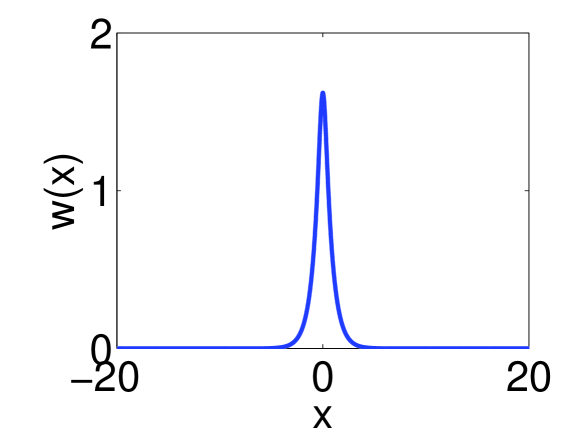
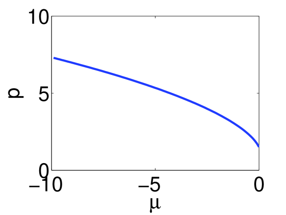
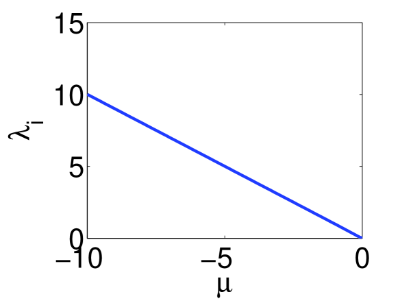
Figure 1: (Color online) (a) An example of a numerically found stationary solution of Eq. (17) with $\mu=-1$ and $\tilde{\delta}(x)$ taken per Eq. (2). (b) The norm of the solutions, defined according to Eq. (6), vs. chemical potential $\mu$. (c) The edge of the continuous spectrum lying on the imaginary axis [the full eigenvalue is defined as $i\lambda_{\mathrm{i}}$, the continuous spectrum occupying the area above the border shown in (c)]. These results are obtained for a width of the moving trap of $\epsilon=0.05$.

We now turn to characteristic examples (cf. Fig. 2) of the transfer of originally stable quiescent solitons by the nonlinear trap moving according to Eq. (3). As might be expected, the soliton survives the transfer, provided that it is not dragged too hard, i.e., the transfer time, $T$, is not too short. We define the soliton as “surviving the transfer” if, at time $t=T$, its amplitude is no smaller than a sufficiently high fraction of the initial soliton amplitude—say, $90\%$ or $80\%$. For instance, in the case shown in Fig. 2, the soliton dragged by the trap of width $\epsilon=0.05$ keeps $90\%$ of the initial amplitude for $T\geq 20$. It can be checked that, in all cases of the “survival”, the motion of the dragged soliton accurately follows the prediction of the adiabatic approximation [Eq. (7)], as is clearly seen in the example displayed in Fig. 2(c), where the actual trajectory of the dragged mode closely follows the adiabatic trajectory $\xi(t)$. The surviving solitons essentially preserve their original shape of the smoothed peakon, cf. Figs. 1(a) and 2(d,e,f). The three latter figures demonstrate that the eventual shape of the transferred mode is nearly the same for three different values of the trap’s width, $\epsilon=0.05$, $0.1$, and $0.025$, i.e., the eventual results are robust, withstanding the variation of essential parameters of the scheme within wide limits.

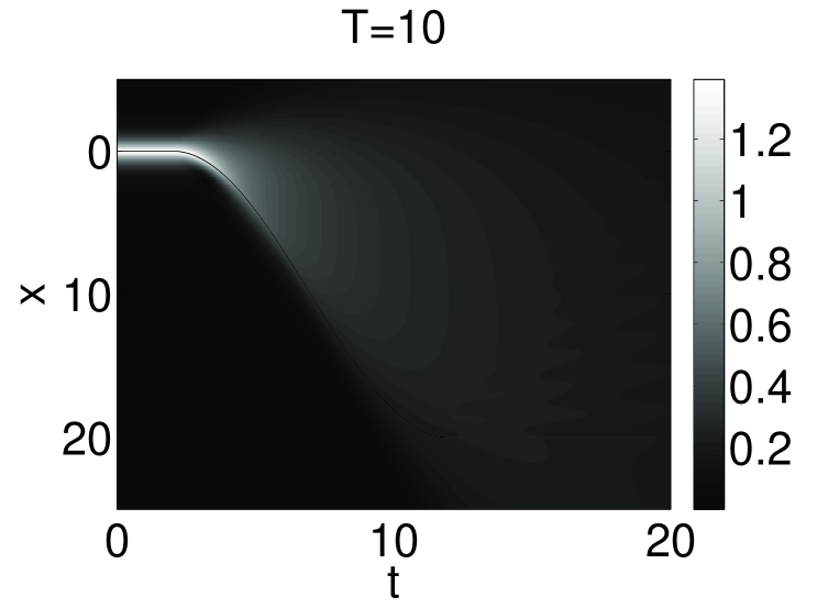
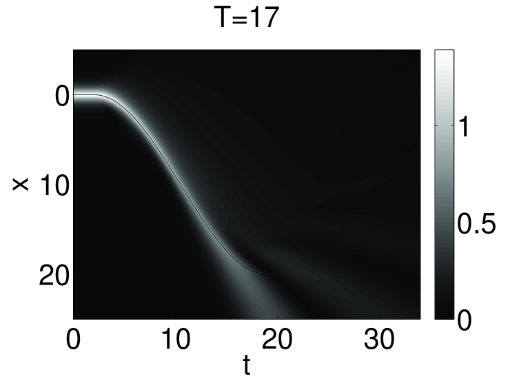
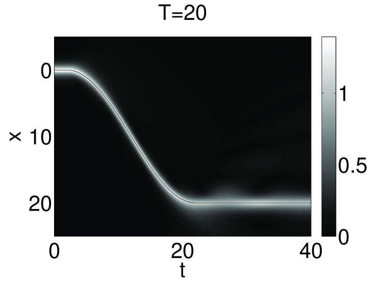
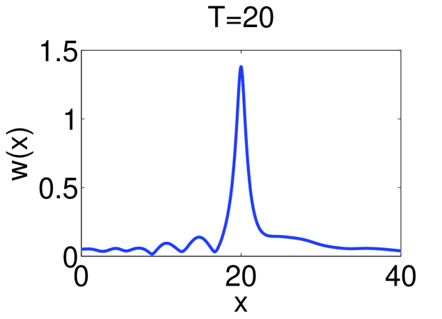
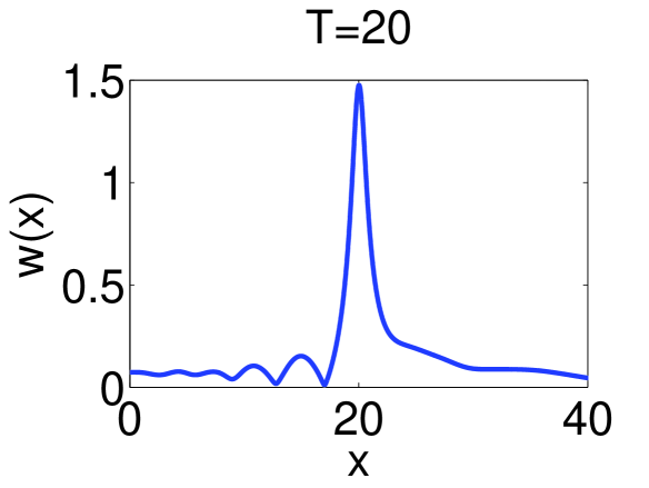
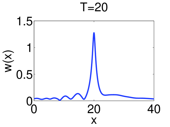
Figure 2: (Color online) (a,b,c): Density contour plots illustrating the dragging of the soliton, shown in Fig. 1(a), by the nonlinear trap with width $\epsilon=0.05$, moving as per Eq. (3), for three different values of the dragging time, $T$. The black solid lines show the corresponding trajectory $\xi(t)$. Adopting the criterion that the surviving soliton must keep $\geq 90\%$ of its initial amplitude, we conclude that it survives the transfer for $T\geq 20$. Panel (d) displays the shape of the soliton in the case of $T=20$, i.e., at the border of the survival, at time $t=30$ (some time after the completion of the transfer). Panels (e) and (f) display the same as (d), but for the moving trap with widths $\epsilon=0.1$ and $\epsilon=0.025$, respectively.

Results of the systematic simulations are summarized in Fig. 3, where the survival border is shown in the plane of the transfer parameters, $\Xi$ and $T$ [see Eq. (3)], for the fixed initial soliton and two different survival criteria, based on the demand of keeping the amplitude at the $90\%$ or $80\%$ level. It may again be concluded that the results are robust, as they only weakly depend on the particular choice of the criterion of the soliton’s survival. The roughly parabolic shape of the border may be explained by the fact that (as discussed in the previous section) the gradual destruction of the dragged soliton is determined by the absolute value of the acceleration of the moving trap. In the case of the motion law (3), the acceleration is

$$\frac{d^{2}\xi}{dt^{2}}=-\frac{\pi^{2}\Xi}{2T^{2}}\sin\left(\pi\frac{t-T/2}{T}\right),$$ (18)

hence its average absolute value in the process of the dragging is $\left\langle\left|d^{2}\xi/dt^{2}\right|\right\rangle=\pi\Xi/T^{2}$. Assuming that the soliton survives when the absolute value of the acceleration does not exceed a a certain critical level, the latter result predicts a parabolic shape of the survival border, $T\sim\sqrt{\Xi}$. To confirm the reasonable accuracy of the prediction, we have drawn a parabola with an empirically fitted coefficient, $T=\sqrt{7\pi\Xi}$ (the dashed line), to be compared to the numerically determined survival borders displayed in Fig. 3.

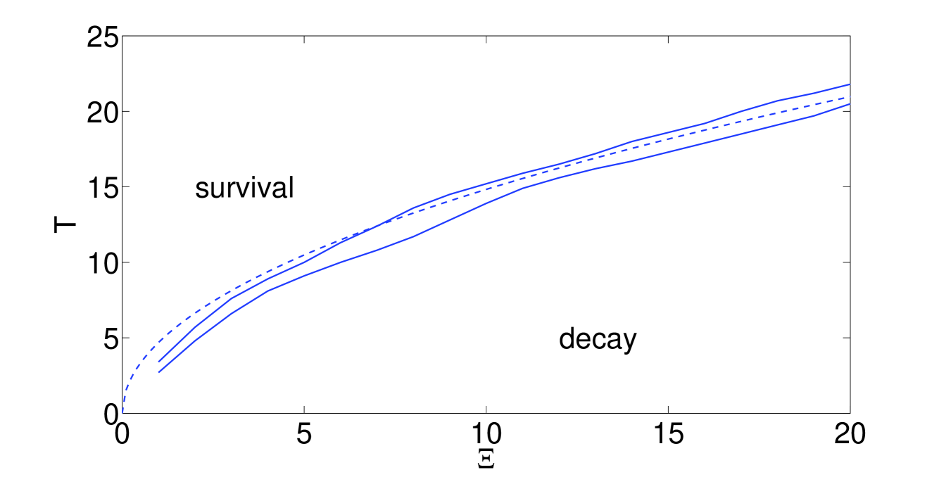
Figure 3: (Color online) The top and bottom solid curves represent the boundary above which the initial soliton with chemical potential $\mu=-1$, shown in Fig. 1(a), survives, keeping more than, respectively, $90\%$ or $80\%$ of the initial amplitude by $t=30$. The dashed curve depicts the analytical estimate (see text).

III.2 Quasi-Airy profiles dragged at a constant acceleration

We have also briefly studied profiles of waves dragged at a constant acceleration, i.e., those built as per Eqs. (12) and (15), and their stability within the framework of Eq. (10). A typical example of the stationary wave attached to the accelerating nonlinear $\delta$-function, i.e., a solution to Eq. (11), is displayed in Fig. 4. Direct simulations of Eq. (10) with this stationary wave used as the initial configuration were performed in order to examine its robustness. In particular, $a(z)$ was constructed and an approximate local minimum of the quantity $C_{1}^{2}+C_{2}^{2}$ [which determines the tail’s amplitude, $\left\langle a^{2}(z)\right\rangle$, as per Eq. (16)] was identified for appropriate values of $A$ and $z_{0}$. The temporal evolution of the resulting configuration is shown in Fig. 4.

A more detailed analysis of the quasi-Airy waves in the present nonlinear model will be a subject of a separate work. We note here that if we use small $A$ (such as $A=0.00057$ in the left column of Fig. 4), the apparent discontinuity of the beam at $z_{0}$ is barely visible; in this small-amplitude case, the solution appears to be more robust, and moves to the left, preserving its shape. If $A$ is larger ($A=1.14$ in the right panel), a significant fraction of the solution gets trapped by the delta-function at $z_{0}$, while the larger remaining fraction still moves to the left, and a smaller fraction of the initial power disperses to the right of $z_{0}$.

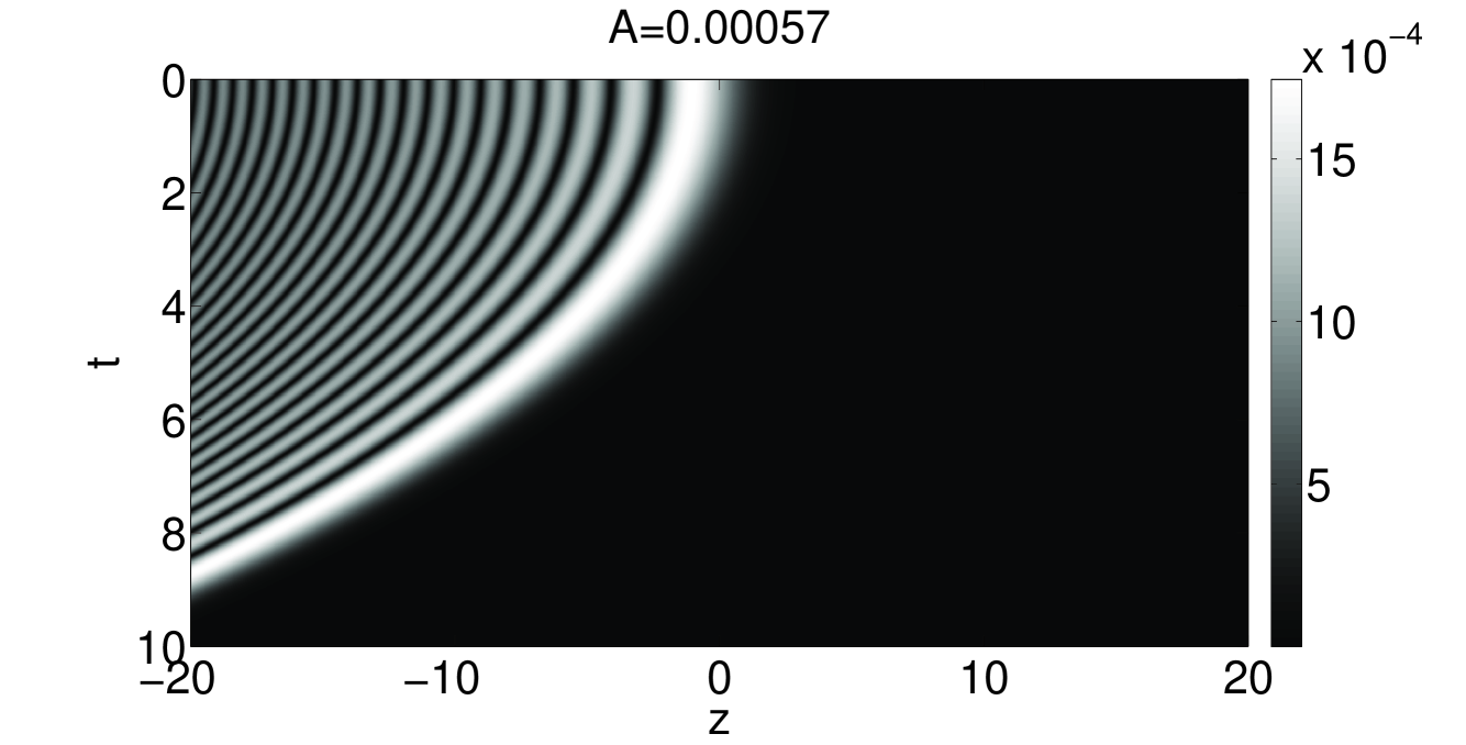
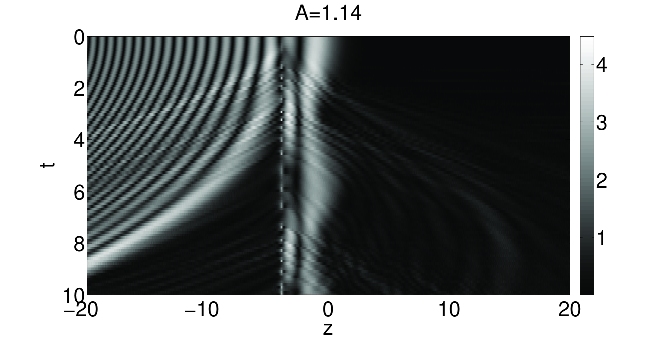
Figure 4: The temporal evolution of $a(z)$ with $z_{0}=-3.86235$, for the quasi-Airy waves dragged by the accelerating nonlinear trap with width $\epsilon=0.05$. The left and right panels show, respectively, the stationary solution with $A=0.00057$, and the unstable solution with $A=1.14$.

IV Scattering of coherent wave packets on the localized nonlinearity

The scattering problem in the framework of Eq. (1) with the ideal quiescent $\delta$-function was first studied in Ref. Azbel , where the scattering of an incident plane wave was considered. It was found that the localized self-attractive nonlinearity gave rise to an accordingly localized modulational instability (MI) of the incident wave, provided that its amplitude exceeded a certain threshold (minimum) value. Unlike the commonly known MI in the NLS equation with the uniform nonlinearity, the localized MI features a complex growth rate (i.e., it corresponds to the oscillatory instability).

Here, we aim to study the scattering from the regularized Gaussian nonlinear potential of incident wave packets in the form of coherent states. The latter represent the fundamental solutions of the linear Schrödinger equation in the free space,

$$\psi_{\mathrm{in}}(x,t)=\frac{B}{\sqrt{1+ibt}}\exp\left[-\frac{b\left(x-ct\right)^{2}}{1+ibt}+icx+\frac{ic^{2}}{2}t\right],$$ (19)

Here, $B$ and $b$ are real constants that determine, respectively, the amplitude and inverse width of the initial wave packet, $A=\left(1+b^{2}t^{2}\right)^{-1/4}B$ and $W=\sqrt{b^{-2}+t^{2}}$ are the same characteristics of the spreading packet; the norm of the packet is $N=\sqrt{\pi/(2b)}B^{2}$, while $c$ is its velocity. In particular, in the case of small $B^{2}$, the scattering problem may be considered in the Born’s approximation (see, e.g., Ref. saku ), by setting $\psi(x,t)=\psi_{\mathrm{in}}(x,t)+\psi_{\mathrm{Born}}\left(x,t\right)$, where the first correction is to be found from the linear inhomogeneous equation,

$$i\left(\psi_{\mathrm{Born}}\right)_{t}+\frac{1}{2}\left(\psi_{\mathrm{Born}}\right)_{xx}=-\delta(x)\left|\psi_{\mathrm{in}}\right|^{2}\psi_{\mathrm{in}}.$$ (20)

Equation (20) can be solved by means of the Fourier transform. Here, we instead focus on direct simulations of the scattering problem in a wide parametric region in the space of $(B,b)$, with the $\delta$-function regularized according to Eq. (2). As illustrated by the examples displayed in Fig. 5, the simulations demonstrate splitting of the incident wave packet into three parts—transmitted, trapped, and reflected ones. Naturally, the share of the trapped norm increases with $B$, i.e., with the enhancement of the nonlinearity; on the other hand, the dependence of the observed phenomenology on the inverse-width parameter $b$ is relatively weak. It is also worthy to mention that, as seen in Fig. 5(d), the trapped pulse performs oscillations around the localized nonlinearity, while the transmitted beam splits into jets—see Figs. 5(c,d).

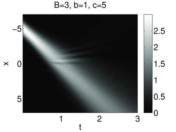
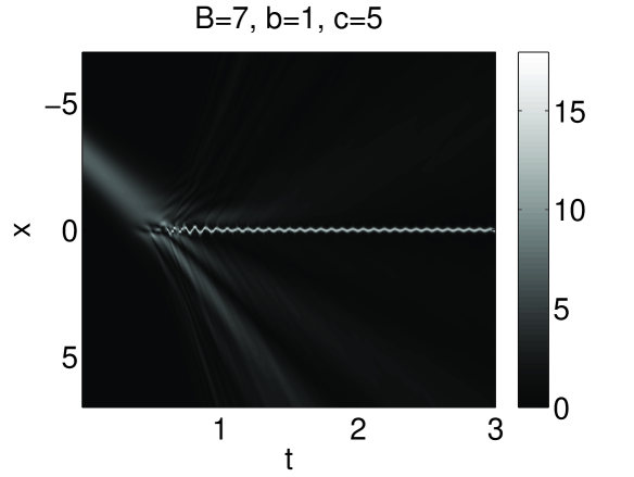
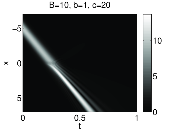
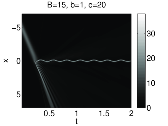
Figure 5: Examples of the interaction of the incident coherent pulse (19) with the localized nonlinear potential corresponding to the regularized profile (2), for $\epsilon=0.05$, at different values of the pulse’s amplitude and velocity.

Results of the simulations of the scattering are summarized in Figs. 6 and 7, where we show the shares of the trapped, reflected, and transmitted norm (or power, in terms of the optics model), as functions of the amplitude ($B$) and inverse width ($b$) of the incident pulse for a fixed velocity, $c=20$, and two different values of the scatterer’s width, $\epsilon=0.05$ and $0.1$, respectively. The plots correspond to the moment of time $t=0.5$, taken after the the incident pulse has passed the scatterer. Note that the sum of the three shares is, by construction, identically equal to $1$. Analysis of the numerical data demonstrates that, in the limit of large amplitude ($B$), the transmission decreases while the reflection of the wave packet from the nonlinear barrier gets enhanced.

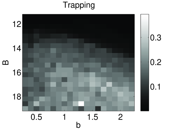
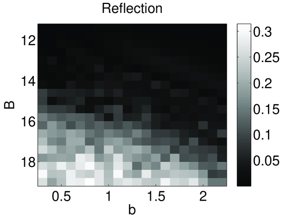
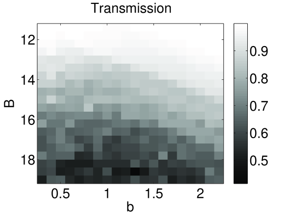
Figure 6: Panels (a), (b), and (c) display, by means of gray-scale plots, the trapped, reflected, and transmitted shares of the norm of the incident wave packet, as functions of its amplitude ($B$) and inverse width ($b$), for fixed velocity $c=20$ and width $\epsilon=0.05$ of the nonlinear scatterer, at the moment of time $t=0.5$. The trapped share is defined by the norm confined in interval $-1<x<+1$.

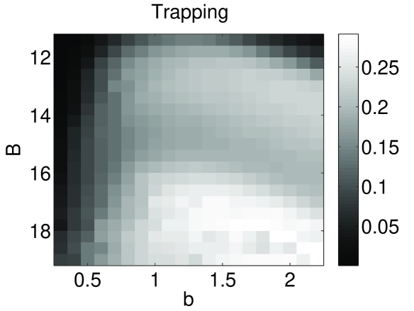
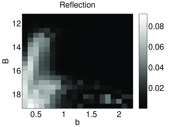
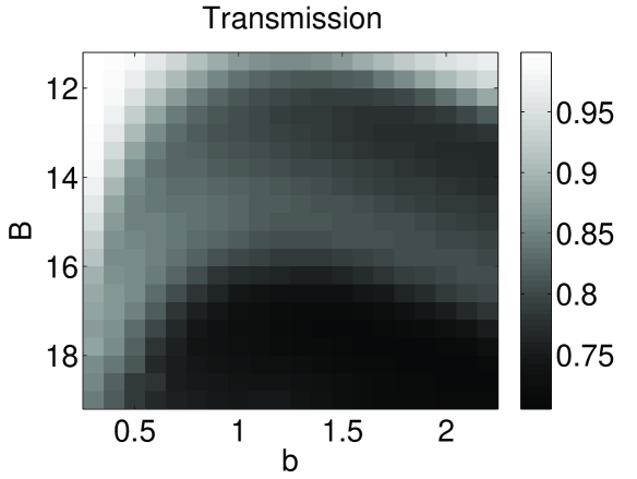
Figure 7: The same as in Fig. 6, but but for a broader scatterer, with $\epsilon=0.10$.

Further, the comparison of Figs. 6 and 7 shows that the increase of the width leads to a gradual change of the scattering picture. It is quite natural that the wider scatterer (Fig. 7) provides weaker reflection but stronger trapping of the incident waves. Generally, the solution of the scattering problem is more sensitive to the width $\epsilon$ than the results reported above for the transfer problem, as in the latter case the wave packet had a chance to adjust itself to the particular shape of the nonlinear scatterer.

V Conclusion

In this work, we have considered the 1D Schrödinger model with the tightly localized nonlinearity, to study the following dynamical problems: the existence and stability of standing waves trapped by this nonlinear potential; the controllable transfer of the localized mode by the moving nonlinear trap (nonlinear tweezers); and the scattering of coherent wave packets on the stationary localized nonlinearity. By means of systematic simulations, the border of the effective stability has been identified for the transfer problem. Relative shares of the norm (power) of the trapped, reflected, and transmitted waves were found, as functions of the amplitude and width of the incident pulse, for the scattering problem. The outcome of the transfer is less sensitive to particular characteristics of the nonlinear potential trap (such as its width) than the results of the solution of the scattering problem. The quasi-Airy stationary modes, dragged by the nonlinear trap moving at a constant acceleration, were briefly considered too, and were found to be progressively less robust for beams with the increasing amplitude. Some results were obtained in the approximate analytical form, such as the adiabatic approximation for the slowly dragged localized mode, and a qualitative explanation of the quasi-parabolic shape of the stability border.

This work may be naturally extended in other directions. It is especially interesting to consider the two-dimensional version of the transfer problem, using the corresponding localized nonlinear trap in the form of a circle Sakaguchi2 ; JMO and setting it in motion. A challenging issue in this case is the competition between the trapping of the two-dimensional wave packet, and its propensity to the intrinsic collapse. It may be also interesting to consider the scattering problem in one dimension in the case of a localized repulsive nonlinearity. Such studies will be reported in future publications.

References

- (1) T. Dauxois and M. Peyrard, Physics of Solitons (Cambridge University Press, Cambridge, 2006).
- (2) Y. V. Kartashov, B. A. Malomed, and L. Torner, Rev. Mod. Phys. 83, 247 (2011).
- (3) O. V. Borovkova, Y. V. Kartashov, B. A. Malomed, and L. Torner, Opt. Lett. 36, 3088 (2011); O. V. Borovkova, Y. V. Kartashov, L. Torner, and B. A. Malomed, Bright solitons from defocusing nonlinearities, Phys. Rev. E, in press.
- (4) W. A. Harrison, Pseudopotentials in the Theory of Metals (Benjamin: New York, 1966).
- (5) J. Hukriede, D. Runde, and D. Kip, J. Phys. D: Appl. Phys. 36, R1 (2003); K. Busch, G. von Freymann, S. Linden, S. F. Mingaleev, L. Tkeshelashvili, and M. Wegener, Phys. Rep. 444, 101 (2007).
- (6) C. R. Rosberg, F. H. Bennet, D. N. Neshev, P. D. Rasmussen, O. Bang, W. Królikowski, A. Bjarklev, and Y. S. Kivshar, Opt. Express 15, 12145 (2007).
- (7) S. Inouye, M. R. Andrews, J. Stenger, H. J. Miesner, D. M. Stamper-Kurn, and W. Ketterle, Nature 392, 151 (1998); Ph. Courteille, R. S. Freeland, D. J. Heinzen, F. A. van Abeelen, and B. J. Verhaar, Phys. Rev. Lett. 81, 69 (1998); J. L. Roberts, N. R. Claussen, J. P. Burke, C. H. Greene, E. A. Cornell, and C. E. Wieman, ibid. 81, 5109 (1998).
- (8) M. Marinescu and L. You, Phys. Rev. Lett. 81, 4596 (1998).
- (9) P. O. Fedichev, Yu. Kagan, G. V. Shlyapnikov, and J. T. M. Walraven, Phys. Rev. Lett. 77, 2913 (1996); M. Theis, G. Thalhammer, K. Winkler, M. Hellwig, G. Ruff, R. Grimm, and J. H. Denschlag, Phys. Rev. Lett. 93, 123001 (2004).
- (10) H. Sakaguchi and B. A. Malomed, Phys. Rev. E 72, 046610 (2005); J. Garnier and F. K. Abdullaev, Phys. Rev. A 74, 013604 (2006); D. L. Machacek, E. A. Foreman, Q. E. Hoq, P. G. Kevrekidis, A. Saxena, D. J. Frantzeskakis, and A. R. Bishop, Phys. Rev. E 74, 036602 (2006); M. A. Porter, P. G. Kevrekidis, B. A. Malomed, and D. J. Frantzeskakis, Physica D 229, 104 (2007); J. Belmonte-Beitia, V. M. Pérez-García, V. Vekslerchik, and P. J. Torres, Phys. Rev. Lett. 98, 064102 (2007); F. Abdullaev, A. Abdumalikov, and R. Galimzyanov, Phys. Lett. A 367, 149 (2007); G. Dong and B. Hu, Phys. Rev. A 75, 013625 (2007); D. A. Zezyulin, G. L. Alfimov, V. V. Konotop, and V. M. Pérez-García, ibid. 76, 013621 (2007); Z. Rapti, P. G. Kevrekidis, V. V. Konotop, and C. K. R. T. Jones, J. Phys. A: Math. Theor. 40, 14151 (2007); H. A. Cruz, V. A. Brazhnyi, and V. V. Konotop, J. Phys. B: At. Mol. Opt. Phys. 41, 035304 (2008); L. C. Qian, M. L. Wall, S. L. Zhang, Z. W. Zhou, and H. Pu, Phys. Rev. A 77, 013611 (2008); F. K. Abdullaev, A. Gammal, M. Salerno, and L. Tomio, ibid. 77, 023615 (2008); A. S. Rodrigues, P. G. Kevrekidis, M. A. Porter, D. J. Frantzeskakis, P. Schmelcher, and A. R. Bishop, ibid. 78, 013611 (2008); Y. V. Kartashov, B. A. Malomed, V. A. Vysloukh, and L. Torner, Opt. Lett. 34, 3625 (2009).
- (11) N. Dror and B. A. Malomed, Phys. Rev. A 83, 033828 (2011).
- (12) R. Y. Hao, R. C. Yang, L. Li, and G. S. Zhou, Opt. Commun. 281, 1256 (2008).
- (13) L. D. Carr and J. Brand, Phys. Rev. A 70, 033607 (2004); M. I. Rodas-Verde, H. Michinel, and V. M. Pérez-García, Phys. Rev. Lett. 95, 153903 (2005); P. Y. P. Chen and B. A. Malomed, J. Phys. B 38, 4221 (2005); ibid. 39, 2803 (2006); A. V. Carpentier, H. Michinel, M. I. Rodas-Verde, and V. M. Pérez-García, Phys. Rev. A 74, 013619 (2006); V. Pérez-García and R. Pardo, Physica D 238, 1352 (2009).
- (14) A. V. Carpentier, J. Belmonte-Beitia, H. Michinel, and M. I. Rodas-Verde, J. Mod. Opt. 55, 2819 (2008).
- (15) W. Guerin, J.-F. Riou, J. P. Gaebler, V. Josse, P. Bouyer, and A. Aspect, Phys. Rev. Lett. 97, 200402 (2006); N. P. Robins, C. Figl, M. Jeppesen, G. R. Dennis, and J. D. Close, Nature Phys. 4, 731 (2008).
- (16) H. Sakaguchi and B. A. Malomed, Phys. Rev. E 73, 026601 (2006).
- (17) G. Fibich, Y. Sivan, and M. I. Weinstein, Physica D 217, 31 (2006); G. Dong, B. Hu, and W. Lu, Phys. Rev. A 74, 063601 (2006); R. Y. Hao and G. S. Zhou, Chin. Opt. Lett. 6, 211 (2008); Y. V. Kartashov, B. A. Malomed, V. A. Vysloukh, and L. Torner, Opt. Lett. 34, 770 (2009); N. V. Hung, P. Ziń, M. Trippenbach, and B. A. Malomed, Phys. Rev. E 82, 046602 (2010).
- (18) T. Mayteevarunyoo, B. A. Malomed, and A. Reoksabutr, Spontaneous symmetry breaking of photonic and matter waves in two-dimensional pseudopotentials, J. Mod. Opt., in press.
- (19) B. A. Malomed and M. Ya. Azbel, Phys. Rev. B 47, 10402 (1993).
- (20) A. A. Sukhorukov, Y. S. Kivshar, and O. Bang, Phys. Rev. E 60, R41 (1999).
- (21) A. Shapira, N. Voloch-Bloch, B. A. Malomed, and A. Arie, J. Opt. Soc. Am. B 28, 1481 (2011).
- (22) T. Mayteevarunyoo, B. A. Malomed, and G. Dong, Phys. Rev. A 78, 053601 (2008).
- (23) V. A. Brazhnyi and B. A. Malomed, Phys. Rev. A 83, 053844 (2011); E. Bulgakov, K. Pichugin, and A. Sadreev, Phys. Rev. B 83, 045109 (2011).
- (24) M. I. Molina and G. P. Tsironis, Phys. Rev. B 47, 15330 (1993); B. C. Gupta and K. Kundu, ibid. 55, 894 (1997); 55, 11033 (1997).
- (25) R. Carretero-González, P. G. Kevrekidis, D. J. Frantzeskakis, and B. A. Malomed, in: Optical Trapping and Optical Micromanipulation II, edited by K. Dholakia and G. C. Spalding (SPIE, Bellingham, WA, 2005).
- (26) A. Marchewka and E. Granot, Phys. Rev. A 79, 012106 (2009); Europhys. Lett. 86, 20007 (2009); E. Sonkin, B. A. Malomed, E. Granot, and A. Marchewka, Phys. Rev. A 82, 033419 (2010).
- (27) A. del Campo, G. García-Calderón, and J. G. Muga, Phys. Rep. 476, 1 (2009).
- (28) H. A. Haus and W. S. Wong, Rev. Mod. Phys. 68, 423 (1996); S. Burtsev, D. J. Kaup, and B. A. Malomed, J. Opt. Soc. Am. B 13, 888 (1996).
- (29) M. V. Berry and N. L. Balazs, Am. J. Phys. 47, 264 (1979).
- (30) G. A. Siviloglou and D. N. Christodoulides, Opt. Lett. 32, 979 (2007); G. A. Siviloglou, J. Broky, A. Dogariu, and D. N. Christodoulides, Phys. Rev. Lett. 99, 213901 (2007).
- (31) T. Ellenbogen, N. Voloch-Bloch, A. Ganany-Padowicz, and A. Arie, Nature Photonics 3, 395 (2009); D. Abdollahpour, S. Suntsov, D. G. Papazoglou, and S. Tzortzakis, Phys. Rev. Lett. 105, 253901 (2010); Y. Hu, S. Huang, P. Zhang, C. Lou, J. Xu, and Z. Chen, Opt. Lett. 35, 3952 (2010).
- (32) E. Granot and B. A. Malomed, Acceleration of trapped particles and beams, J. Phys. B: At. Mol. Opt. Phys., in press.
- (33) R. Camassa and D. D. Holm, Phys. Rev. Lett. 71, 1661 (1993); A. Degasperis and M. Procesi, in: Symmetry and Perturbation Theory, A. Degasperis and G. Gaeta (eds.) (World Scientific, NJ, 1998).
- (34) L. Bergé, Phys. Rep. 303, 259 (1998).
- (35) M. Vakhitov and A. Kolokolov, Radiophys. Quantum. Electron. 16, 783 (1973).
- (36) Handbook of Mathematical Functions, ed. by M. Abramowitz and I. A. Stegun (National Bureau of Standards, 1964).
- (37) J. J. Sakurai, Modern quantum mechanics (Addison-Wesley, Reading MA, 1994).