Scalar Hair from a Derivative Coupling of a Scalar Field to the Einstein Tensor

Theodoros Kolyvaris ^†, George Koutsoumbas ^♯,
Eleftherios Papantonopoulos ^∗
Department of Physics, National Technical University of Athens,
Zografou Campus GR 157 73, Athens, Greece
George Siopsis ^♭

Department of Physics and Astronomy, The University of Tennessee,
Knoxville, TN 37996 - 1200, USA

We consider a gravitating system of vanishing cosmological constant consisting of an electromagnetic field and a scalar field coupled to the Einstein tensor. A Reissner-Nordström black hole undergoes a second-order phase transition to a hairy black hole of generally anisotropic hair at a certain critical temperature which we compute. The no-hair theorem is evaded due to the coupling between the scalar field and the Einstein tensor. Within a first order perturbative approach we calculate explicitly the properties of a hairy black hole configuration near the critical temperature and show that it is energetically favorable over the corresponding Reissner-Nordström black hole.

${}^{\dagger}~{}~{}$ e-mail address: teokolyv@central.ntua.gr

${}^{\sharp}~{}~{}$ e-mail address: kutsubas@central.ntua.gr

${}^{*}~{}~{}$ e-mail address: lpapa@central.ntua.gr

${}^{\flat}~{}~{}$ e-mail address: siopsis@tennessee.edu

1 Introduction

The “no-hair” theorems are powerful tools in studying black hole solutions of Einstein gravity coupled with matter. These “no-hair” theorems describe the existence and stability of four-dimensional asymptotically flat black holes coupled to an electromagnetic field or in vacuum. In the case of a minimally coupled scalar field in asymptotically flat spacetime the “no-hair” theorems were proven imposing conditions on the form of the self-interaction potential [1]. These theorems were also generalized to non-minimally coupled scalar fields [2].

For asymptotically flat spacetime, a four-dimensional black hole coupled to a scalar field with a zero self-interaction potential is known [3]. However, the scalar field diverges on the event horizon and, furthermore, the solution is unstable [4], so there is no violation of the “no-hair” theorems. In the case of a positive cosmological constant with a minimally coupled scalar field with a self-interaction potential, black hole solutions were found in [5] and also a numerical solution was presented in [6], but it was unstable. If the scalar field is non-minimally coupled, a solution exists with a quartic self-interaction potential [7], but it was shown to be unstable [8, 9].

In the case of a negative cosmological constant, stable solutions were found numerically for spherical geometries [10, 11] and an exact solution in asymptotically AdS space with hyperbolic geometry was presented in [12] and generalized later to include charge [13] and further generalized to non-conformal solutions [14]. This solution is perturbatively stable for negative mass and may develop instabilities for positive mass [15]. The thermodynamics of this solution was studied in [12] where it was shown that there is a second order phase transition of the hairy black hole to a pure topological black hole without hair. The analytical and numerical calculation of the quasi-normal modes of scalar, electromagnetic and tensor perturbations of these black holes confirmed this behaviour [16]. Recently, a new exact solution of a charged C-metric conformally coupled to a scalar field was presented in [17, 18]. A Schwarzschild-AdS black hole in five-dimensions coupled to a scalar field was discussed in [19], while dilatonic black hole solutions with a Gauss-Bonnet term in various dimensions were discussed in [20].

Recently scalar-tensor theories with nonminimal couplings between derivatives of a scalar field and curvature were studied. The most general gravity Lagrangian linear in the curvature scalar R, quadratic in the scalar field $\phi$, and containing terms with four derivatives was considered in [21]. It was shown that this theory cannot be recast into Einsteinian form by a conformal rescaling. It was further shown that without considering any effective potential, an effective cosmological constant and then an inflationary phase can be generated.

Subsequently it was found [22] that the equation of motion for the scalar field can be reduced to a second-order differential equation when the scalar field is kinetically coupled to the Einstein tensor. Then the cosmological evolution of the scalar field coupled to the Einstein tensor was considered and it was shown that the universe at early stages has a quasi-de Sitter behaviour corresponding to a cosmological constant proportional to the inverse of the coupling of the scalar field to the Einstein tensor. These properties of the derivative coupling of the scalar field to curvature had triggered the interest of the study of the cosmological implications of this new type of scalar-tensor theory [23, 24, 25, 26]. Also local black hole solutions were discussed in [27].

The dynamical evolution of a scalar field coupled to the Einstein tensor in the background of a Reissner-Nordström black hole was studied in [28]. By calculating the quasinormal spectrum of scalar perturbations it was found that for weak coupling of the scalar field to the Einstein tensor and for small angular momentum the effective potential outside the horizon of the black hole is always positive indicating that the background black hole is stable for a weaker coupling. However, for higher angular momentum and as the coupling constant gets larger than a critical value, the effective potential develops a negative gap near the black hole horizon indicating an instability of the black hole background.

The previous discussion indicates that the presence of the derivative coupling of a scalar field to the Einstein tensor on cosmological or black hole backgrounds generates an effect similar to the presence of an effective cosmological constant. In this paper we investigate this effect further. We consider a spherically symmetric Reissner-Nordström black hole and perturb this background by introducing a derivative coupling of a scalar field to the Einstein tensor. We show that in this gravitating system there exists a critical temperature in which the system undergoes a second-order phase transition to an anisotropic hairy black hole configuration and the scalar field is regular on the horizon. This “Einstein hair” is the result of evading the no-hair theorem thanks to the presence of the derivative coupling of the scalar field to the Einstein tensor.

The coupled dynamical system of Einstein-Maxwell-Klein-Gordon equations is a highly non-linear system of equations for which even a numerical solution appears beyond reach. To solve the field equations, we expand the fields around a Reissner-Nordström black hole solution and pertubatively determine the critical temperature. By solving the first-order equations numerically near the critical temperature, we study the behaviour of the hairy black hole solution. We calculate the temperature of the new hairy black hole and compare it with the corresponding temperature of a Reissner-Nordström black hole of the same charge. We find that above the critical temperature the Reissner-Nordström black hole is unstable and by calculating the free energies we show that the new hairy black hole configuration is energetically favorable over the corresponding Reissner-Nordström black hole.

The paper is organized as follows. In Sec. 2 we set up the field equations and outline our solution. In Sec. 3 we find the zeroth order solution and calculate the critical temperature near which the Reissner-Nordström black hole may become unstable and develop hair. In Sec. 4 we find the first-order solutions to the system of Einstein-Maxwell-Klein-Gordon equations which are hairy black holes near the critical temperature. In Sec. 5 we discuss the thermodynamic stability of our first-order hairy solution. In Sec. 6 we discuss the validitiy of our perturbative expansion. Finally, in Sec. 7 we conclude.

2 The field equations

Consider the Lagrangian density

$$\mathcal{L}=\frac{R}{16\pi G}-\frac{1}{4}F_{\mu\nu}F^{\mu\nu}-(g^{\mu\nu}+\kappa G^{\mu\nu})D_{\mu}\varphi(D_{\nu}\varphi)^{*}-m^{2}|\varphi|^{2}~{},$$ (2.1)

where $D_{\mu}=\partial_{\mu}-ieA_{\mu}$ and $e$, $m$ the charge and mass of the scalar field and $\kappa$ the coupling of the scalar field to Einstein tensor, of dimension length squared.

In this paper, we shall concentrate on the case of a massless and chargeless scalar field, setting

$$m=0\ \ ,\ \ \ \ e=0~{},$$ (2.2)

and leave the study of the general case to future work. Consequently, the scalar field $\varphi$ is real.

With the choice of parameters (2.2), the field equations resulting from the Lagrangian (2.1) are the Einstein equations

$$R_{\mu\nu}=8\pi GT_{\mu\nu}~{},$$ (2.3)

the Maxwell equations

$$\nabla^{\mu}F_{\mu\nu}=0\ ,\ \ F_{\mu\nu}=\partial_{\mu}A_{\nu}-\partial_{\nu}A_{\mu}~{},$$ (2.4)

and the Klein-Gordon equation for the scalar field,

$$\frac{1}{\sqrt{-g}}\partial_{\mu}\left[\sqrt{-g}(g^{\mu\nu}+\kappa G^{\mu\nu})\partial_{\nu}\varphi\right]=0~{}.$$ (2.5)

The stress-energy tensor receives three contributions,

$$T_{\mu\nu}=T_{\mu\nu}^{(EM)}+T_{\mu\nu}^{(\varphi)}+\kappa\Theta_{\mu\nu}~{},$$ (2.6)

where $T_{\mu\nu}^{(EM)}$ is the electromagnetic stress-energy tensor, $T_{\mu\nu}^{(\varphi)}$ is the standard scalar field contribution,

$$T_{\mu\nu}^{(\varphi)}=\partial_{\mu}\varphi\partial_{\nu}\varphi-\frac{1}{2}g_{\mu\nu}g^{\alpha\beta}\partial_{\alpha}\varphi\partial_{\beta}\varphi~{},$$ (2.7)

and $\Theta_{\mu\nu}$ is an extra matter source resulting from the derivative coupling of the scalar field to the Einstein tensor,

$$\Theta_{\mu\nu} = -\frac{1}{2}\nabla_{\mu}\varphi\nabla_{\nu}\varphi R-\frac{1}{2}(\nabla\varphi)^{2}G_{\mu\nu}+\frac{1}{2}\nabla_{\mu}\nabla_{\nu}(\nabla\varphi)^{2}-\frac{1}{2}g_{\mu\nu}\square(\nabla\varphi)^{2}$$ (2.8)

$$-\frac{1}{2}g_{\mu\nu}\nabla_{\alpha}\varphi\nabla_{\beta}\varphi R^{\alpha\beta}+2\nabla_{\alpha}\varphi\nabla_{(\mu}\varphi R_{\nu)}^{\alpha}+\frac{1}{2}\square(\nabla_{\mu}\varphi\nabla_{\nu}\varphi)-\nabla_{\alpha}\nabla_{(\mu}(\nabla_{\nu)}\varphi\nabla^{\alpha}\varphi)$$

$$+\frac{1}{2}g_{\mu\nu}\nabla_{\alpha}\nabla_{\beta}(\nabla^{\alpha}\varphi\nabla^{\beta}\varphi)~{}.$$

The field equations have well-known solutions for $\varphi=0$, the Reissner-Nordström black holes. We are interested in finding hairy solutions, with $\varphi\neq 0$. The no-hair theorem will be evaded thanks to the coupling of the scalar field to the Einstein tensor (“Einstein hair”).

To solve the non-linear field equations, we shall expand around a Reissner-Nordström black hole. It should be pointed out that not all Reissner-Nordström black holes can be starting points of such a perturbative expansion. We will show that for a given charge of the black hole, there is generally a unique mass for which the Reissner-Nordström black hole can be a starting point. The corresponding temperature is then expected to be a critical temperature at which a phase transition occurs from a Reissner-Nordström black hole to a hairy one.

Introducing the (small) order parameter $\varepsilon$, we therefore set

$$\varphi = \varepsilon\left(\varphi^{(0)}+\varepsilon^{2}\varphi^{(1)}+\dots\right)$$

$$g_{\mu\nu} = g_{\mu\nu}^{(0)}+\varepsilon^{2}g_{\mu\nu}^{(1)}+\dots$$

$$A_{\mu} = A_{\mu}^{(0)}+\varepsilon^{2}A_{\mu}^{(1)}+\dots$$ (2.9)

and solve the field equations perturbatively.

To find a static solution of the field equations, it is convenient to consider the metric ansatz

$$ds^{2}=-e^{-\alpha}dt^{2}+l^{2}e^{\alpha}\left[e^{-\beta}(dr^{2}+r^{2}d\theta^{2})+r^{2}\sin^{2}\theta d\phi^{2}\right]~{},$$ (2.10)

and electromagnetic potential

$$A_{t}=A(r,\theta)\ \ ,\ \ \ \ \vec{A}=\vec{0}~{}.$$ (2.11)

The metric functions are expanded as

$$l = l_{0}+\varepsilon^{2}l_{1}+\dots$$

$$\alpha = \alpha_{0}+\varepsilon^{2}\alpha_{1}+\dots$$

$$\beta = \beta_{0}+\varepsilon^{2}\beta_{1}+\dots~{},$$ (2.12)

and the electrostatic potential as

$$A=A_{0}+\varepsilon^{2}A_{1}+\dots~{}.$$ (2.13)

The components of the electromagnetic stress-energy tensor are

$$T_{t}^{(EM)t}=-T_{\phi}^{(EM)\phi} = \frac{1}{2r^{2}l^{2}g}\left[r^{2}(\partial_{r}A)^{2}+(\partial_{\theta}A)^{2}\right]~{},$$

$$T_{r}^{(EM)r}=-T_{\theta}^{(EM)\theta} = \frac{1}{2r^{2}l^{2}g}\left[r^{2}(\partial_{r}A)^{2}-(\partial_{\theta}A)^{2}\right]~{},$$

$$T_{r}^{(EM)\theta} = \frac{1}{l^{2}g}\partial_{r}A\partial_{\theta}A~{}.$$ (2.14)

The Einstein equations reduce to the convenient subset

$$R_{t}^{t}+R_{\phi}^{\phi} = 8\pi G\left(T_{t}^{t}+T_{\phi}^{\phi}-T\right)~{},$$ (2.15)

$$R_{t}^{t} = 8\pi G\left(T_{t}^{t}-\frac{1}{2}T\right)~{},$$ (2.16)

$$R_{r}^{r}-R_{\theta}^{\theta} = 8\pi G\left(T_{r}^{r}-T_{\theta}^{\theta}\right)~{},$$ (2.17)

where

$$T=T_{\mu}^{\mu}=-(\partial\varphi)^{2}~{},$$ (2.18)

to be solved together with the Maxwell equation (Gauss’s Law),

$$\nabla_{\mu}\nabla^{\mu}A=0~{}.$$ (2.19)

and the Klein-Gordon equation (2.5).

The Hawking temperature of the black hole solution can also be expanded as

$$T=T_{0}+\varepsilon^{2}T_{1}+\dots~{}.$$ (2.20)

When $\varepsilon=0$, the temperature is $T=T_{0}$. This is a critical temperature at which a second-order phase transition occurs to a hairy black hole, if the latter solution exists and is energetically favorable. For a small order parameter,

$$\varepsilon\sim|T-T_{0}|^{1/2}~{},$$ (2.21)

so our expansion can be viewed as an expansion around the critical temperature.

Next, we proceed with the perturbative solution of the field equations.

3 Zeroth order solution

At zeroth order we obtain the Einstein-Maxwell equations

$$R_{\mu\nu}^{(0)}=8\pi GT_{\mu\nu}^{(EM)(0)}\ ,\ \ \nabla^{\mu}F_{\mu\nu}^{(0)}=0~{},$$ (3.1)

as well as the Klein-Gordon equation

$$\frac{1}{\sqrt{-g^{(0)}}}\partial_{\mu}\left[\sqrt{-g^{(0)}}(g^{(0)\mu\nu}+\kappa R^{(0)\mu\nu})\partial_{\nu}\varphi^{(0)}\right]=0~{},$$ (3.2)

where we used $G_{\mu\nu}^{(0)}=R_{\mu\nu}^{(0)}$ for the solution of (3.1). Thus at this order, the Einstein-Maxwell equations decouple (effectively, $\varepsilon=0$), and the solution $g_{\mu\nu}^{(0)}$, $A_{\mu}^{(0)}$ has no hair (e.g., a Reissner-Nordström black hole).

Note the Klein-Gordon equation for $\varphi^{(0)}$ in the background $(g_{\mu\nu}^{(0)}\ ,\ A_{\mu}^{(0)})$ constrains the background, because not all solutions of the Einstein-Maxwell equations lead to regular functions $\varphi^{(0)}$. The demand of regularity results in relations among the parameters of the Reissner-Nordström solution. Viewed as a thermodynamic system, the critical temperature $T_{0}$ is also constrained by demanding regularity of $\varphi^{(0)}$.

The Einstein-Maxwell equations at zeroth order (3.1) have as a solution the Reissner-Nordström black hole. In Lewis-Papapetrou coordinates,

$$l_{0}=1-\frac{\mu^{2}}{r^{2}}\ ,\ \ l_{0}e^{\alpha_{0}/2}=1+\frac{\mu^{2}}{r^{2}}+\frac{2\mu\coth B}{r}\ ,\ \ \beta_{0}=0~{},$$ (3.3)

and the electrostatic potential is

$$A_{t}^{(0)}=\Phi-\frac{Q}{rl_{0}}e^{-\alpha_{0}/2}\ \ ,\ \ \ \ Q=\frac{2\mu}{\sqrt{G}\,\sinh B}\ ,\ \ \Phi=\frac{e^{-B}}{\sqrt{G}}~{},$$ (3.4)

where $Q$ is the charge of the black hole, and $\Phi$ is the value of the potential as $r\to\infty$, fixed by the requirement that $A_{\mu}A^{\mu}$ be finite at the horizon.

To put it in more familiar terms, performing the coordinate transformation

$$\rho=l_{0}re^{\alpha_{0}/2}=r+\frac{\mu^{2}}{r}+2\mu\coth B~{},$$

the metric becomes

$$ds^{2}=-f(\rho)dt^{2}+\frac{d\rho^{2}}{f(\rho)}+\rho^{2}d\Omega^{2}\ \ ,\ \ \ \ f(\rho)=1-\left(1+\frac{GQ^{2}}{\rho_{+}^{2}}\right)\frac{\rho_{+}}{\rho}+\frac{GQ^{2}}{\rho^{2}}~{},$$ (3.5)

showing that the horizon is at $\rho=\rho_{+}$ ,

$$\rho_{+}=Q\sqrt{G}\ e^{B}~{}.$$

The electrostatic potential reads $A_{t}^{(0)}=\frac{Q}{\rho}$, confirming that $Q$ is the charge of the hole. Its temperature is

$$T=\frac{f^{\prime}(\rho_{+})}{4\pi}=\frac{1}{4\pi\rho_{+}}\left(1-\frac{GQ^{2}}{\rho_{+}^{2}}\right)=\frac{e^{-2B}\sinh^{2}B}{4\pi\mu}~{}.$$ (3.6)

The mass, entropy, and potential are, respectively,

$$M=\frac{2\mu}{G}\coth B\ \ ,\ \ \ \ S=\frac{4\pi\mu^{2}}{G}\frac{e^{2B}}{\sinh^{2}B}\ \ ,\ \ \ \ \Phi=\frac{e^{-B}}{\sqrt{G}}~{}.$$ (3.7)

From these, or using the Euclidean action, we deduce the Gibbs free energy

$$F=M-TS-Q\Phi=\frac{\mu}{G}~{}.$$ (3.8)

Additionally, the scalar field obeys the Klein-Gordon equation (3.2). For $\kappa=0$, there is no regular solution, which is a consequence of the no-hair theorem [1, 2]. However, for $\kappa\neq 0$, we obtain regular static solutions for certain values of the parameters $\mu$ and $B$. In [28] the Klein-Gordon equation (3.2) was solved numerically in the background of the Reissner-Nordström black hole. The corresponding temperature of the Reissner-Nordström black hole $T_{0}$ is the critical temperature, near which the black hole may become unstable and develop hair, evading the no-hair theorem.

To calculate the critical temperature, it is convenient to introduce the coordinate

$$z=\frac{\mu}{r}~{},$$ (3.9)

so that the boundary is at $z=0$ and the horizon at $z=1$.

We look for regular solutions of the Klein-Gordon equation (3.2) in the interval $[0,1]$. Such solutions where discussed in [28] where an instability was found in the quasinormal frequencies for multipole number $\ell\neq 0$. To capture such an effect we consider a non-spherical ansatz

$$\varphi^{(0)}=\mathcal{Z}(z)P_{\ell}(\cos\theta)~{}.$$ (3.10)

After some straightforward algebra, we obtain

$$\frac{z^{2}}{l_{0}}\left(l_{0}(1+\kappa\mathcal{R})\mathcal{Z}^{\prime}\right)^{\prime}-(1-\kappa\mathcal{R})\ell(\ell+1)\mathcal{Z}=0~{},$$ (3.11)

where prime denotes differentiation with respect to $z$ and we defined

$$\mathcal{R}={R^{(0)}}_{t}^{t}={R^{(0)}}_{z}^{z}=-{R^{(0)}}_{\theta}^{\theta}=\frac{8\sinh^{2}B}{\mu^{2}}\frac{z^{4}}{[(1+z^{2})\sinh B+2z\cosh B]^{4}}~{}.$$ (3.12)

The Klein-Gordon equation (3.2) does not have a solution with a regular scalar field at the horizon for $\ell=0$. This means that scalar hair, if it exists, is anisotropic. We shall concentrate on the case of a dipole,

$$\ell=1~{}.$$ (3.13)

At the boundary we obtain $z^{2}\mathcal{Z}^{\prime\prime}-\ell(\ell+1)\mathcal{Z}\approx 0$, therefore

$$\mathcal{Z}\sim z^{\ell+1}~{}.$$

At the horizon we have $((1-z)\mathcal{Z}^{\prime})^{\prime}\approx 0$, therefore $\mathcal{Z}^{\prime}\sim 0$ or $\mathcal{Z}^{\prime}\sim\frac{1}{1-z}$. For each value of the charge $Q$, there should be a unique combination of parameters $\mu$ and $B$ that gives a convergent $\mathcal{Z}^{\prime}$ (and therefore a finite $\mathcal{Z}$) at the horizon. For given $\kappa$, we will determine numerically pairs of $\mu$ and $B$ from (3.11) and their values will be used to determine $T_{0}$ as a function of the charge $Q$ using (3.6).

To solve the scalar wave equation (3.11) numerically, we use the variational method. In particular we use an expansion around the horizon

$$\mathcal{Z}(z)=z^{2}W(z)=z^{2}\sum_{n=0}^{\infty}W_{n}(1-z)^{n}~{}.$$ (3.14)

It turns out that for a better than 10% precision, one needs to keep at least 10 terms in the expansion.

The coefficients $W_{n}$ depend on $\kappa$ and $B.$ Our aim is to find a unique $\kappa$ which will give finite $\mathcal{Z}(z)$ and $\mathcal{Z}(z)^{\prime}$ at the horizon $z=1.$ One may rearrange eq. (3.11) to get

$$\kappa=\frac{\int_{0}^{1}dz(1-z^{2})[2\mathcal{Z}(z)^{2}/z^{2}+\mathcal{Z}^{\prime 2}(z)]}{\int_{0}^{1}dz(1-z^{2}){\cal R}(z)[2\mathcal{Z}(z)^{2}/z^{2}-\mathcal{Z}^{\prime 2}(z)]}~{},$$ (3.15)

which can be solved graphically. For the choice

$$\kappa=10\ ,\ \ Q=9.5~{},$$ (3.16)

in units in which $8\pi G=1$, we obtain $\mu=0.15$, $B=0.158$ (see figure 1), which gives the critical temperature

$$T_{0}\approx 0.01~{}.$$ (3.17)

In figure 2, we depict the scalar function $\mathcal{Z}(z)$ for the chosen values of the parameters, normalized so that $\mathcal{Z}(1)\sim T_{0}$ (the scalar field and the temperature have the same dimension). The normalization is arbitrary, since the wave equation is linear.

The function $\mathcal{Z}(z)$ is regular in the entire range outside the horizon, as desired.

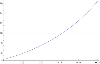
Figure 1: Graphical solution of (3.15) vs. $B$, showing that $B=0.158$.

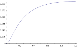
Figure 2: The function ${\cal Z}(z)$ for the scalar field versus $z$ for the parameters of figure 1.

Figure 3: The critical temperature $T_{0}$ vs. the charge $Q$ for various values of $\kappa.$ Black squares correspond to $\kappa=15,$ white squares to $\kappa=10,$ while there follow $\kappa=5,\ \kappa=3$ and $\kappa=1.$

For the first order numerical solutions of the next section we used the values of $\kappa$ and $Q$ given in (3.16). However, to show how the critical temperature depends on the parameters, in figure 3 we show the results of a numerical study of the critical temperature $T_{0}$ as a function of the black hole charge $Q$ for various values of the Einstein coupling constant $\kappa$, ranging from $\kappa=1$ to $\kappa=15$. The critical temperature diverges as $Q\to 0$ (Schwarzschild limit) for all values of $\kappa$.

4 First order solution

At first order, the field equations yield a solution near the critical temperature, where the scalar field $\varphi$ backreacts on the metric.

To extract the first-order equations from the full set of non-linear field equations, notice that the stress-energy tensor to this order has contributions from the electromagnetic stress-energy tensor (2.14), and the scalar field (eqs. (2.7) and (2.8), with $\varphi$ replaced by $\varepsilon\varphi^{(0)}$ and $g_{\mu\nu}$ replaced by the RN solution $g_{\mu\nu}^{(0)}$). For the contribution (2.8), after some algebra we obtain the explicit expression

$$\Theta_{t}^{t}=\Theta_{z}^{z}=-\Theta_{\theta}^{\theta}=-\Theta_{\phi}^{\phi}=\varepsilon^{2}\frac{2z^{6}e^{-3\alpha}}{\mu^{4}l_{0}^{6}\sinh^{2}B}\left[z^{2}{\mathcal{Z}^{\prime}}^{2}\cos^{2}\theta+\mathcal{Z}^{2}\sin^{2}\theta\right]+\mathcal{O}(\varepsilon^{4})~{}.$$ (4.1)

We give the technical details of the solution of the equations (2.15)-(2.19) in Appendix A. Having the solutions of the equations (2.15)-(2.19) we will numerically determine the metric functions $\alpha$ and $\beta$ and the electric potential $A$. Notice that the order parameter $\varepsilon$ and the normalization of the zeroth-order scalar field $\varphi^{(0)}$ are not independently defined, since only their product (which ought to be small for the perturbative expansion to be valid) enters the field equations. For convenience, we set $\varepsilon=1$ in our numerical calculations, making the normalization of $\varphi^{(0)}$ small.

We wand to find the functions $\alpha_{10}(z)$, $A_{10}(z)$, $\alpha_{12}(z)$, $A_{12}(z)$ which appear in the first order corrections

$$\alpha_{1} = \alpha_{10}(z)P_{0}(\cos\theta)+\alpha_{12}(z)P_{2}(\cos\theta)~{},$$

$$A_{1} = A_{10}(z)P_{0}(\cos\theta)+A_{12}(z)P_{2}(\cos\theta)~{}.$$ (4.2)

We will calculate first the angle-independent first-order corrections. For the correction $\alpha_{10}$ we work with equation (A.12) noticing that at the boundary $\alpha_{10}(z)\sim\lambda z,$ while at the horizon such a solution yields an expression $a+b\ln(1-z).$ Fine tuning of $\lambda$ will yield $b=0,$ that is, a regular solution. On the technical side we change the variable $\alpha_{10}$ to $\zeta_{0}\equiv\frac{\alpha_{10}}{z}$ with the new boundary conditions $\zeta_{0}(0)=\lambda,\ \zeta_{0}^{\prime}(0)=0.$ Figure 4 depicts the results for $\alpha_{10}$ for $\lambda=-0.000421852,$ which is found to yield a regular solution.

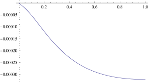
Figure 4: The function $\alpha_{10}(z)$ of the angle-independent part of the first-order correction to the metric.

The first-order correction to the electric potential $A(z)=A_{0}+\varepsilon^{2}A_{10}$ may be directly determined if $\alpha$ is known using (A.11) and the result is plotted in figure 5.

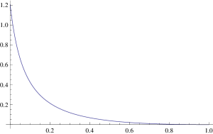
Figure 5: The electrostatic potential $A(z)$ at first order.

A procedure similar to the one used for the scalar field will be used for the solution of the equations (LABEL:A2) and (LABEL:a2) for the angle-dependent first order corrections $A_{12}$ and $\alpha_{12}.$ We use the expansions:

$$\alpha_{12}(z)=z^{3}\sum_{n=1}^{\infty}\tilde{\alpha}_{12}^{(n)}(1-z)^{n},\ \ \ A_{12}(z)=z^{3}\sum_{n=1}^{\infty}\tilde{A}_{12}^{(n)}(1-z)^{n},$$ (4.3)

where $\tilde{\alpha}_{12}^{(n)},\ \tilde{A}_{12}^{(n)}$ depend on a single free parameter which can be chosen to be $\tilde{A}_{12}^{(2)}$ (it is easily seen that the first term vanishes, $\tilde{A}_{12}^{(1)}=0$). This parameter can be determined by a variational method. To this end, multiply (LABEL:A2) by $A_{12}$ and integrate. We obtain

$$\int_{0}^{1}dz\left[-(A_{12}^{\prime})^{2}-\left(-\frac{l^{2}}{z^{2}D^{2}}+\frac{2}{z^{2}D}-\frac{1-3z^{2}}{z^{2}l_{0}^{2}}+\frac{6}{z^{2}}\right)A_{12}^{2}+\frac{Ql_{0}}{\mu D^{2}}A_{12}\alpha_{12}^{\prime}\right]=0$$ (4.4)

where we defined

$$D(z)=1+z^{2}+2z\coth B~{}.$$ (4.5)

Similarly, if we multiply (LABEL:a2) by $\alpha_{12}$, we obtain

$$\int_{0}^{1}dz\left[-(\alpha_{12}^{\prime})^{2}-\left(-\frac{1+z^{2}}{l_{0}^{2}}+\frac{6}{z^{2}}+\frac{8}{(D\sinh B)^{2}}\right)\alpha_{12}^{2}+\frac{16\pi GQ}{\mu l_{0}}\alpha_{12}A_{12}^{\prime}-16\pi G\frac{\kappa\mathcal{Q}_{2}}{z^{2}}\alpha_{2}\right]=0~{}.$$ (4.6)

Both of these equations must be satisfied at the right value of $\tilde{A}_{12}^{(2)}$. Either one of them determines this value.

In figure 6 we show the results for the variational expressions versus the undetermined parameter $\tilde{A}_{12}^{(2)}$ and find that $\tilde{A}_{12}^{(2)}=0.2.$ We depict the left-hand side of (4.6) and the sum of (4.4) and (4.6) keeping four terms in each of the expansions (4.3). Notice that the two curves are almost indistinguishable and both approach zero at the same value, confirming the consistency of our numerical approach. In figure 7 we depict the solution for $A_{12},$ while in figure 8 the solution for $\alpha_{12}.$ Therefore, the first order corrections $A_{12}$ and $\alpha_{12}$ are regular everywhere.

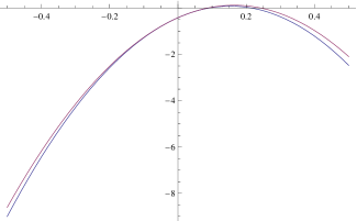
Figure 6: Variational expressions (4.4) and (4.6) vs. $\tilde{A}_{12}^{(2)}$ showing that $\tilde{A}_{12}^{(2)}=0.2.$

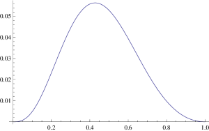
Figure 7: The function $A_{12}(z)$ for the parameters of figure 1 and $\tilde{A}_{12}^{(2)}=0.2.$

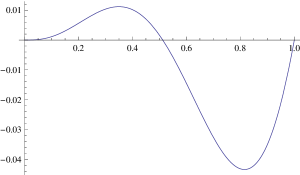
Figure 8: The function $\alpha_{12}(z)$ for the parameters of figure 1 and $\tilde{A}_{12}^{(2)}=0.2.$

Finally, the metric function $\beta$ which is given by (A.18) has as the first order angle-independent correction the function $\beta_{10}$ of (A.23) which is shown in figure 9. The function $\beta_{1}$ in the angle-dependent first-order contribution given by (A.24) is shown in figure 10. Therefore both corrections are regular in the entire range of $z$.

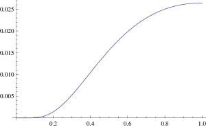
Figure 9: The function $\beta_{10}$.

Figure 10: The function $\beta_{11}$.

5 Thermodynamical stability at first order

In this section we will discuss the thermodynamical stability of our solution. We need to know the temperature of the hairy solution. The temperature of the hairy black hole at first order expressed in terms of the critical temperature is

$$T_{hair}=T_{0}e^{\varepsilon^{2}(-\alpha_{10}(1)+\beta_{10}(1)/2)}~{}.$$ (5.1)

Notice that $T_{hair}\geq T_{0}$, so the RN black hole is unstable at high temperatures (above $T_{0}$) for a fixed charge $Q$. As the mass $M$ approaches its minimum value at extremality, the RN black hole becomes stable.

Since the correction is quadratic in the scalar field, we deduce for the value of the scalar field at the horizon,

$$\varphi_{+}\equiv\varphi\Big{|}_{z=1}=\gamma\sqrt{\frac{T_{hair}}{T_{0}}-1}~{}.$$ (5.2)

Let us find an RN black hole at this temperature. We shall find one with the same charge $Q$. Call the parameters of this black hole $\mu^{\prime}=\mu+\varepsilon^{2}\mu_{1}$ and $B^{\prime}=B+\varepsilon^{2}B_{1}$. Since $\mu/\sinh B=$ const., we have

$$B_{1}=\tanh B\frac{\mu_{1}}{\mu}~{}.$$

Another relation between $B_{1}$ and $\mu_{1}$ is found from setting

$$\frac{\delta T}{T_{0}}=\varepsilon^{2}\left[-\alpha_{10}(1)+\frac{\beta_{10}(1)}{2}\right]~{}.$$

We obtain

$$-\alpha_{10}(1)+\frac{\beta_{0}(1)}{2}=\frac{4}{e^{2B}-1}B_{1}-\frac{\mu_{1}}{\mu}~{}.$$

These two relations determine $B_{1}$ and $\mu_{1}$. For the free energy, we deduce

$$\frac{\delta F_{RN}}{F_{RN}}=\varepsilon^{2}\frac{1+e^{2B}}{3-e^{2B}}\left[-\delta\alpha_{0}(1)+\frac{\beta_{0}(1)}{2}\right]~{}.$$

Notice that $\delta F_{RN}>0$ as long as $e^{2B}<3$.

We need to compare it with the free energy of the hairy black hole. The mass of the hairy black hole is found from the asymptotic behaviour of $\alpha$,

$$GM=\frac{\mu}{2}\alpha_{0}^{\prime}(0)~{},$$

where prime denotes differentiation with respect to $z$. Therefore,

$$GM_{hair}=GM_{RN}+\varepsilon^{2}\frac{\mu}{2}\alpha_{10}^{\prime}(0)~{}.$$

This is found from the surface (Gibbons-Hawking) term in the action. The entropy is found from the area of the horizon,

$$S_{hair}=S_{RN}e^{-\varepsilon^{2}[-\alpha_{10}+\beta_{10}/2]}\Big{|}_{z=1}~{}.$$

Therefore, the product $TS$ remains unchanged.

There is an additional contribution from the Einstein-Hilbert action because the Ricci scalar does not vanish. We obtain a contribution to the free energy

$$\delta F_{EH}=-\int d^{3}x\sqrt{-g}\frac{R}{16\pi G}=-\frac{\varepsilon^{2}}{2}\int d^{3}x\sqrt{-g}(\partial\varphi^{(0)})^{2}~{}.$$

This is the dominant change in the free energy and is clearly negative. Explicitly,

$$\delta F_{EH}=-\frac{2\pi\mu}{3}\int_{0}^{1}\frac{dz}{z^{2}}\varepsilon^{2}\left[(z\mathcal{Z}^{\prime})^{2}+2\mathcal{Z}^{2}\right]<0~{}.$$

Therefore, the difference in free energies is

$$\Delta F=\delta F_{hair}-\delta F_{RN}=\frac{1}{2}\varepsilon^{2}\alpha_{10}^{\prime}(0)F_{RN}-\frac{1+e^{2B}}{3-e^{2B}}\varepsilon^{2}\left[-\alpha_{10}(1)+\frac{\beta_{10}(1)}{2}\right]F_{RN}+\delta F_{EH}~{}~{}.$$ (5.3)

Putting numbers in (5.3) we find $\Delta F=-0.08091$, showing that the hairy black hole is thermodynamically stable.

6 Discussion of the solution

To complete the first-order solution and verify the validity of the perturbative expansion, we determine the first-order correction to the scalar field and calculate various invariants of the metric and show that they are regular at and outside the horizon, showing that no singularity arises at this order.

With our choice of the zeroth-order scalar field $\varphi^{(0)}$ as a dipole (eqs. (3.10) and (3.13)), the first-order correction (eq. (2.9)) contains both a dipole and a $\ell=3$ term. Let

$$\varphi^{(1)}(z,\theta)=\varphi_{10}(z)\cos\theta+\varphi_{11}(z)\cos 3\theta~{}.$$ (6.1)

The field equation obeyed by $\varphi^{(1)}$ is obtained by collecting the first-order terms in the Klein-Gordon equation (2.5). The resulting equation is too long to be included here. It is straightforward to see that it results into decoupled equations for $\varphi_{10}$ and $\varphi_{11}$. The latter involve the functions $\varphi^{(0)}(z),\ \alpha_{10}(z),\ \alpha_{12}(z),\ \beta_{10}(z)$ and $\beta_{11}(z)$, which have already been calculated. Both $\varphi_{10}(z)$ and $\varphi_{11}(z)$ can be seen to behave as $c_{10}z^{2}$ and $c_{11}z^{2}$ in the limit $z\rightarrow 0.$ One may tune the coefficients $c_{10}$ and $c_{11}$ to ensure that the corrections vanish at $z=1.$ The results for the two functions are depicted in figure 11. It is readily seen, upon comparison with figure 2, that the corrections are of the order of the zeroth order contribution, so the series in $\varepsilon$ is expected to have a finite radius of convergence.

Figure 11: The first-order corrections of the scalar field, $\varphi_{10}(z)$ (left panel) and $\varphi_{11}(z)$ (right panel).

Having demonstrated regularity of the first-order corrections to the scalar field, we now turn to addressing the same question regarding the metric. To this end, we need to compute gauge-invariant quantities, such as the Ricci scalar. The Ricci scalar $R$ vanishes at zeroth order since it corresponds to a Reissner-Nordström black hole. We computed $R$ at first order both analytically and numerically and found that it is regular everywhere. In figure 12 we plot $R$ versus $\theta$ for representative values of the radius, namely $z=0.3,\ z=0.6$ and $z=0.9.$ Furthermore, we computed two additional gauge-invariant quantities, $R_{\mu\nu}R^{\mu\nu}$ and $R_{\mu\nu\rho\sigma}R^{\mu\nu\rho\sigma}$ at first-order both analytically and numerically and found them to be regular everywhere (see figure 13). We show the values of the product $R_{\mu\nu}R^{\mu\nu}$ of the Ricci tensors, as well as the product $R_{\mu\nu\rho\sigma}R^{\mu\nu\rho\sigma}$ of the Riemann tensors versus $\theta$ for various values of $z$. We find again that the results are finite and roughly of the same order of magnitude for the three typical values of $z.$

Figure 12: The Ricci scalar $R$ vs. $\theta$ for $z=0.3,\ 0.6,\ 0.9.$ Correspondingly, $R=-0.011,$ $0.0027,$ $0.086$ at $\theta=\frac{\pi}{2}=0.157.$

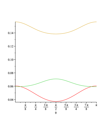
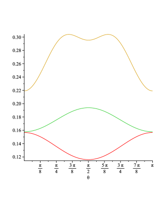
Figure 13: $R_{\mu\nu}R^{\mu\nu}$ (left panel) and $R_{\mu\nu\rho\sigma}R^{\mu\nu\rho\sigma}$ (right panel) vs. $\theta$ for for $z=0.3,\ 0.6,\ 0.9$ (bottom to top).

7 Conclusions

We studied the effect of the presence in the Einstein-Hilbert action of a derivative coupling of a scalar field to Einstein tensor, on static black hole solutions. We considered the Reissner-Nordström black hole solution in isotropic coordinates and in this background we introduced a scalar field coupled to Einstein tensor. For small values of the scalar field we studied in details how the derivative coupling backreacts on the metric, solving the full coupled dynamical system of Einstein-Maxwell-Klein-Gordon equations.

We found that the Reissner-Nordström black hole above a certain critical temperature is destabilized to a new hairy black hole configuration. We studied the properties of this new hairy black hole solution near the critical temperature and we showed that the scalar field is regular on the horizon and at infinity. The no-hair theorem is evaded due to the presence of the derivative coupling of the scalar field to the Einstein tensor. This new “Einstein hair” solution is in general anisotropic with the scalar field and the metric functions to depend also on the angular coordinate. We calculated the mass and the temperature of the new hairy black hole solution and by considering the free energies we showed that the new hairy black hole configuration is thermodynamically stable.

It would be interesting to extend the analysis to more general “Einstein hair” by including mass and charge for the scalar hair and explore the existence of spherically symmetric hair. In particular, it would be of great interest to see if hair can develop down to zero temperature and form a configuration of vanishing entropy. Work in this direction is in progress.

Appendix A First-order solution of Einstein-Maxwell equations

In this appendix we give the technical details of solving the field equations (2.15)-(2.19) at first order in the order parameter $\varepsilon^{2}$. We start with (2.15). On the right-hand side, only $\varphi^{(0)}$ contributes and only through $\Theta_{\mu\nu}$. Using (4.1), we obtain

$$z^{2}\partial_{z}^{2}l-z\partial_{z}l+\partial_{\theta}^{2}l+2\cot\theta\partial_{\theta}l=8\pi G\frac{\mu^{2}\kappa}{z^{2}}l_{0}^{3}e^{\alpha}(-\Theta_{t}^{t}-\Theta_{\phi}^{\phi})+\mathcal{O}(\varepsilon^{4})=\mathcal{O}(\varepsilon^{4})~{},$$ (A.1)

which has as a solution

$$l=1-z^{2}+\mathcal{O}(\varepsilon^{4})~{},$$ (A.2)

therefore $l$ is unchanged at first order, $l_{1}=0$ (recall eqs. (3.3) and (3.9) for an RN black hole).

Next we solve the Maxwell equation which takes the explicit form

$$z^{2}\partial_{z}^{2}A+z^{2}\partial_{z}(\alpha+\ln l)\partial_{z}A+\partial_{\theta}^{2}A+\left[\cot\theta+\partial_{\theta}\alpha+\partial_{\theta}\ln l\right]\partial_{\theta}A=0~{}.$$ (A.3)

At first order,

$$z^{2}\partial_{z}^{2}A+\left[-\frac{2z}{l}+\partial_{z}\alpha\right]z^{2}\partial_{z}A+\partial_{\theta}^{2}A+\cot\theta\partial_{\theta}A=\mathcal{O}(\varepsilon^{4})~{}.$$ (A.4)

From (2.16), at first order we have

$$z^{2}\partial_{z}^{2}\alpha-\frac{2z^{3}}{l}\partial_{z}\alpha+\partial_{\theta}^{2}\alpha+\cot\theta\partial_{\theta}\alpha=8\pi Ge^{\alpha}\left[(z\partial_{z}A)^{2}+2\mu^{2}\kappa\frac{l^{2}}{z^{2}}\Theta_{t}^{t}\right]+\mathcal{O}(\varepsilon^{4})~{}.$$

We expand the first-order corrections in Legendre polynomials,

$$\alpha_{1} = \alpha_{10}(z)P_{0}(\cos\theta)+\alpha_{12}(z)P_{2}(\cos\theta)~{},$$

$$A_{1} = A_{10}(z)P_{0}(\cos\theta)+A_{12}(z)P_{2}(\cos\theta)~{},$$

$$\mu^{2}\frac{l^{2}}{z^{2}}e^{\alpha}\Theta_{t}^{t} = \varepsilon^{2}[\mathcal{Q}_{0}(z)P_{0}(\cos\theta)+\mathcal{Q}_{2}(z)P_{2}(\cos\theta)]+\mathcal{O}(\varepsilon^{4})~{},$$ (A.5)

where

$$\mathcal{Q}_{0}=\frac{\mathcal{R}}{6}\left[\frac{1}{2}(z\mathcal{Z}^{\prime})^{2}+\mathcal{Z}^{2}\right]~{},\ \ \ \ \mathcal{Q}_{2}=\frac{\mathcal{R}}{6}\left[(z\mathcal{Z}^{\prime})^{2}-\mathcal{Z}^{2}\right]~{},$$ (A.6)

and $\mathcal{R}$ is given in (3.12).

Using

$$P_{\ell}^{\prime\prime}(\cos\theta)+\cot\theta P_{\ell}^{\prime}(\cos\theta)=-\ell(\ell+1)P_{\ell}(\cos\theta)~{},$$

we obtain

$$(A_{0}+\varepsilon^{2}A_{10})^{\prime\prime}+\left[-\frac{2z}{l}+(\alpha_{0}+\varepsilon\alpha_{10})^{\prime}\right](A_{0}+\varepsilon^{2}A_{10})^{\prime} = \mathcal{O}(\varepsilon^{4})~{},$$ (A.7)

$$A_{2}^{\prime\prime}+\left[-\frac{2z}{l_{0}}+\alpha_{0}^{\prime}\right]A_{2}^{\prime}-\frac{6}{z^{2}}A_{2} = -\alpha_{2}^{\prime}A_{0}^{\prime}~{},$$ (A.8)

$$(\alpha_{0}+\varepsilon^{2}\alpha_{10})^{\prime\prime}-\frac{2z}{l}(\alpha_{0}+\varepsilon^{2}\alpha_{10})^{\prime}-8\pi Ge^{\alpha_{0}+\varepsilon^{2}\alpha_{10}}{(A_{0}+\varepsilon^{2}A_{10})^{\prime}}^{2} = 16\pi G\kappa\frac{\varepsilon^{2}\mathcal{Q}_{0}}{z^{2}}+\mathcal{O}(\varepsilon^{4})~{},$$

$$\alpha_{12}^{\prime\prime}-\frac{2z}{l_{0}}\alpha_{12}^{\prime}-\frac{6}{z^{2}}\alpha_{12}-8\pi Ge^{\alpha_{0}}{A_{0}^{\prime}}^{2}\alpha_{12}-16\pi Ge^{\alpha_{0}}A_{0}^{\prime}A_{2}^{\prime} = 16\pi G\kappa\frac{\mathcal{Q}_{2}}{z^{2}}~{}.$$ (A.10)

From (A.7) we deduce

$$A_{0}(z)+\varepsilon^{2}A_{10}(z)=\frac{Q}{\mu}\int_{z}^{1}\frac{dz^{\prime}}{l(z^{\prime})}e^{-\alpha_{0}(z^{\prime})-\varepsilon^{2}\alpha_{10}(z^{\prime})}+\mathcal{O}(\varepsilon^{4})~{}.$$ (A.11)

Eq. (LABEL:eqx3) implies that the angle-independent part of first-order correction of $\alpha$ satisfies

$$\alpha_{10}^{\prime\prime}-\frac{2z}{1-z^{2}}\alpha_{10}^{\prime}-\frac{8}{[(1+z^{2})\sinh B+2z\cosh B]^{2}}\alpha_{10}=16\pi G\frac{\kappa\mathcal{Q}_{0}}{z^{2}}~{}.$$ (A.12)

To solve it, first we look at the boundary conditions. At the boundary, $\alpha_{10}^{\prime\prime}\approx 0$, therefore

$$\alpha_{10}\sim\lambda z~{}.$$ (A.13)

At the horizon, $(1-z)\alpha_{10}^{\prime\prime}-\alpha_{10}^{\prime}\approx 0$, therefore $\alpha_{10}\sim$const., or $\alpha_{10}\sim\ln(1-z)$. The solution that asymptotes to $\lambda z$ as $z\to 0$ yields a mixture $\alpha_{10}\sim a+b\ln(1-z)$ at the horizon. There is a unique value of $\lambda$ for which $b=0$ and the solution is regular.

The remaining two equations form a coupled system to be solved for the angle-dependent first-order contributions $A_{12}$ and $\alpha_{12}$. Explicitly,

$$A_{12}^{\prime\prime}-\frac{2}{z}\left[\frac{l_{0}}{1+z^{2}+2z\coth B}-\frac{1}{l_{0}}\right]A_{12}^{\prime}-\frac{6}{z^{2}}A_{12} = -\frac{Q}{\mu}\frac{l_{0}}{(1+z^{2}+2z\coth B)^{2}}\alpha_{12}^{\prime}~{},$$

$$\alpha_{12}^{\prime\prime}-\frac{2z}{l_{0}}\alpha_{12}^{\prime}-\left[\frac{6}{z^{2}}+\frac{8}{[(1+z^{2})\sinh B+2z\cosh B]^{2}}\right]\alpha_{12} = -\frac{16\pi GQ}{\mu}\frac{1}{l_{0}}A_{12}^{\prime}+16\pi G\frac{\kappa\mathcal{Q}_{2}}{z^{2}}~{}.$$

As $z\to 0$, we have

$$A_{12}=\mathcal{A}z^{3}+\dots\ ,\ \ \alpha_{12}=\mathbf{a}z^{3}+\dots$$ (A.16)

The constants $\mathcal{A}$ and $\mathbf{a}$ are fixed by demanding $\alpha_{12}=A_{12}=0$ at the horizon (so there is no angular dependence of the temperature or an electric field along the horizon).

Finally, we obtain $\beta$ from the third Einstein equation (2.17). At zeroth order, we have

$$0=-\frac{1}{2}(z\alpha_{0}^{\prime})^{2}-3\frac{zl_{0}^{\prime}}{l_{0}}+2\left(\frac{zl_{0}^{\prime}}{l_{0}}\right)^{2}-\frac{z^{2}l_{0}^{\prime\prime}}{l_{0}}+8\pi Ge^{\alpha_{0}}(zA_{0}^{\prime})^{2}~{},$$ (A.17)

which is easily seen to be satisfied.

To solve the equation at first order, we set

$$\beta_{1}=\beta_{10}(z)+\beta_{11}(z)\cos^{2}\theta~{}.$$ (A.18)

and obtain

$$(1+z^{2})z\beta_{10}^{\prime}=\mathcal{S}_{0}(z)~{},$$ (A.19)

where

$$\mathcal{S}_{0}(z) = \frac{4z^{2}[(1+z^{2})\cosh B+2z\sinh B]}{(1+z^{2})\sinh B+2z\cosh B}\left(\alpha_{10}^{\prime}-\frac{1}{2}\alpha_{12}^{\prime}\right)$$ (A.20)

$$- \frac{8z^{2}(1-z^{2})}{[(1+z^{2})\sinh B+2z\cosh B]^{2}}\left(\alpha_{10}-\frac{1}{2}\alpha_{12}\right)$$

$$- 8\pi G(1-z^{2})\left[1-\frac{4\kappa z^{4}}{\mu^{2}[(1+z^{2})\sinh B+2z\cosh B]^{4}}\right]\mathcal{Z}^{2}~{}.$$

to be solved for $\beta_{10}(z)$, and

$$(1+z^{2})z\beta_{11}^{\prime}-2(1-z^{2})\beta_{11}=\mathcal{S}_{1}(z)~{},$$ (A.21)

where

$$\mathcal{S}_{1}(z) = \frac{12z^{2}[(1+z^{2})\cosh B+2z\sinh B]}{(1+z^{2})\sinh B+2z\cosh B}\alpha_{12}^{\prime}+\frac{12z^{2}(1-z^{2})}{[(1+z^{2})\sinh B+2z\cosh B]^{2}}\alpha_{12}$$

$$+ 8\pi G(1-z^{2})[(z\mathcal{Z}^{\prime})^{2}+\mathcal{Z}^{2}]+8\pi G\frac{4\kappa z^{4}(1-z^{2})}{\mu^{2}[(1+z^{2})\sinh B+2z\cosh B]^{4}}[(z\mathcal{Z}^{\prime})^{2}-\mathcal{Z}^{2}]~{},$$

to be solved for $\beta_{11}(z)$.

They are both first-order equations and are easily integrated. We obtain

$$\beta_{10}(z)=\int_{0}^{z}\frac{dy}{y(1+y^{2})}\,\mathcal{S}_{0}(y)$$ (A.23)

where we used the boundary condition $\beta_{10}(0)=0$.

For $\beta_{11}$, we need $\beta_{11}=0$ at both ends. We obtain

$$\beta_{11}=-\frac{z^{2}}{(1+z^{2})^{2}}\int_{z}^{1}\frac{dy}{y^{3}}(1+y^{2})\mathcal{S}_{1}(y)$$ (A.24)

where the limit of integration was chosen so that $\beta_{11}=0$ at the horizon ($z=1$). Notice that $\beta_{11}\sim\mathcal{O}(z^{2})$ as $z\to 0$ ($r\to\infty$), so the other boundary condition is also satisfied.

References

-
[1]
J. E. Chase, “Event horizons in static scalar-vacuum space-times,”
Commun. Math. Phys. 19, 276 (1970);
J. D. Bekenstein, “Transcendence of the Law of Baryon-Number Conservation in Black-Hole Physics,” Phys. Rev. Lett. 28, 452 (1972);
2403 (1972);
M. Heusler, “A Mass Bound for Spherically Symmetric Black Hole Spacetimes,” Class. Quant. Grav. 12, 779 (1995) [arXiv:gr-qc/9411054];
M. Heusler and N. Straumann, “Scaling arguments for the existence of static, spherically symmetric solutions of self-gravitating systems,” Class. Quant. Grav. 9, 2177 (1992);
D. Sudarsky, “A simple proof of a no-hair theorem in Einstein-Higgs theory,” Class. Quant. Grav. 12, 579 (1995);
J. D. Bekenstein, “Novel ‘no-scalar-hair’ theorem for black holes,” Phys. Rev. D 51, R6608 (1995). -
[2]
A. E. Mayo and J. D. Bekenstein,
“No hair for spherical black holes: charged and nonminimally coupled scalar
field with self–interaction,”
Phys. Rev. D 54, 5059 (1996)
[arXiv:gr-qc/9602057];
J. D. Bekenstein, “Black hole hair: Twenty-five years after,” arXiv:gr-qc/9605059. -
[3]
N. Bocharova, K. Bronnikov and V. Melnikov, Vestn. Mosk.
Univ. Fiz. Astron. 6, 706 (1970);
J. D. Bekenstein, Annals Phys. 82, 535 (1974);
J. D. Bekenstein, “Black Holes With Scalar Charge,” Annals Phys. 91, 75 (1975). - [4] K. A. Bronnikov and Y. N. Kireyev, “Instability of black holes with scalar charge,” Phys. Lett. A 67, 95 (1978).
- [5] K. G. Zloshchastiev, “On co-existence of black holes and scalar field,” Phys. Rev. Lett. 94, 121101 (2005) [arXiv:hep-th/0408163].
- [6] T. Torii, K. Maeda and M. Narita, “No-scalar hair conjecture in asymptotic de Sitter spacetime,” Phys. Rev. D 59, 064027 (1999) [arXiv:gr-qc/9809036].
- [7] C. Martinez, R. Troncoso and J. Zanelli, “de Sitter black hole with a conformally coupled scalar field in four dimensions,” Phys. Rev. D 67, 024008 (2003) [arXiv:hep-th/0205319].
- [8] T. J. T. Harper, P. A. Thomas, E. Winstanley and P. M. Young, “Instability of a four-dimensional de Sitter black hole with a conformally coupled scalar field,” Phys. Rev. D 70, 064023 (2004) [arXiv:gr-qc/0312104].
- [9] G. Dotti, R. J. Gleiser and C. Martinez, “Static black hole solutions with a self interacting conformally coupled scalar field,” Phys. Rev. D 77, 104035 (2008) [arXiv:0710.1735 [hep-th]].
- [10] T. Torii, K. Maeda and M. Narita, “Scalar hair on the black hole in asymptotically anti-de Sitter spacetime,” Phys. Rev. D 64, 044007 (2001).
- [11] E. Winstanley, “On the existence of conformally coupled scalar field hair for black holes in (anti-)de Sitter space,” Found. Phys. 33, 111 (2003) [arXiv:gr-qc/0205092].
- [12] C. Martinez, R. Troncoso and J. Zanelli, “Exact black hole solution with a minimally coupled scalar field,” Phys. Rev. D 70, 084035 (2004) [arXiv:hep-th/0406111].
-
[13]
C. Martinez, J. P. Staforelli and R. Troncoso,
“Topological black holes dressed with a conformally coupled scalar field and
electric charge,”
Phys. Rev. D 74, 044028 (2006)
[arXiv:hep-th/0512022];
C. Martinez and R. Troncoso, “Electrically charged black hole with scalar hair,” Phys. Rev. D 74, 064007 (2006) [arXiv:hep-th/0606130]. - [14] T. Kolyvaris, G. Koutsoumbas, E. Papantonopoulos and G. Siopsis, “A New Class of Exact Hairy Black Hole Solutions,” Gen. Rel. Grav. 43, 163 (2011) [arXiv:0911.1711 [hep-th]].
- [15] G. Koutsoumbas, E. Papantonopoulos and G. Siopsis, “Exact Gravity Dual of a Gapless Superconductor,” JHEP 0907, 026 (2009) [arXiv:0902.0733 [hep-th]].
-
[16]
G. Koutsoumbas, S. Musiri, E. Papantonopoulos and G. Siopsis,
“Quasi-normal modes of electromagnetic perturbations of four-dimensional
topological black holes with scalar hair,”
JHEP 0610, 006 (2006)
[arXiv:hep-th/0606096];
G. Koutsoumbas, E. Papantonopoulos and G. Siopsis, “Phase Transitions in Charged Topological-AdS Black Holes,” JHEP 0805, 107 (2008) [arXiv:0801.4921 [hep-th]];
G. Koutsoumbas, E. Papantonopoulos and G. Siopsis, “Discontinuities in Scalar Perturbations of Topological Black Holes,” Class. Quant. Grav. 26, 105004 (2009) [arXiv:0806.1452 [hep-th]]. - [17] C. Charmousis, T. Kolyvaris and E. Papantonopoulos, “Charged C-metric with conformally coupled scalar field,” Class. Quant. Grav. 26, 175012 (2009) [arXiv:0906.5568 [gr-qc]].
- [18] A. Anabalon and H. Maeda, “New Charged Black Holes with Conformal Scalar Hair,” arXiv:0907.0219 [hep-th].
- [19] K. Farakos, A. P. Kouretsis and P. Pasipoularides, “Anti de Sitter 5D black hole solutions with a self-interacting bulk scalar field: a potential reconstruction approach,” Phys. Rev. D 80, 064020 (2009) [arXiv:0905.1345 [hep-th]].
- [20] N. Ohta and T. Torii, “Black Holes in the Dilatonic Einstein-Gauss-Bonnet Theory in Various Dimensions IV - Topological Black Holes with and without Cosmological Term,” arXiv:0908.3918 [hep-th].
- [21] L. Amendola, “Cosmology with nonminimal derivative couplings,” Phys. Lett. B 301, 175 (1993) [arXiv:gr-qc/9302010].
- [22] S. V. Sushkov, “Exact cosmological solutions with nonminimal derivative coupling,” Phys. Rev. D 80, 103505 (2009) [arXiv:0910.0980 [gr-qc]].
- [23] C. Gao, “When scalar field is kinetically coupled to the Einstein tensor,” JCAP 1006, 023 (2010) [arXiv:1002.4035 [gr-qc]].
- [24] L. N. Granda, “Non-minimal Kinetic coupling to gravity and accelerated expansion,” JCAP 1007, 006 (2010) [arXiv:0911.3702 [hep-th]].
- [25] E. N. Saridakis and S. V. Sushkov, “Quintessence and phantom cosmology with non-minimal derivative coupling,” Phys. Rev. D 81, 083510 (2010) [arXiv:1002.3478 [gr-qc]].
- [26] C. Germani, A. Kehagias, “New Model of Inflation with Non-minimal Derivative Coupling of Standard Model Higgs Boson to Gravity,” Phys. Rev. Lett. 105, 011302 (2010). [arXiv:1003.2635 [hep-ph]].
- [27] C. Germani, L. Martucci and P. Moyassari, “Introducing the Slotheon: a slow Galileon scalar field in curved space-time,” Phys. Rev. D 85, 103501 (2012) [arXiv:1108.1406 [hep-th]].
- [28] S. Chen and J. Jing, “Dynamical evolution of a scalar field coupling to Einstein’s tensor in the Reissner-Nordström black hole spacetime,” Phys. Rev. D 82, 084006 (2010) [arXiv:1007.2019 [gr-qc]].
- [29] B. Kleihaus and J. Kunz, “Static axially symmetric Einstein Yang-Mills dilaton solutions. 2. Black hole solutions,” Phys. Rev. D 57, 6138 (1998) [arXiv:gr-qc/9712086].