Extended Lagrangian free energy molecular dynamics

Abstract

Extended free energy Lagrangians are proposed for first principles molecular dynamics simulations at finite electronic temperatures for plane-wave pseudopotential and local orbital density matrix based calculations. Thanks to the extended Lagrangian description the electronic degrees of freedom can be integrated by stable geometric schemes that conserve the free energy. For the local orbital representations both the nuclear and electronic forces have simple and numerically efficient expressions that are well suited for reduced complexity calculations. A rapidly converging recursive Fermi operator expansion method that does not require the calculation of eigenvalues and eigenfunctions for the construction of the fractionally occupied density matrix is discussed. An efficient expression for the Pulay force that is valid also for density matrices with fractional occupation occurring at finite electronic temperatures is also demonstrated.

I Introduction

Molecular dynamics simulations are widely used in materials science, chemistry and molecular biology. Unfortunately, the most accurate molecular dynamics methods that are based on self-consistent field (SCF) theory Marx and Hutter (2000) are often limited by some fundamental shortcomings such as a very high computational cost or unbalanced phase space trajectories with unphysical hysteresis effects, numerical instabilities and a systematic long-term energy drift Pulay and Fogarasi (2004); Niklasson et al. (2006). Recently an extended Lagrangian framework for first principles molecular dynamics simulations was proposed that overcomes most of the previous problems Niklasson (2008a). The new framework was originally designed for ground state Born-Oppenheimer molecular dynamics simulations based on Hartree-Fock Roothaan (1951) or density functional theory Hohenberg and Kohn (1964); Kohn and Sham (1965) at zero electronic temperatures. In this paper we supplement previous work by proposing extended free energy Lagrangians for first principles molecular dynamics simulations also at finite electronic temperatures Mermin (1965); Parr and Yang (1989).

Our extended Lagrangian free energy dynamics is formulated and demonstrated both for plane-wave pseudopotential and local orbital density matrix based calculations. For the density matrix formulation our approach is given by a generalization of the original extended Lagrangian framework Niklasson (2008a) using a density matrix representation of the electronic degrees of freedom with fractional occupation of the states. The plane-wave formulation is based on the wave function extended Lagrangian molecular dynamics method that recently was proposed by Steneteg et al. Steneteg et al. (2010).

First we formulate the extended Lagrangian approach to first principles molecular dynamics at finite electronic temperatures for local orbital density matrix representations and thereafter for plane wave pseudopotential calculations. A numerically efficient expression for a generalized Pulay force that does not require idempotent density matrices is demonstrated and a recursive Fermi operator expansion algorithm for the density matrix is discussed. Thereafter a Verlet integration scheme for the equations of motion is presented. Finally, we illustrate the extended Lagrangian free energy dynamics by some examples before giving a brief summary.

II First principles molecular dynamics at finite electronic temperatures

The first principles molecular dynamics scheme presented in this paper is a finite electronic temperature generalization of the extended Lagrangian framework of time-reversible Born-Oppenheimer molecular dynamics Niklasson et al. (2006); Niklasson (2008a). In many ways the generalization is straightforward, except for an additional entropy term, problems arising in the construction of the density matrix, the calculation of the Pulay force for fractional occupations and the phase alignment problem in the integration of the wave functions Steneteg et al. (2010). Our two different formulations of extended Lagrangian free energy molecular dynamics are based on either an underlying local orbital representation or a plane wave pseudo potential description. Alternative free energy formulations suitable for extended Lagrangian self-consistent tight-binding molecular dynamics simulations Sanville et al. (2010); Zheng et al. (2011) will be presented elsewhere.

II.1 Density matrix extended free energy Lagrangian

Within an atom-centered local orbital representation we describe our first principles molecular dynamics at an electronic temperature, $T_{e}$, by a density matrix (DM) extended free energy (XFE) Lagrangian, which we define as

$$\begin{array}[]{l}{\cal L}^{\rm XFE}_{\rm DM}({\bf R},{\bf\dot{R}},P,{\dot{P}})=\frac{1}{2}\sum_{k}M_{k}{\dot{R}}_{k}^{2}-U[{\bf R};D]\\ {}\\ ~{}~{}~{}~{}+\frac{1}{2}\mu\mathrm{Tr}[{\dot{P}}^{2}]-\frac{1}{2}\mu\omega^{2}\mathrm{Tr}[(D-P)^{2}]+T_{e}{\cal S}[D].\end{array}$$ (1)

The extended dynamical variables $P$ and the velocity ${\dot{P}}$ in the Lagrangian ${\cal L}^{\rm XFE}_{\rm DM}$ are auxiliary electronic degrees of freedom evolving in a harmonic potential centered around the self-consistent free energy ground-state solution $D$ Niklasson (2008a). Here $P$, ${\dot{P}}$, and the self-consistent free energy ground state $D$, are orthogonal density matrix representations of the electronic degrees of freedom. The relation between $D$ and the non-orthogonal (atomic orbital) representation, ${\widetilde{D}}$, is given by the congruence transformation

$${\widetilde{D}}=ZDZ^{T},$$ (2)

where $Z$ is a congruence factor determined by the overlap matrix $S$ (e.g. see Ref. Niklasson and Weber (2007)) from the condition that

$$Z^{T}SZ=I.$$ (3)

The constants $\mu$ and $\omega$ are fictitious electron mass and frequency parameters. The potential $U[{\bf R};D]$ is defined at the self-consistent field (SCF) electron ground state $D$, at which the free energy functional

$$\Omega[{\bf R},D]=U[{\bf R};D]-T_{e}{\cal S}[D],$$ (4)

has its minimum for a given nuclear configuration, ${\bf R}=\{R_{i}\}$, Mermin (1965); Parr and Yang (1989) under the constraints of correct electron occupation, $\mathrm{Tr}[D]=N_{\rm occ}$. The electronic temperature $T_{e}$ can be different from the ionic temperature $T_{\rm ion}$. We assume that $U[{\bf R};D]$ is the total electronic energy, including nuclear ion-ion repulsions, in self-consistent density functional theory, Hartree-Fock theory or some of their extensions that are based on an underlying SCF description. The mean field entropy term in ${\cal L}^{\rm XFE}$,

$${\cal S}[D]=-2k_{B}\mathrm{Tr}[D\ln(D)+(I-D)\ln(I-D)],$$ (5)

is included to provide the variationally correct energetics and dynamics Weinert and Davenport (1992); Wentzcovitch et al. (1992). The factor 2 above is used for restricted calculations (not spin polarized) when each state is doubly occupied, which is assumed throughout the paper.

II.1.1 Euler-Lagrange equations of motion

The time evolution of the system described by ${\cal L}^{\rm XFE}_{\rm DM}$ is determined by the Euler-Lagrange equations,

$$\frac{d}{dt}\left(\frac{\partial{\cal L}^{\rm XFE}_{\rm DM}}{\partial{\dot{R}}_{k}}\right) = \frac{\partial{\cal L}^{\rm XFE}_{\rm DM}}{\partial{R}_{k}},$$ (6)

$$\frac{d}{dt}\left(\frac{\partial{\cal L}^{\rm XFE}_{\rm DM}}{\partial{\dot{P}}}\right) = \frac{\partial{\cal L}^{\rm XFE}_{\rm DM}}{\partial P},$$ (7)

which give the equations of motion for the nuclear and electronic degrees of freedom,

$$M_{k}{\ddot{R}}_{k} = -\frac{\partial U\left[{\bf R};D\right]}{\partial R_{k}}+T\frac{\partial{\cal S}[D]}{\partial R_{k}}-\frac{\mu\omega^{2}}{2}\frac{\partial\mathrm{Tr}[(D-P)^{2}]}{\partial R_{k}},$$

$$\mu{\ddot{P}} = \mu{\omega^{2}}(D-P).$$ (9)

In the limit $\mu\rightarrow 0$, we get the decoupled equations

$$M_{k}{\ddot{R}}_{k} = -\frac{\partial U\left[{\bf R};D\right]}{\partial R_{k}}+T_{e}\frac{\partial{\cal S}[D]}{\partial R_{k}},$$ (10)

$${\ddot{P}} = {\omega^{2}}(D-P),$$ (11)

where the self-consistent density matrix $D$ is given from the Fermi operator expansion

$$D=\left[e^{\beta(H-\mu_{0}I)}+I\right]^{-1},$$ (12)

under the canonical condition of charge neutrality,

$$\mathrm{Tr}[D]=\mathrm{Tr}[{\widetilde{D}}S]=N_{\rm occ.},$$ (13)

i.e. the chemical potential $\mu_{0}$ is set such that the trace of $D$ is the number of occupied states. The inverse temperature $\beta=1/(k_{B}T_{e})$. The orthogonalized effective single-particle Hamiltonian $H$, i.e. the Fockian or Kohn-Sham Hamiltonian, is given by a congruence transformation of the Fockian in a non-orthogonal (atomic orbital) representation, ${\widetilde{H}}$, where

$$H=Z^{T}{\widetilde{H}}Z.$$ (14)

Since we use the limit $\mu\rightarrow 0$, we recover the regular free energy Lagrangain (without extention) and the total free energy is a constant of motion that is unaffected by the extended variables $P$ and ${\dot{P}}$. This is in contrast to extended Lagrangian Car-Parrinello type molecular dynamics Car and Parrinello (1985); Hartke and Carter (1992); Schlegel et al. (2001); Herbert and Head-Gordon (2004). The major advantage of the auxiliary set of variables $P$ and ${\dot{P}}$ occurs in the SCF optimization and in the geometric integration of the equations of motion discussed in section III below.

II.2 Wave Function Extended Free Energy Lagrangian

In plane wave (PW) pseudopotential methods it is convenient to propagate both the electronic wave functions, $\Phi=\{\phi_{m}({\bf r})\}$, and the density, $\rho({\bf r})$. In this case we define the wave function (and density) extended free energy Lagrangian Steneteg et al. (2010) as

$$\begin{array}[]{l}{\cal L}^{\rm XFE}_{\rm PW}({\bf R},{\bf\dot{R}},\Phi,{\dot{\Phi}},\rho,{\dot{\rho}})=\frac{1}{2}\sum_{k}M_{k}{\dot{R}}_{k}^{2}-U[{\bf R};n^{\rm sc}]\\ {}\\ +\frac{1}{2}\mu\sum_{m}\int|{\dot{\phi}}_{m}({\bf r})|^{2}d{\bf r}-\frac{1}{2}\mu\omega^{2}\sum_{m}\int|\psi^{sc}_{m}({\bf r})-\phi_{m}({\bf r})|^{2}d{\bf r}\\ {}\\ +\frac{1}{2}\mu\int|{\dot{\rho}({\bf r})}|^{2}d{\bf r}-\frac{1}{2}\mu\omega^{2}\int|n^{sc}({\bf r})-\rho({\bf r})|^{2}d{\bf r}+T_{e}{\cal S}[{\bf f}].\end{array}$$ (15)

The auxiliary electronic degrees of freedom $\Phi$ and $\rho$ are extended through harmonic oscillators centered around the self-consistent (sc) ground state wave functions $\Psi^{\rm sc}=\{\Psi_{m}({\bf r})\}$ and densities $n^{\rm sc}$. As above, $\mu$ is a fictitious electron mass parameter and $\omega$ is a frequency parameter determining the curvature of the harmonic potentials. As for the density matrix extension, the potential $U[{\bf R};n^{\rm sc}]$ is defined at the self-consistent field (SCF) electron ground state $n^{\rm sc}$, at which the free energy functional

$$\Omega[{\bf R},n^{\rm sc}]=U[{\bf R};n^{\rm sc}]-T_{e}{\cal S}[{\bf f}],$$ (16)

has its minimum for a given nuclear configuration, ${\bf R}=\{R_{i}\}$, Mermin (1965); Parr and Yang (1989) under the constraints of correct electron occupation, $\int n^{sc}({\bf r})d{\bf r}=N_{\rm occ}$. The mean field entropy term in ${\cal L}^{\rm XFE}_{\rm PW}$ is given analogous to Eq. (5) as a function of the occupation numbers, ${\bf f}=\{f_{i}\}$, where

$${\cal S}[{\bf f}]=-2k_{B}\sum_{i}\left(f_{i}\ln(f_{i})+(1-f_{i})\ln(1-f_{i})\right),$$ (17)

and

$$f_{i}=\left[e^{\beta(\varepsilon_{i}-\mu_{0})}+1\right]^{-1}.$$ (18)

Here $\varepsilon_{i}$ are the eigenvalues of the effective single particle (Kohn-Sham) Hamiltonian, i.e.

$$H\psi_{i}=\varepsilon_{i}\psi_{i}.$$ (19)

The entropy term ${\cal S}[{\bf f}]$ provides a variationally correct energetics and dynamics Weinert and Davenport (1992); Wentzcovitch et al. (1992) where the electron density is given by

$$n^{\rm sc}({\bf r})=\sum_{m}\int f_{m}|\psi^{\rm sc}_{m}({\bf r})|^{2}d{\bf r}.$$ (20)

II.2.1 Euler-Lagrange equations of motion

As for the density matrix extended free energy Lagrangian, the dynamics for the wave function extended free energy Lagrangian is determined by the Euler-Lagrange equations, which give the equations of motion for the nuclear and electronic degrees of freedom,

$$M_{k}{\ddot{R}}_{k}=-\frac{\partial U\left[{\bf R};n^{\rm sc}\right]}{\partial R_{k}}+$$ (21)

$$~{}~{}{}-\frac{\mu\omega^{2}}{2}\frac{\partial}{\partial R_{k}}\left(\sum_{n}\int|\psi^{sc}_{n}-\phi_{n}|^{2}d{\bf r}\right)$$

$$~{}~{}{}-\frac{\mu\omega^{2}}{2}\frac{\partial}{\partial R_{k}}\left(\int|n^{\rm sc}({\bf r})-\rho({\bf r})|^{2}d{\bf r}\right)+T_{e}\frac{\partial{\cal S}[{\bf f}]}{\partial R_{k}},$$

$$\mu{\ddot{\Phi}}=\mu{\omega^{2}}(\Psi^{\rm sc}-\Phi),$$ (22)

$$\mu{\ddot{\rho}}({\bf r})=\mu{\omega^{2}}(n^{\rm sc}({\bf r})-\rho({\bf r})).$$ (23)

In the limit $\mu\rightarrow 0$, we get the decoupled equations

$$M_{k}{\ddot{R}}_{k} = -\frac{\partial U\left[{\bf R};n^{\rm sc}\right]}{\partial R_{k}}+T_{e}\frac{\partial{\cal S}[{\bf f}]}{\partial R_{k}},$$ (24)

$${\ddot{\Psi}} = {\omega^{2}}(\Psi^{\rm sc}-\Phi),$$ (25)

$${\ddot{\rho}}({\bf r}) = {\omega^{2}}(n^{\rm sc}({\bf r})-\rho({\bf r})).$$ (26)

Also in this case, the total free energy is a constant of motion in the limit $\mu\rightarrow 0$. The advantages with the extended equations of motion occur in the SCF optimization and geometric integration discussed in section III.

II.3 Generalized Pulay force

The nuclear force ${\cal F}^{\rm tot}=M_{k}{\ddot{R}}_{k}$ in Eqs. (10) and (24) can be partitioned into three separate terms,

$${\cal F}^{\rm tot}={\cal F}^{\rm HF}+{\cal F}^{\rm P}+{\cal F^{S}}.$$ (27)

The first term, ${\cal F}^{\rm HF}$, is the Hellmann-Feynman force term Pulay (1969); Schlegel (2000) for a fractional occupation of the states Weinert and Davenport (1992); Wentzcovitch et al. (1992) (including nuclear-nuclear repulsion). The second term, ${\cal F}^{\rm P}$, corresponds to the Pulay force term Pulay (1969), and the third term,

$${\cal F^{S}}_{k}=T_{e}({\partial}{\cal S}/{\partial R_{k}}),$$ (28)

is an additional entropy force term.

In a plane wave formulation the Pulay force term usually vanishes, but only at $T_{e}=0$. At finite electronic temperatures the Pulay term is finite even for a constant plane wave basis set representation. In this case however, the Pulay term is exactly cancelled by the entropy force term ${\cal F^{S}}$ if the entropy is given by Eq. (17). This is not true for a local orbital basis set representation. In this case only a part of the Pulay force term ${\cal F}^{\rm P}$ is canceled by the entropy contribution ${\cal F^{S}}$ Niklasson (2008b). Nevertheless, this cancellation provides a significant simplification of the Pulay term. The remaining force term can be viewed as a generalized ($G$) Pulay force Niklasson (2008b),

$${\cal F}^{\rm P}_{G}={\cal F}^{\rm P}+{\cal F^{S}}=2\mathrm{Tr}[S^{-1}{\widetilde{H}}{\widetilde{D}}(\partial S/\partial R_{k})],$$ (29)

which is valid for finite temperature ensembles with non-integer occupation Niklasson (2008b). For a constant orthonormal plane wave basis set representation the overlap matrix is equal to the identity matrix, i.e. $S=I$, and the generalized Pulay term disappears. A similar convenient expression for the Pulay force term was recently given by Schlegel et al. Schlegel et al. (2001), but without considering any entropy contribution from fractional occupation. A generalized Pulay force was also discussed in connection to the efficient Ehrenfest-like molecular dynamics scheme by Jakowski and Morokuma Jakowski and Morokuma (2009). In the present formulation the electronic entropy is necessary to make our free energy and forces variationally correct in a molecular dynamics simulation with factional occupation of the states at finite electronic temperatures Weinert and Davenport (1992); Wentzcovitch et al. (1992). The density matrix or the density that minimizes the free energy functional in Eq. (4) or in Eq. (16) with the particular form of the entropy term in Eq. (5) or in Eq. (17) are given by the Fermi operator expansion in Eq. (12) or by Fermi weighted integration in Eq. (20). If other expressions of the entropy are used, the Pulay force expression in Eq. (29) may still be valid Warren and Dunlap (1996), but the density matrix $D$ and wave functions will have a fractional occupation distribution of the eigenvalues that is different from the Fermi-Dirac function.

III Geometric integration

Thanks to the extended Lagrangian formulations of free energy molecular dynamics, Eqs. (1) and (15), it is possible to simultaneously integrate both the nuclear and the electronic degrees of freedom in Eqs. (10) and (11) for the density matrix formulation, or Eqs. (24) and (25) for the plane wave extension, with almost any kind of geometric integration scheme developed for celestial or classical molecular dynamics, e.g. the time-reversible Verlet algorithm or higher-order symplectic integration methods Leimkuhler and Skeel (1994); Niklasson (2008a); Odell et al. (2009); Steneteg et al. (2010). Morevover, the auxiliary degrees of freedom $P$ in Eq. (1) or $\Phi$ and $\rho$ in Eq. (15) will stay close to the free energy ground state $D$ or $\Psi^{\rm sc}$ and $n^{\rm sc}$, since $P$, $\Phi$, and $\rho$ evolve in harmonic potentials centered around $D$, $\Psi^{\rm sc}$, and $n^{\rm sc}$. It is therefore possible to use the extended dynamical variables as an efficient initial guess of $D$, $\Psi^{\rm sc}$, or $n^{\rm sc}$, in the iterative SCF optimization procedure that minimizes the free energy, i.e.

$$D(t)={\rm SCF}\left[{\bf R};P(t)\right],$$ (30)

$$\{\Psi^{\rm sc}(t),n^{\rm sc}(t)\}={\rm SCF}\left[{\bf R};\Phi(t),\rho(t)\right].$$ (31)

This choice of initial guesses also avoids the fundamental problem of a broken time-reversal symmetry in the propagation of the underlying electronic degrees of freedom Pulay and Fogarasi (2004); Niklasson et al. (2006); Niklasson (2008a), since the extended dynamical variables can be integrated by a time-reversible algorithm, for example, the Verlet scheme Verlet (1967). This is in contrast to regular Born-Oppenheimer-like molecular dynamics, where the initial guess of the SCF optimization is based on some extrapolation of the self-consistent solutions from previous time steps Payne et al. (1992); Arias et al. (1992); Millan et al. (1999); Pulay and Fogarasi (2004); Raynaud et al. (2004); Herbert and Head-Gordon (2005), for example

$$D(t)={\rm SCF}\left[{\bf R};2D(t-\delta t)-D(t-2\delta t)\right],$$ (32)

$$\{\Psi^{\rm sc}(t),n^{\rm sc}(t)\}={\rm SCF}\left[{\bf R};\Phi(t-\delta t),\rho(t-\delta t)\right],$$ (33)

which breaks time-reversal symmetry because of the incomplete and non-linear SCF optimization. A broken time-reversal symmetry leads to a hysteresis effect and a systematic drift in the total energy and the phase space Pulay and Fogarasi (2004); Niklasson et al. (2006). Only by the costly procedure of increasing the SCF convergence to a very high degree of accuracy is it possible to reduce the drift, though it never really disappears. As will be shown below, our extended Lagrangian approach allows for highly efficient and stable free energy molecular dynamics simulations without any significant energy drift. Often only one single SCF iteration is sufficient to provide accurate trajectories.

In principle, time-reversibility is not a necessary criterion for long-term energy conservation. A more fundamental aspect is the conservation of geometric properties of the exact flow of the underlying dynamics as in symplectic integration schemes Leimkuhler and Reich (2004); Niklasson (2008a); Odell et al. (2009). Here we only consider the Verlet integration algorithm, which in its velocity formulation is both time-reversible and symplectic. First we present the integration of the density matrix and thereafter the electron wave function and density integration.

III.1 Density matrix integration

The time-reversible Verlet integration Verlet (1967) of the density matrix $P(t)$ in Eq. (11),

$$P(t+\delta t)=2P(t)-P(t-\delta t)+\delta t^{2}{\ddot{P}}(t),$$ (34)

that includes a weak external dissipative force that removes the accumulation of numerical noise Niklasson et al. (2009), has the following form:

$$P_{n+1}=2P_{n}-P_{n-1}+\delta t^{2}\omega^{2}(D_{n}-P_{n})+\alpha\sum_{k=0}^{K}c_{k}P_{n-k}.$$ (35)

In the first $K+1$ initial steps we set $P_{n}=D_{n}$, where $D_{n}=D(t_{0}+n\delta t)$, and we use a high degree of SCF convergence, typically 10-15 SCF cycles per time step. The last term on the right hand side of Eq. (35) is the dissipative force term, which is tuned by some small coupling constant $\alpha$. This term corresponds to a weak coupling to an external system that removes numerical error fluctuations, but without any significant modification of the microcanonical trajectories and the free energy Niklasson et al. (2009). A few optimized examples of the dimensionless parameter, $\delta t^{2}\omega^{2}$, the $c_{k}$ coefficients and $\alpha$ are given in Table 1 (see Ref. Niklasson et al. (2009) for details). The integration coefficients in Table 1 are optimized under the condition of stability under incomplete, approximate SCF convergence. A larger value of $\alpha$ in Table 1 gives more dissipation but also a larger perturbation of the molecular trajectories. For $\alpha=0$ the scheme is exactly time-reversible and perfectly lossless without any dissipation of numerical errors. In an exactly time-reversible and lossless scheme small numerical errors may accumulate to large fluctuations during long simulations, which can lead to a loss of numerical stability. It is particularly important to include dissipation when the numerical noise is large, for example, in reduced complexity calculations utilizing an approximate sparse matrix algebra.

Table 1: Coefficients for the Verlet integration scheme with the external dissipative force term in Eq. (35). The values are derived in Ref. Niklasson et al. (2009), which contains a more complete set of coefficients.

$K$	$\delta t^{2}\omega^{2}$	​​$\alpha\!\times\!10^{-3}$​​	​$c_{0}$	$c_{1}$	$c_{2}$	$c_{3}$	$c_{4}$	$c_{5}$	$c_{6}$	$c_{7}$
0	2.00	​​0​​
3	1.69	​​150​​	-2	3	0	-1
5	1.82	​​18​​	-6	14	-8	-3	4	-1
7	1.86	​​1.6​​	-36	99	-88	11	32	-25	8	-1

III.2 Wave function and density integration

The Verlet integration of the wave functions and the density in Eqs. (25) and (26), including a weak external dissipative force term that removes a systematic accumulation of numerical noise (as described above) has the following form:

$$\Phi_{n+1} = 2\Phi_{n}-\Phi_{n-1}+\delta t^{2}\omega^{2}(\Psi^{\rm sc}_{n}U_{n}-\Phi_{n})$$ (36)

$${}+\alpha\sum_{k=0}^{K}c_{k}\Phi_{n-m},$$

$$\rho_{n+1} = 2\rho_{n}-\rho_{n-1}+\delta t^{2}\omega^{2}(n^{\rm sc}_{n}-\rho_{n})$$ (37)

$${}+\alpha\sum_{k=0}^{K}c_{k}\rho_{n-m}.$$

Sine the electronic ground state wave functions, $\Psi_{n}^{\rm sc}$, are unique except with respect to their phase, a straightforward Verlet integration of the wave functions may lead to large and uncontrolled errors. To avoid this problem we have included a subspace alignment through a unitary rotation transform $U_{n}$ in Eq. (36) Steneteg et al. (2010), where

$$U_{n}=\arg~{}\min_{U^{\prime}}\|\Psi_{n}U^{\prime}-\Phi_{n}\|_{F},$$ (38)

where $\|\cdot\|_{F}$ denotes the Frobenius norm. The rotation $U_{n}$ that minimizes this distance between $\Psi_{n}U^{\prime}$ and $\Phi_{n}$ is given by

$$U=(OO^{\dagger})^{-1/2}O,$$ (39)

where $O=\langle\Psi^{\rm sc}_{n}|\Phi_{n}\rangle$ Mead (1992). Using this subspace alignment we can use the same coefficients as in the density matrix integration that are given in Tab. 1.

IV Recursive Fermi operator expansion for the density matrix

The density matrix can be calculated from a diagonalization of the effective single-particle Hamiltonian, $H$, where

$$QE_{\varepsilon}Q^{T}=H.$$ (40)

Here $Q$ is an orthogonal matrix consisting of the Hamiltonian eigenvectors and $E_{\varepsilon}$ is a diagonal matrix with the corresponding Hamiltonian eigenvalues $\{\varepsilon_{i}\}$. By replacing these eigenvalues $\{\varepsilon_{i}\}$ with the occupation numbers $\{f_{i}\}$ in Eq. (18), the density matrix is given by

$$P=QE_{f}Q^{T}.$$ (41)

Because of the cubic scaling of the computational cost as a function of system size, the diagonalization approach is ill-suited for reduced complexity calculations of large extended systems. In this case we instead propose using recursive Fermi operator expansion methods, both at finite and zero electronic temperatures. In plane wave pseudopotential methods usually some form of iterative eigensolvers are used to calculate a subset of the lowest lying eigenfunctions Payne et al. (1992). Plane wave matrix representations are not sparse and linear scaling of the cost as a function of the number of atoms can in general not be achieved. Because of the large number of plane wave basis functions, an explicit construction of the density matrix is difficult and it is only for local atom centered basis set representations for which it is useful to calculate the density matrix. Here we will discuss efficient recursive expansion methods for the construction of the density matrix at finite and zero electronic temperatures. The recursive Fermi operator expansion methods allows for very efficient reduced complexity calculations of large systems if sparse matrix algebra can be used.

IV.1 $T_{e}\geq 0$

The density matrix at finite electronic temperatures used in the calculation of the nuclear and electronic forces, Eqs. (10) and (11), can be constructed by a recursive Fermi operator expansion Niklasson (2003),

$$D=\left[e^{\beta(H-\mu_{0}I)}+I\right]^{-1}\approx{\cal P}_{m}({\cal P}_{m-1}(\ldots{\cal P}_{0}^{(m)}(H)\ldots)).$$ (42)

There are certainly numerous fairly well established alternative techniques that can incorporate the effects of the electronic distribution at finite temperatures, such as Matsubara, Green’s function, integral representation, Chebyshev Fermi operator expansion, or continued fraction methods Matsubara (1955); Mahan (1981); Goedecker (1993); Bernstein (2001); Goedecker and Colombo (1994); Goedecker and Teter (1995); Silver et al. (1996); Goedecker (1999); Liang et al. (2003); Ozaki (2007); Ceriotti et al. (2008). However, in contrast to schemes that are based on serial expansions, the recursive expansion in Eq. (42) leads to a very high-order approximation in only a few number of iteration steps. Here we will use a recursive Fermi operator expansion based on the Padé polynomial

$${\cal P}_{n}(x)=x^{2}/[x^{2}+(1-x)^{2}]$$ (43)

in Eq. (42) for $n>0$ Niklasson (2003).

The problem of finding the chemical potential $\mu_{0}$ in Eq. (42) such that the correct occupation is achieved,

$$\mathrm{Tr}(D)=N_{\rm occ},$$ (44)

can be solved by a Newton-Raphson optimization using the analytic derivative of the density matrix with respect to $\mu_{0}$,

$$\frac{\partial D}{\partial\mu_{0}}=\beta D(I-D).$$ (45)

The recursive Fermi operator expansion of the temperature-dependent density matrix, which automatically finds the chemical potential by a Newton-Raphson optimization, is given by Algorithm 1. The algorithm is a slight modification of the original scheme given in Ref. Niklasson (2003) and was previously presented in Ref. Niklasson (2008b). A full derivation is given for the first time in Appendix A. The main difference to the original algorithm is that the expansion order $m$ is independent of the temperature and that the expansion is performed for $D$ directly, instead of the virtual projector $I-D$. Note also that the choice of $m$ determines both the initialization of $X_{0}={\cal P}_{0}^{(m)}(H)$ as well as the expansion order as is shown in the appendix. The initial guess for $\mu_{0}$ in the Newton-Raphson optimization has to be particularly good at low temperatures, i.e. when $\beta$ is large. If $m$ is small the analytic derivative $\frac{\partial D}{\partial\mu_{0}}=\beta D(I-D)$ is more approximate, which also may require a better initial guess.

Algorithm 1 Recursive Fermi operator expansion, Niklasson (2003, 2008b)

  $H\leftarrow Z^{T}{\widetilde{H}}Z$

  $m\leftarrow\mbox{Number of recursive iterations}$

  $\beta\leftarrow 1/(k_{B}T_{e})$

  $\mu_{0}\leftarrow\mbox{Initial guess of }\mu_{0}$

  while Occupation Error $>$ Tolerance do

        $X_{0}\leftarrow\frac{1}{2}I-(H-\mu_{0}I)\beta/2^{2+m}$

        for $n=1:m$ do

              solve $[X_{n-1}^{2}+(I-X_{n-1})^{2}]X_{n}=X_{n-1}^{2}$

        end for

        $D\leftarrow X_{m}$

        Occupation Error $=|\mathrm{Tr}(D)-N_{\rm occ}|$

        $\mu_{0}\leftarrow\mu_{0}+[N_{\rm occ}-\mathrm{Tr}(D)]/\mathrm{Tr}[\beta D(I-D)]$

  end while

  ${\widetilde{D}}\leftarrow ZDZ^{T}$

In the recursive Fermi operator expansion, Algorithm 1, a system of linear equations is solved in each iteration. The numerical problem is well conditioned and the solution from the previous cycle $X_{n-1}$ is typically close to the solution $X_{n}$. A linear conjugate-gradient solver is therefore very efficient Niklasson (2003); Golub and van Loan (1996). The Fermi operator expansion algorithm can be formulated based only on matrix-matrix operations and does not require a diagonalization of the Fockian. It is therefore possible to reach a reduced complexity scaling of the computational cost as a function of system size if sparse matrix algebra can be utilized.

IV.2 $T_{e}=0$

The recursive Fermi operator expansion, Algorithm 1, provides an efficient calculation of the density matrix at finite electronic temperatures, $T_{e}\geq 0$. The algorithm can be applied also at zero temperatures, $T_{e}=0$. However, in this case there are more efficient recursive Fermi operator expansion schemes, for example, the second order occupation correcting spectral projection technique Niklasson (2002), shown in Algorithm 2. Here $\sigma_{n}=\pm 1$ and is chosen to minimize the occupation error, $|\mathrm{Tr}[X_{n+1}]-N_{\rm occ}|$. The idempotency error,

$${\rm Idempotency~{}Error}=|\mathrm{Tr}[X_{n}-X_{n}^{2}]|=|\mathrm{Tr}[X_{n}(I-X_{n})]|,$$ (46)

which determines the degree of convergence, can be estimated from the size of the occupation correction, since $|\mathrm{Tr}[X_{n}(I-X_{n})]|=|\mathrm{Tr}[X_{n+1}]-\mathrm{Tr}[X_{n}]|$, and towards convergence (e.g. $n>10$) the continuous decrease of the idempotency error can be estimated from every second value. In the initialization, $\varepsilon_{\rm max}$ and $\varepsilon_{\rm min}$ are upper and lower estimates of the spectral bounds of $H$. To improve matrix sparsity, numerical thresholding can be applied after each matrix multiplication within controllable total error bounds Niklasson et al. (2003); Rubensson and Salek (2005); Niklasson and Weber (2007); Rubensson et al. (2008). The recursive 2nd-order occupation correcting expansion algorithm is fast, robust, and very memory efficient compared to other linear scaling methods Daw (1993); Li et al. (1993); Palser and Manolopoulos (1998); Rubensson and Rudberg (2011). If more detailed information about the homo-lumo gap and the spectral bounds are available, an efficient boosting technique based on shifting and rescaling of the second order projection polynomials in Eq. (46) can be applied to accelerate the idempotency convergence Rubensson (2011).

Algorithm 2 Recursive Fermi operator expansion at zero electronic temperature Niklasson (2002)

  $H\leftarrow Z^{T}{\widetilde{H}}Z$

  $X_{0}\leftarrow(\varepsilon_{\rm max}-\varepsilon_{\rm min})^{-1}(\varepsilon_{\rm max}I-H)$

  while the Idempotency Error is decreasing do

        $X_{n+1}\leftarrow X_{n}+\sigma_{n}(X_{n}-X_{n}^{2})$

  end while

  ${\widetilde{D}}\leftarrow\lim_{n\rightarrow\infty}ZX_{n}Z^{T}$

V Examples

V.1 Computational details

The extended Lagrangian free energy molecular dynamics schemes were implemented in FreeON, as suite of freely available programs for ab initio electronic structure calculations developed by Challacombe and co-workers Bock et al. (2010), and in VASP, the Vienna Ab initio Simulation Package Kresse and Furthmuller (1996).

For the calculation of the electronic entropy contribution to the free energy we rely on a diagonalization of the Fockian or the Kohn-Sham Hamiltonian, which would not be possible within a reduced complexity scheme. A sufficiently accurate expansion of $\cal{S}$ in Eq. (5), which is suitable within a reduced complexity calculation may be possible, but it is currently an unsolved problem. For the construction of the density matrix we use either the recursive Fermi operator expansion, Algorithm 1, or, as a comparison, an “exact” calculation based on the conventional (non-recursive) exponential form of the Fermi-Dirac distribution in Eq. (42), which requires a full diagonalization of the Hamiltonian.

The plane wave pseudo potential calculations were carried out within the local density approximation (LDA) for the exchange correlation energy. Ultrasoft pseudo potentials were used Vanderbilt (1990), and for the SCF optimization an iterative RMM-DIIS scheme Pulay (1980); Wood and Zunger (1985) was applied. The plane wave cutoff was 246 eV and a mesh of 64 k-points was used. The electronic temperature was set to $T_{e}=500$ K around which also the nuclear temperature fluctuated.

V.2 Free energy conservation

V.2.1 Density matrix extension

In a free energy simulation based on regular first principles molecular dynamics the self-consistent electronic state is propagated through an extrapolation from previous time steps, which is used as an initial guess to the SCF optimization procedure as was shown in Eq. (32). This approach leads to the breaking of time-reversal symmetry with an unphysical systematic drift in the energy and phase space. Figure 1 illustrates this problem, which is avoided with the density matrix extended Lagrangian free energy molecular dynamics.

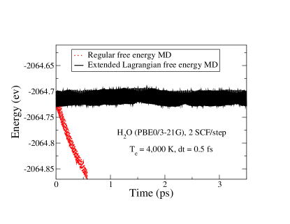
Figure 1: (Color online) The fluctuations in the total free energy, $E^{\rm tot}_{F}=E_{\rm K}+U-T_{e}{\cal S}$, of a water molecule using regular free energy molecular dynamics for a conventional density matrix based Born-Oppenheimer method with a linear extrapolation of the electronic state, Eq. (32), in comparison to the density matrix extended Lagrangian free energy molecular dynamics.

Figure 2 shows the free energy conservation vs. the fluctuations of the sum of the nuclear kinetic and potential energy, $E_{\rm K}+U$. Only one or two SCF cycles per time step are used, which shows that the simulation is stable, conserving the free energy under incomplete approximate SCF convergence. While the amplitude of the fluctuations in $E_{\rm K}+U$ is dependent on the electronic temperature $T_{e}$, the amplitude of the total free energy oscillations, $E^{\rm tot}_{F}=E_{\rm K}+U-T_{e}{\cal S}$, is not. This is an agreement with the total free energy being a constant of motion as in the density matrix extended free energy Lagrangian, Eq. (1), in the limit $\mu\rightarrow 0$.

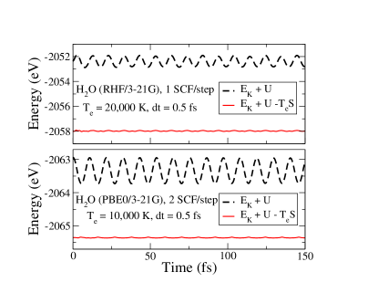
Figure 2: (Color online) The fluctuations in the nuclear kinetic and potential energy, $E_{\rm K}+U$, in comparison to the total free energy, $E^{\rm tot}_{F}=E_{\rm K}+U-T_{e}{\cal S}$, for a density matrix extended Lagrangian free energy molecular dynamics simulation of a single water molecule using Hartree-Fock (RHF) or hybrid density functional theory (PBE0 Adamo et al. (1999)). The average nuclear temperature was approximately room temperature, i.e. $T_{\rm ion}\approx 300$ K.

Figure 3 shows the corresponding behavior of the free energy fluctuations of the sum of the nuclear kinetic and potential energy, $E_{\rm K}+U$ for a single water molecule embedded in a C₆₀ Bucky ball. The electronic temperature was set to $T_{e}=5,000$ K, while the nuclear temperature of the Bucky ball was initially zero, and the water molecule was given an initial velocity and hence had a non-zero initial temperature. The time evolution of the total temperature, $T$, the temperature of only the Bucky ball, $T_{\mathrm{C60}}$, and the temperature of only the water molecule, $T_{\mathrm{water}}$, are shown in Figure 4. Clearly visible in the figure is the process of kinetic energy transfer from the water molecule to the Bucky ball; as the water molecule repeatedly collides with the wall of the Bucky ball, kinetic energy is transferred between the two sub-systems and the Bucky ball heats up, while the water molecule cools down.

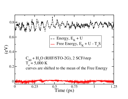
Figure 3: (Color online) The fluctuations in the nuclear kinetic and potential energy, $E_{\rm K}+U$, in comparison to the total free energy, $E^{\rm tot}_{F}=E_{\rm K}+U-T_{e}{\cal S}$, for a density matrix extended Lagrangian free energy molecular dynamics simulation of a single water molecule embedded within a $C_{60}$ Bucky ball using Hartree-Fock theory. The average nuclear temperature was approximately $T_{\rm ion}\approx 1000$ K.

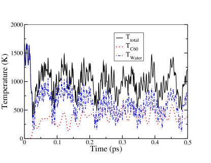
Figure 4: (Color online) The fluctuations in the total nuclear temperature, $T_{\mathrm{total}}$, in comparison with the temperature of only the Bucky ball, $T_{\mathrm{C60}}$ and the temperature of the water molecule, $T_{\mathrm{water}}$. We start our simulation with the Bucky ball at $T_{\mathrm{C60}}=0$ K and a water molecule at the center inside the Bucky ball with a non-zero initial velocity. While the total temperature remains fairly constant, the energy transfer from the water molecule to the Bucky ball is clearly visible in the rising $T_{\mathrm{C60}}$ and the falling $T_{\mathrm{water}}$.

If we use the original expression of the Pulay term Pulay (1969),

$${\cal F}^{\rm P}=2\mathrm{Tr}[{\widetilde{D}}{\widetilde{F}}{\widetilde{D}}(\partial S/\partial R_{k})],$$ (47)

which is valid only for an idempotent density matrix in the limit of $T_{e}=0$, i.e. when ${\widetilde{D}}={\widetilde{D}}S{\widetilde{D}}$, we find that it affects the energetics even at fairly modest electronic temperatures. Figure 5 gives a comparison of the free energy calculated either with the original zero-temperature expression in Eq. (47) or its finite temperature generalization in Eq. (29). Only the generalized Pulay force has the correct variational properties derived from the extended free energy Lagrangian, which gives a significant improvement in the conservation of the free energy.

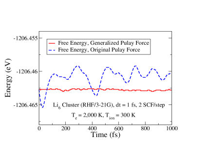
Figure 5: (Color online) The fluctuations in the total free energy, $E^{\rm tot}_{F}=E_{\rm K}+U-T_{e}{\cal S}$, for a small Li cluster at $T_{e}=2,000$ K simulated using FreeON within the density matrix extension. The Pulay force has been calculated either with the original zero-temperature expression, Eq. (47), or its finite temperature generalization, Eq. (29).

V.2.2 Plane wave extension

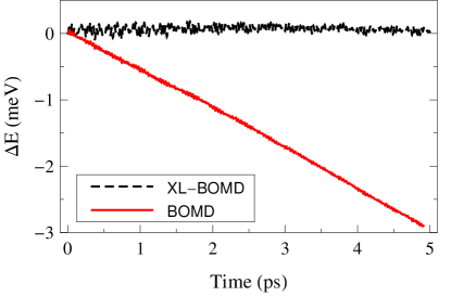
Figure 6: (Color online) The change in total free energy as a function of time for a periodic 8 atom silicon cell for conventional Born-Oppenheimer MD as implemented in VASP and extended Lagrangian free energy MD. Both simulations using a time step of 0.25 fs, and a energy convergence criteria of 0.5 meV. The conventional Born-Oppenheimer MD show a clear unphysical systematic drift in comparison to the extended Lagrangian free energy MD.

Figure 6 demonstrates how the total free energy for the conventional Born-Oppenheimer molecular dynamics and the plane wave extended Lagrangian free energy molecular dynamics behave over time in the plane wave formulation. A system of 8 silicon atoms are simulated for a total of 5 ps using a time step of 0.25 fs. The figure effectively depicts how the regular Born-Oppenheimer molecular dynamics exhibit an unphysical systematic drift in the total free energy. This issue is solved by the use of the extended Lagrangian free energy formulation, which with equivalent settings otherwise shows no systematic drift. In Fig. 7 we show the same behavior for the plane wave formulation as in Fig. 2 for the density formulation, where we demonstrate that the total free energy is a constant of motion. Figure 8 shows the error as measured by the amplitude of the total energy vs. the free energy fluctuations for various lengths of the integration time step $\delta t$. Only the free energy has the correct scaling with respect to the time step.

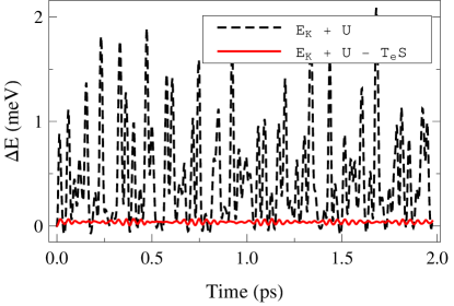
Figure 7: (Color online) The fluctuations for the total nuclear and potential energy, $E_{K}+U$, in comparison to the total free energy, $E_{K}+U+T_{e}S$, of a periodic 8 atom silicon system. The simulation was carried out using extend Lagrangian free energy MD in VASP. Using a time step of 0.25 fs and energy convergence criteria of $5\times 10^{-10}$ eV with ultrasoft pseudopotentials. Both the nuclear and electronic had an average temperature of about 500 K.

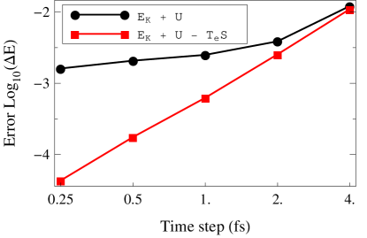
Figure 8: (Color online) The error amplitudes as a function of time step for the total nuclear and potential energy, $E_{K}+U$, and the total free energy, $E_{K}+U+T_{e}S$, of a 8 atom periodic silicon cell

V.3 Fermi operator expansion

The temperature-dependent density matrices for the simulations in Fig. 2 were constructed using the “exact” analytic Fermi-Dirac distribution of the states. If we instead use the recursive Fermi operator expansion of Algorithm 1 we find no significant deviation compared to the Fermi-Dirac result when we use more than 5 steps in the recursion. Figure 9 shows the free energy calculated with the exact result vs. the recursive expansion. The example corresponds to the simulation of the lower panel in Fig. 2. Using 5 recursion steps gives only a small constant shift in the free energy. The accuracy for a specific expansion order $m$ will depend on the temperature $T_{e}$. In Fig. 10 we show the error in the entropy as a function of $m$ for three different temperatures for a small Li cluster. In this case we find that the relative accuracy is reduced for lower temperatures, though the rate of convergence as a function of the number of expansion steps $m$ is the same.

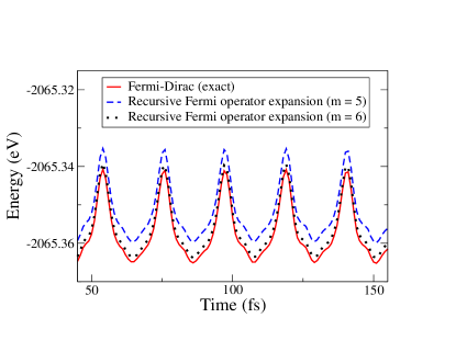
Figure 9: (Color online) The fluctuations in the total free energy, $E^{\rm tot}_{F}=E_{\rm K}+U-T_{e}{\cal S}$, for a water molecule, H₂O (PBE0/3-21G), using either the exact Fermi-Dirac distribution or the recursive Fermi operator expansion, Algorithm 1, with 5 ($m=5$) or 6 ($m=6$) recursion steps. The simulation is based on a hybrid density functional (PBE0 Adamo et al. (1999)) for $T_{e}=10,000$ K and $T_{\rm ion}\approx 300$ K using 2 SCF cycles per time step, $\delta t=0.5$ fs, within the density matrix extension.

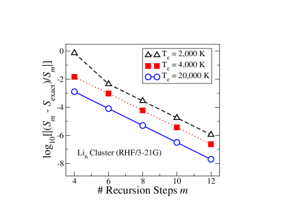
Figure 10: (Color online) The relative error in the entropy as a function of the number of expansion steps $m$ in the recursive Fermi operator expansion, Algorithm 1, for three different electronic temperatures $T_{e}$.

VI Summary and Discussion

Free energy generalizations of regular Born-Oppenheimer molecular dynamics for simulations at finite electronic temperatures are currently widely used Weinert and Davenport (1992); Wentzcovitch et al. (1992); Kresse and Furthmuller (1996); Marzari et al. (1997). In this paper first principles free energy molecular dynamics schemes were developed based on extended Lagrangian Born-Oppenheimer molecular dynamics Niklasson et al. (2006); Niklasson (2008a); Niklasson et al. (2009); Steneteg et al. (2010). The formulation was given both for density matrix and plane wave representations. The density matrix formulation has numerically convenient expressions for the electronic forces as well as a recursive Fermi operator expansion that are well suited for reduced complexity calculations. Our extended Lagrangian free energy molecular dynamics enables efficient and accurate molecular dynamics simulations based on Hartree-Fock and density functional theory (or any of their many extensions) both for localized orbital and plane wave pseudopotential calculations with a temperature-dependent electronic degrees of freedom and nuclear trajectories that evolve on the self-consistent free energy potential surface.

VII Acknowledgment

The Los Alamos National Laboratory is operated by Los Alamos National Security, LLC for the NNSA of the USDoE under Contract No. DE-AC52-06NA25396. We gratefully acknowledge the support of the US Department of Energy through the LANL LDRD/ER program and the Swedish Foundation for Strategic Research (SSF) via Strategic Materials Research Center on Materials Science for Nanoscale Surface Engineering (MS2E), and The Göran Gustafsson Foundation for Research in Natural Sciences and Medicine for this work. Discussions with Marc Cawkwell, Erik Holmström, Igor Abrikosov and Anders Odell as well as support from Travis Peery at the T-Division Ten-Bar Java Group are gratefully acknowledged.

Appendix A Recursive Fermi operator expansion

There are at least 19 different (dubious) ways to calculate matrix exponentials Moler and VanLoan (2003). Consider

$$e^{x}=\left(e^{x/n}\right)^{n}=\left(\frac{e^{x/(2n)}}{e^{-x/(2n)}}\right)^{n},$$ (48)

which after a first order Taylor expansion gives

$$e^{x}=\lim_{n\rightarrow\infty}\left(\frac{2n+x}{2n-x}\right)^{n}.$$ (49)

This means that the Fermi-Dirac distribution function, ${\Phi}(x)$, can be approximated as

$${\Phi}(x)=[e^{x}+1]^{-1}=\lim_{n\rightarrow\infty}\frac{(2n-x)^{n}}{(2n+x)^{n}+(2n-x)^{n}},$$ (50)

such that

$${\Phi}(2n-4nx)\approx\frac{x^{n}}{x^{n}+(1-x)^{n}}$$ (51)

for large values of $n$. The function

$${f}_{n}(x)=\frac{x^{n}}{x^{n}+(1-x)^{n}}$$ (52)

has the important recursive property,

$${f}_{m\times n}(x)={f}_{m}({f}_{n}(x)),$$ (53)

which enables a rapid high-order expansions. The following recursive approximation can therefore be used:

$${\Phi}\left[\beta(\varepsilon_{i}-\mu)\right] = {\Phi}(2n-4nx_{i})$$

$$\approx{f}_{n}(x_{i}) = {f}_{2}({f}_{2}(\ldots{f}_{2}(x_{i})\ldots)),$$ (54)

where

$$x_{i}=\frac{1}{2}-\frac{\beta}{4n}(\varepsilon_{i}-\mu)$$ (55)

and with the recursion repeated $m$ times, i. e. for $n=2^{m}$.

The density matrix at finite electronic temperatures,

$$D=\left[e^{\beta(H-\mu I)}+1\right]^{-1}={\Phi}\left[\beta(H-\mu I)\right],$$ (56)

can thus be calculated using the recursive grand canonical Fermi operator expansion,

$$D={f}_{2}\left(\ldots f_{2}\left({f}_{2}\left(\frac{1}{2}I-2^{-(2+m)}\beta(H-\mu I)\right)\right)\ldots\right),$$ (57)

which is generated by Algorithm 1.

Appendix B Constant energy integration: a practical guide

B.1 Underlying approximations

Even if a correct geometric and long-term energy conserving integration scheme, such as the Verlet algorithm, is used both for the nuclear and the electronic degrees of freedom, a systematic energy drift may still appear in a simulation. The most probable cause is the approximate formulation of the underlying dynamics. Any self-consistent first principles calculation involves many different numerical approximations, of which some can be physically motivated, others not. In the ideal case we would perform all calculations numerically exact, but for an approximate underlying dynamics that is sufficiently close to our effective single particle theory. The dominating major approximations due to incomplete SCF convergence and the finite time steps are treated within the extended Lagrangian framework and the geometric integration presented here. Other approximations, such as truncated multipole expansions, finite arithmetics, thresholding of small matrix elements, and finite grid errors, have not been considered. First principles electronic structure codes have in general never been able to generate exact energy conserving molecular dynamics. To obtain a well working scheme that is stable and energy conserving under approximate SCF convergence may thus involve extensive prior testing, tuning and debugging, even if the dissipative electronic force discussed above is applied. In this way, an energy conserving extended Lagrangian free energy (or Born-Oppenheimer) molecular dynamics simulation is an excellent test and signature of a well working code.

B.2 Thermostats

In regular Born-Oppenheimer molecular dynamics simulations, various forms of thermostats are applied to generate, for example, stable constant temperature (NVT) or constant pressure (NVP) ensembles. In this case the problem with a systematic energy drift may not be seen directly, but the underlying dynamics is, of course, still wrong, even if a hypothetical “exact” thermostat could be used. By using an ever increasing number of SCF cycles the underlying energy drift can be kept low, but this is computationally expensive. Thermostats typically act through a rescaling of the forces or the velocities of the nuclear degrees of freedom. Unfortunately, this approach may lead to an unphysical energy transfer between high-frequency and low-frequency modes Harvey et al. (1998). The problem is particularly significant when there is a large difference between the atomic masses Fukushi et al. (2000).

B.3 Practical guide

Depending on the accuracy of the electronic structure code used in the molecular dynamics simulation, we give the following practical guide for a constant free energy simulation: 1) Use the extended Lagrangian formulation Niklasson (2008a) and a geometric integration scheme Verlet (1967); Leimkuhler and Skeel (1994); Niklasson (2008a); Odell et al. (2009) for the integration of both the nuclear and the electronic degrees of freedom. 2) If the calculation is noisy, use electronic dissipation Niklasson et al. (2009), e.g. as in Eq. (35). 3) If the simulation still shows excessive fluctuations in the energy or a systematic drift we suggest a careful review and tuning of the numerical approximations in the underlying electronic description. 4) If the energetics still is unstable, and then only as a last resort, one could use a stabilizing velocity or force rescaling. In that case we suggest the following velocity rescaling, which is constructed to minimize the perturbation of the molecular trajectories:

$$c_{n}=\sqrt{1+\frac{\delta t}{\tau}\left(\frac{E_{F}^{0}-E_{F}^{\rm tot}(n)}{E_{\rm K}(n)}+\gamma\sum_{j=1}^{n-1}\frac{E_{F}^{0}-E_{F}^{\rm tot}(j)}{E_{\rm K}(j)}\right)},$$ (58)

$${\bf v}_{i}\rightarrow c_{n}{\bf v}_{i}.$$ (59)

Here ${\bf v}_{i}$ is the velocity of particle $i$, which is rescaled by the constant $c_{n}$ at time step $n$. $E_{F}^{0}$ is the desired target (free) energy, $E_{F}^{\rm tot}(n)=E_{\rm K}+U-T_{e}{\cal S}$ is the total (free) energy and $E_{\rm K}(n)$ is the nuclear kinetic energy at time step $n$. The constant $\tau$ is a chosen relaxation time and $\gamma$ is a weight factor for the integrated error term. The rescaling above is loosely based on the Berendsen thermostat Berendsen et al. (1984) including an integrated error term (if we chose $|\gamma|>0$) as is often used in conventional control theory. The velocity rescaling factor $c_{n}$ is typically small and if the Verlet integration scheme is used, $c_{n}$ scales with the length of the integration step $\delta t$ as $c_{n}=1+{\cal O}(\delta t^{3})$ or $c_{n}=1+{\cal O}(\delta t^{2})$, depending on how the relaxation time $\tau$ is chosen. For higher-order integration schemes, $c_{n}=1+{\cal O}(\delta t^{k})$ for larger integers of $k$. This means that even if the velocity rescaling is unphysical, the error can at least be kept very small, with only minor perturbations of the molecular trajectories. The velocity rescaling above was not necessary for any of the simulations performed for this article.

References

- Marx and Hutter (2000) D. Marx and J. Hutter, Modern Methods and Algorithms of Quantum Chemistry (ed. J. Grotendorst, John von Neumann Institute for Computing, Jülich, Germany, 2000), 2nd ed.
- Pulay and Fogarasi (2004) P. Pulay and G. Fogarasi, Chem. Phys. Lett. 386, 272 (2004).
- Niklasson et al. (2006) A. M. N. Niklasson, C. J. Tymczak, and M. Challacombe, Phys. Rev. Lett. 97, 123001 (2006).
- Niklasson (2008a) A. M. N. Niklasson, Phys. Rev. Lett. 100, 123004 (2008a).
- Roothaan (1951) C. C. J. Roothaan, Rev. Mod. Phys. 23, 69 (1951).
- Hohenberg and Kohn (1964) P. Hohenberg and W. Kohn, Phys. Rev. 136, B:864 (1964).
- Kohn and Sham (1965) W. Kohn and L. J. Sham, Phys. Rev. 140, 1133 (1965).
- Mermin (1965) N. D. Mermin, Phys. Rev. 137, A1441 (1965).
- Parr and Yang (1989) R. G. Parr and W. Yang, Density-functional theory of atoms and molecules (Oxford University Press, Oxford, 1989).
- Steneteg et al. (2010) P. Steneteg, I. A. Abrikosov, V. Weber, and A. M. N. Niklasson, Phys. Rev. B 82, 075110 (2010).
- Sanville et al. (2010) E. J. Sanville N. Bock, W. M. Challacombe, A. M. N. Niklasson, M. J. Cawkwell, T. D. Sewell, D. M. Dattelbaum, and S. Sheffield, Proceedings of the Fourteenth International Detonation Symposium, Office of Naval Research, Arlington VA, ONR-351-10-185, 91 (2010).
- Zheng et al. (2011) G. Zheng A. M. N. Niklasson and M. Karplus, J. Chem. Phys. 135, 044122 (2011).
- Niklasson and Weber (2007) A. M. N. Niklasson and V. Weber, J. Chem. Phys. 127, 064105 (2007).
- Weinert and Davenport (1992) M. Weinert and J. W. Davenport, Phys. Rev. B 45, R13709 (1992).
- Wentzcovitch et al. (1992) R. M. Wentzcovitch, J. L. Martins, and P. B. Allen, Phys. Rev. B 45, R11372 (1992).
- Car and Parrinello (1985) R. Car, and M. Parrinello, Phys. Rev. Lett. 55, 2471 (1985).
- Hartke and Carter (1992) B. Hartke, and E. A. Carter, Chem. Phys. Lett. 189, 358 (1992).
- Schlegel et al. (2001) H. B. Schlegel, J. M. Millam, S. S. Iyengar, G. A. Voth, A. D. Daniels, G. Scusseria, and M. J. Frisch, J. Chem. Phys. 114, 9758 (2001).
- Herbert and Head-Gordon (2004) J. Herbert and M. Head-Gordon, J. Chem. Phys. 121, 11 542 (2004).
- Pulay (1969) P. Pulay, Mol. Phys. 17, 197 (1969).
- Schlegel (2000) H. B. Schlegel, Theor. Chem. Acc. 103, 294 (2000).
- Niklasson (2008b) A. M. N. Niklasson, J. Chem. Phys. 129, 244107 (2008b).
- Jakowski and Morokuma (2009) J. Jakowski and K. Morokuma, J. Chem. Phys. 130, 224106 (2009).
- Warren and Dunlap (1996) R. W. Warren and B. I. Dunlap, Chem. Phys. Lett. 262, 384 (1996).
- Leimkuhler and Skeel (1994) B. J. Leimkuhler and R. D. Skeel, J. Comput. Phys. 112, 117 (1994).
- Odell et al. (2009) A. Odell, A. Delin, B. Johansson, N. Bock, M. Challacombe, and A. M. N. Niklasson (2009), j. Chem. Phys.
- Verlet (1967) L. Verlet, Phys. Rev. 159, 98 (1967).
- Payne et al. (1992) M. C. Payne, M. P. Teter, D. C. Allan, T. A. Arias, and J. D. Joannopoulos, Rev. Mod. Phys. 64, 1045 (1992).
- Arias et al. (1992) T. Arias, M. Payne, and J. Joannopoulos, Phys. Rev. Lett. 69, 1077 (1992).
- Millan et al. (1999) J. Millan, V. Bakken, W. Chen, L. Hase, and H. B. Schlegel, J. Chem. Phys. 111, 3800 (1999).
- Raynaud et al. (2004) C. Raynaud, L. Maron, J.-P. Daudey, and F. Jolibois, Phys. Chem. Phys. 6, 4226 (2004).
- Herbert and Head-Gordon (2005) J. Herbert and M. Head-Gordon, Phys. Chem. Chem. Phys. 7, 3269 (2005).
- Leimkuhler and Reich (2004) B. Leimkuhler and S. Reich (Cambridge University Press, 2004).
- Niklasson et al. (2009) A. M. N. Niklasson, P. Steneteg, A. Odell, N. Bock, M. Challacombe, C. J. Tymczak, E. Holmström, G. Zheng, and V. Weber (2009), j. Chem. Phys.
- Mead (1992) C. A. Mead, Rev. Mod. Phys. 64, 51 (1992).
- Niklasson (2003) A. M. N. Niklasson, Phys. Rev. B 68, 233104 (2003).
- Matsubara (1955) T. Matsubara, Prog. Theor. Phys. 14, 351 (1955).
- Mahan (1981) G. D. Mahan (Plenum, New York, 1981).
- Goedecker (1993) S. Goedecker, Phys. Rev. B 48, 17573 (1993).
- Bernstein (2001) N. Bernstein, Europhys. Lett 55, 52 (2001).
- Goedecker and Colombo (1994) S. Goedecker and L. Colombo, Phys. Rev. Let. 73, 122 (1994).
- Goedecker and Teter (1995) S. Goedecker and M. Teter, Phys. Rev. B 51, 9455 (1995).
- Silver et al. (1996) R. N. Silver, H. Roder, A. F. Voter, and J. D. Kress, Int. J. Comput. Phys. 124, 115 (1996).
- Goedecker (1999) S. Goedecker, Rev. Mod. Phys. 71, 1085 (1999).
- Liang et al. (2003) W. Z. Liang, C. Saravanan, Y. Shao, R. Baer, A. T. Bell, and M. Head-Gordon, J. Chem. Phys. 119, 4117 (2003).
- Ozaki (2007) T. Ozaki, Phys. Rev. B 75, 035123 (2007).
- Ceriotti et al. (2008) M. Ceriotti, T. D. Kühne, and M. Parrinello, J. Chem. Phys. 129, 024707 (2008).
- Golub and van Loan (1996) G. Golub and C. F. van Loan, Matrix Computations (Johns Hopkins University Press, Baltimore, 1996).
- Niklasson (2002) A. M. N. Niklasson, Phys. Rev. B 66, 155115 (2002).
- Niklasson et al. (2003) A. M. N. Niklasson, C. J. Tymczak, and M. Challacombe, J. Chem. Phys. 118, 8611 (2003).
- Rubensson and Salek (2005) E. H. Rubensson and P. Salek, J. Comput. Chem 26, 1628 (2005).
- Rubensson et al. (2008) E. H. Rubensson, E. Rudberg, and P. Salek, J. Chem. Phys. 128, 074106 (2008).
- Daw (1993) M. S. Daw, Phys. Rev. B 47, 10895 (1993).
- Li et al. (1993) X. P. Li, R. W. Nunes, and D. Vanderbilt, Phys. Rev. B 47, 10891 (1993).
- Palser and Manolopoulos (1998) A. H. R. Palser and D. E. Manolopoulos, Phys. Rev. B 58, 12704 (1998).
- Rubensson and Rudberg (2011) E. H. Rubensson and E. Rudberg, J. Phys.: Condes. Matter 23, 075502 (2011).
- Rubensson (2011) E. H. Rubensson, J. Chem. Theory Comput. 7, 1233 (2011).
- Adamo et al. (1999) C. Adamo, M. Cossi, and V. Barone, Theochem 493, 145 (1999).
- Bock et al. (2010) N. Bock, M. Challacombe, C. K. Gan, G. Henkelman, K. Nemeth, A. M. N. Niklasson, A. Odell, E. Schwegler, C. J. Tymczak, and V. Weber, FreeON (2010), Los Alamos National Laboratory (LA-CC 01-2; LA-CC-04-086), Copyright University of California., URL http://freeon.org/.
- Kresse and Furthmuller (1996) G. Kresse and J. Furthmuller, Phys. Rev. B 54, 11169 (1996).
- Vanderbilt (1990) D. Vanderbilt, Phys. Rev. B 41, 7892 (1990).
- Pulay (1980) P. Pulay, Chem. Phys. Let. 73, 393 (1980).
- Wood and Zunger (1985) D. Wood and A. Zunger, J. Phys. A. 18, 1343 (1985).
- Marzari et al. (1997) N. Marzari, D. Vanderbilt, and M. C. Payne, Phys. Rev. Lett. 79, 1337 (1997).
- Moler and VanLoan (2003) C. Moler and C. VanLoan, SIAM Review 45, 3 (2003).
- Harvey et al. (1998) S. Harvey, R. K.-Z. Tan, and T. E. C. III, J. Comput. Chem. 19, 726 (1998).
- Fukushi et al. (2000) D. Fukushi, K. Mae, and T. Honda, Jpn. J. Appl. Phys. 39, 5014 (2000).
- Berendsen et al. (1984) H. J. C. Berendsen, J. P. M. Postma, W. F. vanGundteren, A. DiNola, and J. R. Haak, J. Chem. Phys. 81, 3684 (1984).