Interquark potential for the charmonium system with almost physical quark masses

Abstract:

We study an interquark $\QQbar$ potential for the charmonium system, that is determined from the the equal-time and Coulomb gauge $\QQbar$ Bethe-Salpeter (BS) wavefunction through the effective Schrödinger equation. This novel approach enables us to evaluate a kinetic heavy quark mass $m_{Q}$ and a proper interquark potential at finite quark mass $m_{Q}$, which receives all orders of $1/m_{Q}$ corrections on the static $\QQbar$ potential from Wilson loops, simultaneously. Precise information of the interquark potential for both charmonium and bottomonium states directly from lattice QCD provides us a chance to improve quark potential models, where the spin-independent interquark potential is phenomenologically described by the Cornell potential and the spin-dependent parts are deduced within the framework of perturbative QCD, from first-principles calculations. In this study, calculations are carried out in both quenched and dynamical fermion simulations. We first demonstrate that the interquark potential at finite quark mass calculated by the BS amplitude method smoothly approaches the conventional static heavy quark potential from Wilson loops in the infinitely heavy quark limit within quenched lattice QCD simulations. Secondly, we determine both spin-independent and -dependent parts of the interquark potential for the charmonium system in 2+1 flavor dynamical lattice QCD using the PACS-CS gauge configurations at the lightest pion mass, $M_{\pi}=156$ MeV.

1 Introduction

The linearly rising interquark potential in QCD plays an essential role in the formation of hadrons. Indeed, the quarkonium states such as charmonia and bottomonia can be described well by quark potential models [1, 2, 3], where the Coulomb plus linear potential, the so-called Cornell potential, is phenomenologically adopted as the spin-independent central potential. One of the major successes of lattice QCD is to demonstrate that the static Wilson loop gives a confining potential between infinitely heavy quark ($Q$) and antiquark ($\overline{Q}$), which support the phenomenology of confining quark interactions in the heavy $Q\overline{Q}$ system [4].

As for the spin-dependent potential, spin-spin, tensor and spin-orbit terms of the interquark potential can be identified as relativistic corrections to the static $Q\overline{Q}$ potential, which are classified in powers of $1/m_{Q}$ within a framework called potential non-relativistic QCD (pNRQCD) [5]. However, although the spin-spin potential have been precisely calculated as one of the next-leading order corrections in quenched lattice QCD [6], their attractive spin-spin potential does not even qualitatively agree with the corresponding one in quark potential models, where the repulsive spin-spin interaction is phenomenologically required by heavy quarkonium spectroscopy. The spin-spin interaction calculated within the Wilson loop formalism seems to yield wrong mass ordering among hyperfine multiplets [6]. In potential models, functional forms of the spin-dependent terms are basically determined by perturbative one-gluon exchange [2]. Such the Fermi-Breit type potential, which appears at the order of $1/m_{Q}^{2}$ within pNRQCD, would have validity only at short distances and also in the vicinity of $m_{Q}=\infty$. The $1/m_{Q}$ expansion is not formally applicable at the charm quark mass. Therefore, properties of higher-mass charmonium states predicated in potential models may suffer from large uncertainties in this sense.

Under these circumstances, we have succeeded to determine a proper interquark potential at finite quark mass from the equal-time and Coulomb gauge Bethe-Salpeter (BS) amplitude through an effective Schrödinger equation [7, 8]. (See also Ref. [9]). In this proceedings, we will discuss the quark mass dependence of the spin-independent interquark potential in quenched lattice QCD [7] and then show results of both spin-independent and -dependent parts of the charmonium potential in 2+1 flavor full QCD with almost physical quark masses [8].

2 Formulation

Let us briefly review the new method utilized here to calculate the interquark potential with the finite quark mass. As the first step, we consider the following equal-time $\QQbar$ BS wavefunction in the Coulomb gauge for the quarkonium states.

$$\phi_{\Gamma}({\bf r})=\sum_{{\bf x}}\langle 0|\overline{Q}({\bf x})\Gamma Q({\bf x}+{\bf r})|\QQbar;J^{PC}\rangle,$$ (1)

where ${\bf r}$ is the relative coordinate of two quarks and $\Gamma$ is any of the 16 Dirac $\gamma$ matrices. Practically, the BS wavefunction can be extracted from the following four-point correlation function

$$\sum_{{\bf x},{\bf x}^{\prime},{\bf y}^{\prime}}\langle 0|\overline{Q}({\bf x},t)\Gamma Q({\bf x}+{\bf r},t)\left(\overline{Q}({\bf x}^{\prime},t_{\rm s})\Gamma Q({\bf y}^{\prime},t_{\rm s})\right)^{\dagger}|0\rangle$$

$$=\sum_{{\bf x}}\sum_{n}A_{n}\langle 0|\overline{Q}({\bf x})\Gamma Q({\bf x}+{\bf r})|n\rangle e^{-M^{\Gamma}_{n}(t-t_{\rm s})}\ \ \ \xrightarrow{t\gg t_{\rm s}}\ \ \ A_{0}\phi_{\Gamma}({\bf r})e^{-M^{\Gamma}_{0}(t-t_{\rm s})},$$ (2)

at the large Euclidean time from source location ($t_{\rm s}$). Here both quark and anti-quark fields at $t_{\rm s}$ are separately averaged in space as wall sources. $M^{\Gamma}_{n}$ denotes a mass of the $n$-th quarkonium state $|n\rangle$ in a given $J^{PC}$ channel. For instance, $\Gamma$ is chosen to be $\gamma_{5}$ and $\gamma_{i}$ to obtain the rest mass of the pseudo-scalar (PS) state $(J^{PC}=0^{-+})$ and vector (V) state $(J^{PC}=0^{--})$, respectively.

The BS wavefunction satisfies the Schrödingier equation with a non-local potential $U$ [10]

$$-\frac{\nabla^{2}}{m_{Q}}\phi_{\Gamma}({\bf r})+\int d{\bf r}^{\prime}U({\bf r},{\bf r}^{\prime})\phi_{\Gamma}({\bf r}^{\prime})=E_{\Gamma}\phi_{\Gamma}({\bf r}),$$ (3)

where $m_{Q}$ denotes the quark kinetic mass. The energy eigenvalue $E_{\Gamma}$ of the stationary Schrödinger equation is supposed to be $M_{\Gamma}-2m_{Q}$. If the relative quark velocity $v=|{\nabla}/m_{Q}|$ is small as $v\ll 1$, the non-local potential $U$ can generally expand in terms of the velocity $v$ as $U({\bf r}^{\prime},{\bf r})=\{V(r)+V_{\text{S}}(r){\mathbf{S}}_{Q}\cdot{\mathbf{S}}_{\overline{Q}}+V_{\text{T}}(r)S_{12}+V_{\text{LS}}(r){\bf L}\cdot{\bf S}+\mathcal{O}(v^{2})\}\delta({\bf r}^{\prime}-{\bf r})$, where $S_{12}=({\mathbf{S}}_{Q}\cdot\hat{r})({\mathbf{S}}_{\overline{Q}}\cdot\hat{r})-{\mathbf{S}}_{Q}\cdot{\mathbf{S}}_{\overline{Q}}/3$ with $\hat{r}={\bf r}/r$, ${\bf S}={\mathbf{S}}_{Q}+{\mathbf{S}}_{\overline{Q}}$ and ${\bf L}={\bf r}\times(-i\nabla)$ [10]. Here, $V$, $V_{\text{S}}$, $V_{\text{T}}$ and $V_{\text{LS}}$ represent the spin-independent central, spin-spin, tensor and spin-orbit potentials, respectively.

In this study, we focus only on the $S$-wave states. Thus we perform an appropriate projection with respect to the discrete rotation, which provides the BS wavefunction projected in the $A^{+}_{1}$ representation. The Schrödinger equation for the projected BS wavefunction $\phi_{\Gamma}(r)$ is reduced to

$$\left\{-\frac{\nabla^{2}}{m_{Q}}+V(r)+{\mathbf{S}}_{Q}\cdot{\mathbf{S}}_{\overline{Q}}V_{\text{S}}(r)\right\}\phi_{\Gamma}(r)=E_{\Gamma}\phi_{\Gamma}(r)$$ (4)

at the leading order of the $v$-expansion. The spin operator ${\mathbf{S}}_{Q}\cdot{\mathbf{S}}_{\overline{Q}}$ can be easily replaced by expectation values. As a result, both spin-independent and -dependent interquark potentials can be separately evaluated through a linear combination of Eq.(4) calculated for PS and V channels as

$$V(r) = E_{\text{ave}}+\frac{1}{m_{Q}}\left\{\frac{3}{4}\frac{\nabla^{2}\phi_{\text{V}}(r)}{\phi_{\text{V}}(r)}+\frac{1}{4}\frac{\nabla^{2}\phi_{\text{PS}}(r)}{\phi_{\text{PS}}(r)}\right\}$$ (5)

$$V_{\text{S}}(r) = E_{\text{hyp}}+\frac{1}{m_{Q}}\left\{\frac{\nabla^{2}\phi_{\text{V}}(r)}{\phi_{\text{V}}(r)}-\frac{\nabla^{2}\phi_{\text{PS}}(r)}{\phi_{\text{PS}}(r)}\right\},$$ (6)

where $E_{\text{ave}}=M_{\text{ave}}-2m_{Q}$ and $E_{\text{hyp}}=M_{\text{V}}-M_{\text{PS}}$. The mass $M_{\text{ave}}$ denotes the spin-averaged mass as $\frac{1}{4}M_{\text{PS}}+\frac{3}{4}M_{\text{V}}$. The derivative $\nabla^{2}$ is defined by the discrete Laplacian with nearest-neighbor points.

Note here that quark kinetic mass $m_{Q}$ is essentially required in the definition of the interquark potentials. Under a simple, but reasonable assumption as $\lim_{r\to\infty}V_{S}(r)=0$, which implies that there is no long-range correlation and no irrelevant constant term in the spin-dependent potential, we can obtain the quark kinetic mass from the following formula,

$$m_{Q}=\lim_{r\to\infty}\frac{-1}{E_{\text{hyp}}}\left\{\frac{\nabla^{2}\phi_{\text{V}}(r)}{\phi_{\text{V}}(r)}-\frac{\nabla^{2}\phi_{\text{PS}}(r)}{\phi_{\text{PS}}(r)}\right\}.$$ (7)

3 Numerical results

We have performed lattice QCD simulations in both quenched and full QCD in this study.

3.1 $N_{f}=0$ quenched QCD simulation

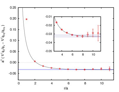
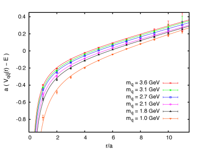
Figure 1: (left) A typical result of $\nabla^{2}\phi_{\rm V}/\phi_{\rm V}-\nabla^{2}\phi_{\rm PS}/\phi_{\rm PS}$ as a function of spacial distance $r$. (right) The interquark potential calculated from the $\QQbar$ BS amplitude at finite quark masses covering the range from 1.0 to 3.6 GeV. Each curve represents the fit result with the Cornell parametrization.

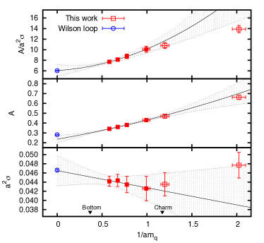
Figure 2: The quark-mass dependence of $A/\sigma$, $A$, and $\sigma$ as functions of $1/m_{Q}$. We perform the extrapolation towards the $m_{Q}\rightarrow\infty$ limit (solid curves) of $A/\sigma$, $A$, and $\sigma$ with a simple polynomial function in $1/m_{Q}$. For $\sigma$, a linear fit with respect to $1/m_{Q}$ is enough to describe the data with reasonable $\chi^{2}/{\rm d.o.f}$, while quadratic fits are used for $A/\sigma$ and $A$. The results given by Wilson loops are also included as open circles. .

In quenched lattice QCD simulations, we use a lattice size of $L^{3}\times T=32^{3}\times 48$ with the single plaquette gauge action at $\beta=6/g^{2}=6.0$, which corresponds to a lattice cutoff of $a^{-1}\approx 2.1$ GeV. The spatial lattice size corresponds to $La\approx 3\;{\rm fm}$. We fix the lattice to Coulomb gauge. The heavy-quark propagators are computed using the relativistic heavy-quark (RHQ) action with relevant one-loop coefficients of the RHQ [11, 12], which can remove large discretization errors introduced by large quark mass. To examine the infinitely heavy-quark limit, we adopt the six values of the hopping parameter $\kappa$, which cover the range of the spin-averaged mass of $1S$ quarkonium states $M_{\rm ave}=\frac{1}{4}(M_{\rm PS}+3M_{\rm V})=1.97$-5.86 GeV. We calculate quark propagators with a wall source located at $t_{\rm s}/a=4$. Our results are analyzed on 150 configurations for every hopping parameters.

First, in Fig. 1, we plot a difference of ratios of $\nabla^{2}\phi_{\rm V}/\phi_{\rm V}$ and $\nabla^{2}\phi_{\rm PS}/\phi_{\rm PS}$ as a function of spatial distance $r$ at $\kappa=0.10190$, which is close to the charm quark mass, as a typical example. The ratios of $\nabla^{2}\phi_{\Gamma}/\phi_{\Gamma}$ are evaluated by a weighted average of data points in the range of $(t-t_{\rm src})/a=$ 21 - 23. At a glance, the value of $\nabla^{2}\phi_{\rm V}/\phi_{\rm V}-\nabla^{2}\phi_{\rm PS}/\phi_{\rm PS}$ certainly reaches a nonzero constant value at large distances, which turns out to be the value of $-m_{Q}\Delta E_{\rm hyp}$. We then obtain the quark kinetic masses from the long-distance asymptotic values of $\nabla^{2}\phi_{\rm V}/\phi_{\rm V}-\nabla^{2}\phi_{\rm PS}/\phi_{\rm PS}$ divided by the measured hyperfine splitting $\Delta E_{\rm hyp}$.

Using the quark kinetic mass determined here, we can properly calculate the spin-independent interquark potential from the BS wavefunctions. Figure 1 displays results of our potential obtained at several quark masses. For clarity of the figure, the constant energy shift $E_{\text{ave}}$ is not subtracted. The resulting $\QQbar$ potentials at finite quark masses exhibit the linearly rising potential at large distances and the Coulomb-like potential at short distances as originally reported in Ref [9].

We simply adopt the Cornell parametrization for fitting our data $V(r)=-A/r+\sigma r+V_{0}$ with the Coulombic coefficient $A$, the string tension $\sigma$, and a constant $V_{0}$. All fits are performed over the range $1\leq r/a\leq 11$. In Fig. 2, we show the quark-mass dependence of $A/\sigma$, $A$ and $\sigma$ as functions of $1/m_{Q}$. First, regardless of the definition of $m_{Q}$, the ratio of $A/\sigma$ in the top figure indicates that the $\QQbar$ potential calculated from the BS wavefunction smoothly approaches the potential obtained from Wilson loops in the infinitely heavy-quark limit. If we pay attention to the quark-mass dependence of each of the Cornell parameters separately, we observe that, although the Coulombic parameter $A$ depends on the quark mass significantly, there is no appreciable dependence of the quark mass on the string tension $\sigma$. Their extrapolated values at $m_{Q}\rightarrow\infty$ are again consistent with those of the Wilson loop result. The extrapolation curve are also displayed as a solid curve in Fig. 2.

3.2 $N_{f}=2+1$ full QCD simulation

Table 1: Summary of RHQ parameters calibrated for charmonium system in dynamical QCD simulation.

	$\kappa_{c}$	$\nu$	$r_{s}$	$c_{B}$	$c_{E}$
RHQ parameters	0.10819	1.2153	1.2131	2.0268	1.7911

Full QCD simulations are also carried out by using 2+1 flavor gauge configurations generated by PACS-CS Collaboration on lattice of size $32^{3}\times 64$ with the Iwasaki gauge action at $\beta=1.9$, which corresponds to a comparable lattice cutoff of $a^{-1}\approx 2.2$ GeV  [13]. The spatial lattice size corresponds to $L\approx 3\;{\rm fm}$. The hopping parameters for the light sea quarks {$\kappa_{ud}$,$\kappa_{s}$}={0.13781, 0.13640} correspond to $M_{\pi}=156(7)$ MeV and $M_{K}=554(2)$ MeV [13]. Our results are analyzed on all 198 gauge configurations. We also employ RHQ action to compute the heavy quark propagator, which has five parameters $\kappa_{c}$, $\nu$, $r_{s}$, $c_{B}$ and $c_{E}$. The parameters $r_{s}$, $c_{B}$ and $c_{E}$ are determined by tadpole improved one-loop perturbation theory [12]. For $\nu$, we use a non-perturbatively determined value, which is adjusted as $c^{2}_{\text{eff}}=1$ in the dispersion relation $E^{2}({\bf p}^{2})=M^{2}+c^{2}_{\text{eff}}|{\bf p}|^{2}$ for the spin-averaged $1S$ charmonium state. We choose $\kappa_{c}$ to reproduce the experimental spin-averaged mass of $1S$ charmonium states $M_{\text{ave}}^{\text{exp}}=3.0678(3)$ GeV. As a result, the relevant speed of light, $c^{2}_{\text{eff}}=1.04(5)$, and the spin-averaged $1S$ charmonium mass, $M_{\text{ave}}=3.0702(9)$ GeV, is observed with our RHQ parameters summarized in Table 1. To increase statistics for BS wavefunction, we have computed charm quark propagators with two wall sources located at different time slices $t_{\rm s}/a=6$ and 57 and fold them together to create a single four-point correlation function. Then the measured hyperfine mass splitting $M_{\text{hyp}}=0.1137(8)$ GeV is close to the experimental value $M_{\text{hyp}}^{\text{exp}}=0.1166(12)$ GeV.

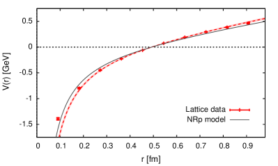
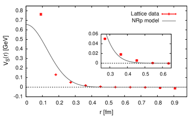
Figure 3: Spin-independent (left) and spin-dependent (right) parts of the central charmonium potential. The solid curves show the phenomenological potentials adopted in a NRp model [3]. The dashed curve appeared in the left panel represent a fit result with the Cornell parameterization.

First, we show a result of the spin-independent charmonium potential $V(r)$ with the fitted curve (dashed curve) in Fig. 3, where the constant term is subtracted to set $V(r_{0})=0$ with the Sommer scale, $r_{0}\approx 0.5$ fm. The Cornell parametrization is also simply adopted for fit. We have carried out correlated $\chi^{2}$ fits with full covariance matrix for on-axis data over range $4\leq r/a\leq 10$. The fitting results are listed in Table 2. The quoted errors represent only the statistical errors given by the jack-knife analysis. The phenomenological potential used in NRp models [3] is also plotted as a solid curve for comparison in Fig. 3. Although the charmonium potential obtained from lattice QCD is quite similar to the one in the NRp models, the string tension of the charmonium potential is slightly stronger than the phenomenological one. Therefore our result indicates that there are only minor modifications required for the spin-independent central potential in the NRp models. Moreover, it seems that a large gap for the Coulombic coefficients between the conventional static potential and the phenomenological potential is filled by our new approach, where all orders of $1/m_{Q}$ corrections are nonperturbatively accounted for.

Table 2: Summary of the Cornell parameters and the quark mass determined from lattice QCD. For comparison, the corresponding values adopted in a non-relativistic potential (NRp) model [3] are also included.

	This work	Polyakov lines	NRp model
$A$	0.861(17)	0.403(24)	0.7281
$\sqrt{\sigma}$ [GeV]	0.394(7)	0.462(4)	0.3775
$m_{Q}$ [GeV]	1.74(3)	$\infty$	1.4794

In Fig. 3, we next show the spin-spin term of the charmonium potential and the corresponding phenomenological one found in Ref. [3]. Our spin-spin potential exhibits the short range repulsive interaction, which is required by the charmonium spectroscopy. It should be reminded that the Wilson loop approach fails to reproduce the correct behavior of the spin-spin interaction, since the leading-order spin-spin potential classified in pNRQCD becomes attractive at short distances [6]. In contrast of the case of the spin-independent potential, the spin-spin potential obtained here is absolutely different from a repulsive $\delta$-function potential generated by perturbative one-gluon exchange. Indeed, the finite-range spin-spin potential described by the Gaussian form is adopted in Ref. [3], where many properties of conventional charmonium states at higher masses are predicted. This phenomenological spin-spin potential is also plotted in Fig. 3 for comparison. There still remains a slight difference between the spin-spin potential from first principles QCD and the phenomenological one. In this sense, the reliable spin-dependent potential derived from lattice QCD can provide new and valuable information to the NRp models.

4 Summary

We have proposed the new method to determine the interquark potential at finite quark mass from lattice QCD. Using quenched lattice QCD, we have demonstrated that the spin-independent central potential defined in this method smoothly approaches the static $\QQbar$ potential given by Wilson loops in the infinitely heavy-quark limit. In dynamical lattice QCD simulations, we have studied both spin-independent and -dependent parts of the charmonium potential. The spin-independent charmonium potential obtained from lattice QCD with almost physical quark masses is quite similar to the one used in the NRp models. The spin-spin potential properly exhibits the short range repulsive interaction. Its $r$-dependence, however, is slightly different from the phenomenological one adopted in Ref. [3]. Therefore, our charmonium potential derived from first principles QCD suggest that properties of higher-mass charmonium states predicted in the NRp models may change.

We acknowledge the PACS-CS collaboration and ILDG/JLDG for providing us with the gauge configurations. We would also like to thank H. Iida, Y. Ikeda and T. Hatsuda for fruitful discussions. This work was partially supported by JSPS/MEXT Grants-in-Aid (No. 22-7653, No. 19540265, No. 21105504 and No. 23540284).

References

- [1] E. Eichten et.al., Phys. Rev. Lett. 36, 500 (1976).
- [2] S. Godfrey and N. Isgur, Phys. Rev. D 32, 189 (1985).
- [3] T. Barnes, S. Godfrey and E. S. Swanson, Phys. Rev. D 72, 054026 (2005).
- [4] For a review, see G. S. Bali, Phys. Rept. 343, 1 (2001).
- [5] N. Brambilla et al., Rev. Mod. Phys. 77, 1423 (2005).
- [6] Y. Koma and M. Koma, Nucl. Phys. B 769, 79 (2007).
- [7] T. Kawanai and S. Sasaki, Phys. Rev. Lett. 107, 091601 (2011).
- [8] T. Kawanai and S. Sasaki, arXiv:1110.0888 [hep-lat].
- [9] Y. Ikeda and H. Iida, arXiv:1102.2097 [hep-lat].
- [10] N. Ishii, S. Aoki and T. Hatsuda, Phys. Rev. Lett. 99, 022001 (2007), S. Aoki, T. Hatsuda and N. Ishii, Prog. Theor. Phys. 123 (2010) 89.
- [11] S. Aoki, Y. Kuramashi and S. I. Tominaga, Prog. Theor. Phys. 109, 383 (2003).
- [12] Y. Kayaba et al. [CP-PACS Collaboration], JHEP 0702, 019 (2007).
- [13] S. Aoki et al. [PACS-CS Collaboration], Phys. Rev. D 79, 034503 (2009).