Excited state contamination in nucleon structure calculations

Abstract:

Among the sources of systematic error in nucleon structure calculations is contamination from unwanted excited states. In order to measure this systematic error, we vary the operator insertion time and source-sink separation independently. We compute observables for three source-sink separations between 0.93 fm and 1.39 fm using clover-improved Wilson fermions and pion masses as low as 150 MeV. We explore the use of a two-state model fit to subtract off the contribution from excited states.

1 Introduction

As Lattice QCD calculations of nucleon structure have been performed with decreasing pion mass, chiral extrapolations have become less able to reconcile lattice data with experiment [1, 2]. An important source of systematic error is contamination from excited states [3, 4], i.e. the failure to isolate the ground-state nucleon.

In order to compute nucleon matrix elements and form-factors, we compute nucleon two-point functions $C_{\text{2pt}}(T,\vec{p}^{\prime})$ and three-point functions $C_{\text{3pt}}^{\mathcal{O}}(T,\tau,\vec{p},\vec{p}^{\prime})$ on the lattice [5], where $T$ is the Euclidean time separation between the source and the sink, $\tau$ is the Euclidean time separation between the source and the operator $\mathcal{O}$, $\vec{p}^{\prime}$ is the sink momentum, and $\vec{p}$ is the source momentum. If the nucleon interpolating operator with momentum $\vec{p}$ creates $N$ states with energies $E_{n}(\vec{p})$, then the two-point and three-point functions have the form

$$\begin{split}C_{\text{2pt}}(T,\vec{p})&=\sum_{n=0}^{N-1}a_{n}(\vec{p})e^{-E_{n}(\vec{p})T}\\ C_{\text{3pt}}^{\mathcal{O}}(T,\tau,\vec{p},\vec{p}^{\prime})&=\sum_{n,n^{\prime}=0}^{N-1}\sqrt{a_{n}(\vec{p})a_{n^{\prime}}(\vec{p}^{\prime})}\sum_{i}M_{i}^{\mathcal{O}}F_{i}^{n\to n^{\prime}}(t)e^{-E_{n}(\vec{p})\tau-E_{n^{\prime}}(\vec{p}^{\prime})(T-\tau)},\end{split}$$ (1)

where $t=-(p^{\prime}-p)^{2}$, $F_{i}^{n\to n^{\prime}}(t)$ are transition form-factors for the transition from state $n$ to state $n^{\prime}$ via the operator $\mathcal{O}$, and $M$ is determined by kinematics and by the definition of the form-factors.

2 Computing form-factors

The traditional approach for computing nucleon matrix elements and form-factors is to use a ratio of three-point and two-point functions:

$$R^{\mathcal{O}}(T,\tau,\vec{p},\vec{p}^{\prime})=\frac{C_{\text{3pt}}^{\mathcal{O}}(T,\tau,\vec{p},\vec{p}^{\prime})}{\sqrt{C_{\text{2pt}}(T,\vec{p})C_{\text{2pt}}(T,\vec{p}^{\prime})}}\sqrt{\frac{C_{\text{2pt}}(T-\tau,\vec{p})C_{\text{2pt}}(\tau,\vec{p}^{\prime})}{C_{\text{2pt}}(T-\tau,\vec{p}^{\prime})C_{\text{2pt}}(\tau,\vec{p})}},$$

such that in the limit of large $\tau$ and $T-\tau$, where excited states have negligible contribution, the amplitudes $a_{0}(\vec{p})$, $a_{0}(\vec{p}^{\prime})$ and the exponential dependences on $\tau$ and $T-\tau$ are canceled. In practice, we compute these ratios for one or more fixed values of $T$ and $\tau\in[0,T]$, then for each $(T,\tau)$ we compute the form-factors $F_{i}(t)$ from an overdetermined fit to the ratios $R$. Then we produce “plateau plots” of $F_{i}(t)$ versus $\tau$, for fixed $T$, and look for a flat region where it is hoped that excited-state contamination is small.

The new approach introduced here is to do a combined fit to $C_{\text{2pt}}$ and $C_{\text{3pt}}$ using an $N$-state model derived from Eq. 1, for a small value of $N$. In order to further simplify the fit, we assume the dispersion relation $E_{n}^{2}(\vec{p})=m_{n}^{2}+\vec{p}^{2}$, and define

$$\tilde{F}_{i}^{n\to n^{\prime}}(t)=\sqrt{a_{n}(\vec{p})a_{n^{\prime}}(\vec{p}^{\prime})}F_{i}^{n\to n^{\prime}}(t),$$

so that for fixed masses, the fit model for $C_{\text{2pt}}$ and $C_{\text{3pt}}$ depends linearly on the fit parameters $a_{n}(\vec{p})$ and $\tilde{F}_{i}^{n\to n^{\prime}}(t)$. This enables the use of an iterative fitting procedure for the masses, where at each step the larger set of linear fit parameters is solved for exactly. Denoting the two-point and three-point functions to which we are fitting by $C_{\alpha}$ and the linear fit parameters by $b_{i}$, we minimize

$$\chi^{2}=(A_{\alpha i}(\{m_{n}\})b_{i}-C_{\alpha})(S^{*})_{\alpha\beta}^{-1}(A_{\beta j}(\{m_{n}\})b_{j}-C_{\beta}),$$

where $S^{*}_{\alpha\beta}$ is our estimate of the covariance matrix of $\{C_{\alpha}\}$. Because typically the number of independent samples that we have is of the same order as the number of variables $C_{\alpha}$, we use a shrinkage estimator of the covariance matrix [6], $S^{*}=(1-\lambda)S+\lambda T$, where $S$ is the sample covariance matrix, $T$ is its diagonal part, and $\lambda$ is estimated from the data such that the expected error of the correlation matrix $R_{\alpha\beta}\equiv S^{*}_{\alpha\beta}/\sqrt{S^{*}_{\alpha\alpha}S^{*}_{\beta\beta}}$ is asymptotically minimized [7].

If the number of states included in the model is less than the number of states that have non-negligible contributions to $C_{\text{2pt}}$ and $C_{\text{3pt}}$, then each model state will have to account for the contributions from more than one state in the lattice data. The best-fit masses in the model will be weighted averages of the masses of states that contribute to the data. The relevant weights are different for different correlators [8], so when doing a 2-state fit, we use a single ground-state mass $m_{0}$ but allow the excited-state mass in the model to vary, using one mass $m_{1}^{(2)}$ for $C_{\text{2pt}}$ and a different mass $m_{1}^{(3)}$ for $C_{\text{3pt}}$. The difference between these two masses is an indicator of the importance of omitted states.

3 Lattice measurements

We use 2+1 flavors of tree-level clover-improved Wilson fermions coupled to double-HEX-smeared gauge links [9]. Results presented here are from ensembles with lattice spacing $a=0.116$ fm and pion masses approximately 150, 200, and 250 MeV. At the lightest pion mass, the lattice volume is $48^{4}$, and at the other two it is $32^{3}\times 48$. In order to study excited-state contamination, we compute nucleon three-point functions with three different source-sink separations $T/a=8$, 10, and 12. We focus on isovector quantities to avoid contributions from disconnected diagrams. We use the standard nucleon operator, $N_{\alpha}=\epsilon^{abc}(u^{T}_{a}C\gamma_{5}d_{b})u_{c\alpha}$, where the quark fields have smearing tuned to minimize excited states seen in the two-point function, and we use the spin-parity projection $\Gamma_{\text{pol}}=\tfrac{1+\gamma_{4}}{2}\tfrac{1-i\gamma_{3}\gamma_{5}}{2}$. All of the errors below are statistical and are computed using the jackknife method.

Matrix elements of the vector current $V^{\mu}_{q}=\bar{q}\gamma^{\mu}q$ are parametrized by the vector form-factors $F_{1,2}(t)$. The mean squared Dirac radius is defined from the slope of $F_{1}(t)$ at zero $t$: $F_{1}(t)=F_{1}(0)[1-\tfrac{1}{6}(r_{1})^{2}t+\mathcal{O}(t^{2})]$. We compute the isovector Dirac radius from a linear fit to $F_{1}(0)$ and $F_{1}(t_{1})$, where $t_{1}$ corresponds to three-point functions with $\vec{p}$ equivalent to $\tfrac{2\pi}{L}(1,0,0)$, and $\vec{p}^{\prime}=0$. Using the ratio method, we average the three central points of each plateau plot to arrive at a value of $(r_{1}^{u-d})^{2}$ for each source-sink separation and each ensemble. The results are shown in Fig. 2. There is a consistent trend across the three ensembles of the Dirac radius increasing between $T/a=8$ and $T/a=10$. However, the behavior going to $T/a=12$ is ambiguous and it is unclear, from this analysis and with currently available statistics, whether or not excited-state contamination is still a problem at $T/a=10$.

We also compute the isovector average momentum fraction $\langle x\rangle^{u-d}$ from forward matrix elements of the operator $\mathcal{O}_{q}^{\mu\nu}=\bar{q}\gamma^{\{\mu}iD^{\nu\}}q$, where the braces denote taking the symmetric traceless part of the tensor. Note that the results presented here have not been renormalized. Again averaging the three central points of each plateau plot, the results are seen in Fig. 2. In this case, a clearer trend is visible: $\langle x\rangle^{u-d}$ decreases as $T/a$ increases, and there is no evidence that even $T/a=12$ might be large enough that excited-state contamination is negligible. This result is consistent with a recent study using the open sink method, where $\tau$ is fixed in order to allow the calculation of three-point functions at all values of $T$ [10]. Furthermore, the effect of excited states appears to be larger at smaller pion masses. This is consistent with the fact that earlier calculations at larger pion masses using domain wall valence fermions on an asqtad sea yielded chiral extrapolations to the physical point in excellent agreement with experiment [11, 12].

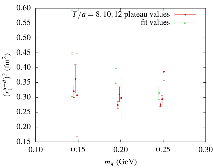
Figure 1: Isovector Dirac radius $(r_{1}^{u-d})^{2}$ ($\text{fm}^{2}$) versus $m_{\pi}$ (GeV). At each pion mass, from left to right are results obtained from the fitting procedure, and from the ratio method with three increasing source-sink separations.

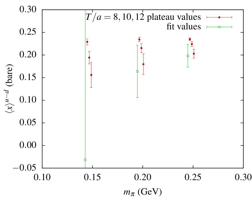
Figure 2: Isovector average momentum fraction $\langle x\rangle^{u-d}$ (bare) versus $m_{\pi}$ (GeV). At each pion mass, from left to right are results obtained from the fitting procedure, and from the ratio method with three increasing source-sink separations.

4 Fit results

We perform 2-state fits to compute $(r_{1}^{u-d})^{2}$. This involves fitting to $C_{\text{2pt}}$ and $C_{\text{3pt}}^{V^{\mu}_{u-d}}$, and the relevant (transition) form-factors are defined by [13]:

$$\langle N_{n^{\prime}}(p^{\prime},\lambda^{\prime})|V^{\mu}|N_{n}(p,\lambda)\rangle=\bar{u}_{n^{\prime}}(p^{\prime},\lambda^{\prime})\left[\left(\delta^{\mu}_{\nu}-\frac{\Delta^{\mu}\Delta_{\nu}}{\Delta^{2}}\right)\gamma^{\nu}F_{1}^{n\to n^{\prime}}(t)+\frac{i\sigma^{\mu\alpha}\Delta_{\alpha}}{m_{n}+m_{n^{\prime}}}F_{2}^{n\to n^{\prime}}(t)\right]u_{n}(p,\lambda),$$

where $\Delta=p^{\prime}-p$. Combining 3-point functions that (up to an overall sign) have the same set of contributions from form-factors, at the first nonzero momentum transfer there are three independent $C_{\text{3pt}}^{V^{\mu}}(T,\tau)$, which correspond to the three matrix elements listed in Fig. 3. Including these in a fit with the three-point functions at zero momentum transfer (both at rest and boosted), for $\tau/a\in[1,T/a-1]$, $T/a\in\{8,10,12\}$, and with $C_{\text{2pt}}(T,\vec{p})$, for $\vec{p}\in\{0,\tfrac{2\pi}{L}(1,0,0)\}$ and $T/a\in[2,12]$, we arrive at a fit to 211 variables, with 20 linear fit parameters and 3 mass parameters $m_{0}$, $m_{1}^{(2)}$, and $m_{1}^{(3)}$. As before, the Dirac radius is determined using a linear fit to the resulting $F_{1}(0)$ and $F_{1}(t_{1})$.

Selected parameters and derived quantities from the fit to the $m_{\pi}=250$ MeV ensemble are shown in Tab. 1. In particular, note that the best-fit excited-state mass for the three-point function is lower than that for the two-point function. This suggests that there may be a state that has important contributions to three-point functions but is not easily detected from the two-point function of a single smeared nucleon operator. The fit model is compared with the 3-point functions at the first nonzero momentum transfer and $T/a=8$ in Fig. 3. In this figure, contributions from the ground-state nucleon will decay approximately as $\exp(-0.03\tau/a)$, since the nucleon with nonzero momentum at the source has slightly higher energy than the nucleon at rest at the sink. This is the approximate behavior seen in the first two of the three 3-point functions, however the third approaches zero more rapidly. This can be explained if the different three-point functions have different relative contributions from excited states. This is extra information that the fit is able to make use of, but is discarded when producing a plateau plot.

In Fig. 2, we compare $(r_{1}^{u-d})^{2}$ from this fit with the values from the ratio method. The fit results show a stronger trend of increasing Dirac radius at smaller pion masses, although since the fit points have large errors (only slightly smaller than for the $T/a=12$ plateau values), the outcome from the fit is consistent with with the $T/a=10$ plateau values across all ensembles.

$\chi^{2}/\text{dof}$	89(22)/188
$\lambda$	0.036(12)
$m_{0}a$	0.637(6)
$m_{1}^{(2)}a$	1.55(14)
$m_{1}^{(3)}a$	0.99(5)
$a_{n}(0,0,0)$	$\begin{pmatrix}2.41(9)\\ 2.87(47)\end{pmatrix}\times 10^{-10}$
$a_{n}(\tfrac{2\pi}{L},0,0)$	$\begin{pmatrix}2.08(8)\\ 2.49(41)\end{pmatrix}\times 10^{-10}$
$\tilde{F}_{1}^{n\to n^{\prime}}(t_{1})$	$\begin{pmatrix}2.09(9)&-0.18(5)\\ -0.21(4)&-0.23(27)\end{pmatrix}\times 10^{-10}$
$\tilde{F}_{2}^{n\to n^{\prime}}(t_{1})$	$\begin{pmatrix}7.3(5)&-0.7(2)\\ -0.5(3)&-11.1(7.4)\end{pmatrix}\times 10^{-10}$
$F_{1}(t_{1})$	0.934(10)
$F_{2}(t_{1})$	3.25(13)

Table 1: Selected results from fit used to compute $(r_{1}^{u-d})^{2}$ for the $m_{\pi}=250$ MeV ensemble. Form-factors $F_{1,2}(t_{1})$ are not renormalized and are computed from $\tilde{F}_{1,2}^{0\to 0}(t_{1})\!\bigg{/}\!\!\sqrt{a_{0}(0,0,0)a_{0}(\tfrac{2\pi}{L},0,0)}$.

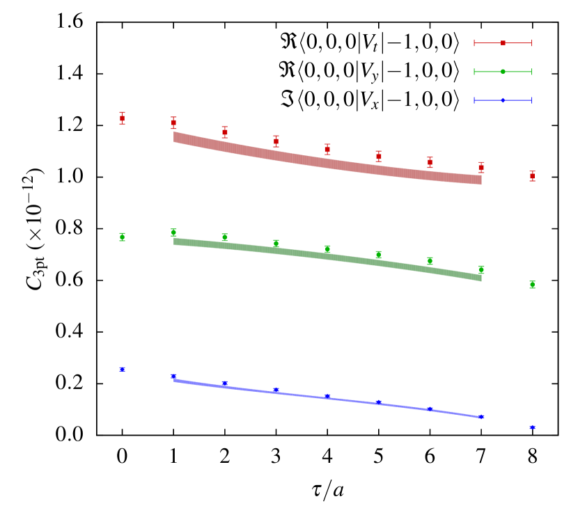
Figure 3: Three-point function (points) and fit (error bands) versus $\tau/a$, with $T/a=8$. Matrix element labels are representatives from the sets of equivalent three-point functions that are averaged to compute the points shown here. Fit bands are determined by the quantities $m_{0}a$, $m_{1}^{(3)}a$, $\tilde{F}_{1}(t_{1})$, and $\tilde{F}_{2}(t_{2})$ listed in Tab. 1. Note that the points have correlated errors, and that neglecting correlations will cause the fit to overlap with the data.

To determine $\langle x\rangle^{u-d}$, we perform the analogous fit to $C_{\text{2pt}}$ and $C_{\text{3pt}}^{\mathcal{O}^{\mu\nu}_{u-d}}$, except that we restrict to $\tau/a\in[2,T/a-2]$, since the operator extends in the time direction. The (transition) matrix elements are parametrized by five generalized form-factors:

$$\langle N_{n^{\prime}}(p^{\prime},\lambda^{\prime})|\mathcal{O}^{\{\mu\nu\}}|N_{n}(p,\lambda)\rangle =\bar{u}_{n^{\prime}}(p^{\prime},\lambda^{\prime})\biggl{[}\bar{p}^{\{\mu}\gamma^{\nu\}}A_{20}^{n\to n^{\prime}}(t)+\Delta^{\{\mu}\gamma^{\nu\}}A_{21}^{n\to n^{\prime}}(t)$$

$$\qquad\qquad+\bar{p}^{\{\mu}\frac{i\sigma^{\nu\}\alpha}\Delta_{\alpha}}{m_{n}+m_{n^{\prime}}}B_{20}^{n\to n^{\prime}}(t)+\Delta^{\{\mu}\frac{i\sigma^{\nu\}\alpha}\Delta_{\alpha}}{m_{n}+m_{n^{\prime}}}B_{21}^{n\to n^{\prime}}(t)$$

$$\qquad\qquad+\frac{2}{m_{n}+m_{n^{\prime}}}\Delta^{\{\mu}\Delta^{\nu\}}C_{2}^{n\to n^{\prime}}(t)\biggr{]}u_{n}(p,\lambda),$$

where $\bar{p}=(p^{\prime}+p)/2$, and $A_{21}$ and $B_{21}$ vanish for non-transition matrix elements due to time-reversal symmetry [14]. Including the first nonzero momentum transfer helps to give a better handle on the excited-state mass. Overall, the fit has 358 variables, with 38 linear fit parameters and the three masses. The fit results for $\langle x\rangle^{u-d}\equiv A_{20}(0)$ are compared with the ratio method in Fig. 2. These show the same downward trend as the pion mass decreases that was seen in the $T/a=10,12$ plateau values, but with larger errors. At $m_{\pi}=150$ MeV, statistics were too poor, such that the value obtained from the fit, $\langle x\rangle^{u-d}=-0.03(67)$, is not useful.

5 Conclusion

There is strong evidence of excited-state contamination in nucleon structure calculations. We see that the effect depends on the observable and consequently there is a clear need to quantify the systematic error from excited states for each observable. In particular, as demonstrated in Fig. 2, the use of a single source-sink separation smaller than about 1.4 fm is inadequate for accurate calculations of the isovector average momentum fraction near the physical pion mass.

We have presented one promising approach to reducing this problem by including an additional finite number of excited states in a fit. Applying this method with one excited state, we obtain results that, with currently available statistics, are consistent with the ratio method.

- [1] C. Alexandrou, Hadron Structure and Form Factors, PoS LATTICE2010 (2010) 001 [1011.3660].
- [2] D. B. Renner, Status of Average-x from Lattice QCD, AIP Conf. Proc. 1369 (2011) 29–36 [1103.3655].
- [3] S. Capitani, B. Knippschild, M. Della Morte and H. Wittig, Systematic errors in extracting nucleon properties from lattice QCD, PoS LATTICE2010 (2010) 147 [1011.1358].
- [4] B. Brandt et. al., Form factors in lattice QCD, Eur. Phys. J. ST 198 (2011) 79–94 [1106.1554].
- [5] J. D. Bratt et. al., Nucleon structure from mixed action calculations using 2+1 flavors of asqtad sea and domain wall valence fermions, Phys. Rev. D82 (2010) 094502 [1001.3620].
- [6] O. Ledoit and M. Wolf, A well-conditioned estimator for large-dimensional covariance matrices, Journal of Multivariate Analysis 88 (2004), no. 2 365–411.
- [7] J. Schäfer and K. Strimmer, A Shrinkage Approach to Large-Scale Covariance Matrix Estimation and Implications for Functional Genomics, Statistical Applications in Genetics and Molecular Biology 4 (2005), no. 1 32.
- [8] B. C. Tiburzi, Time Dependence of Nucleon Correlation Functions in Chiral Perturbation Theory, Phys. Rev. D80 (2009) 014002 [0901.0657].
- [9] S. Dürr et. al., Lattice QCD at the physical point: Simulation and analysis details, JHEP 08 (2011) 148 [1011.2711].
- [10] S. Dinter et. al., Precision Study of Excited State Effects in Nucleon Matrix Elements, Phys. Lett. B704 (2011) 89–93 [1108.1076].
- [11] R. G. Edwards et. al., Nucleon structure in the chiral regime with domain wall fermions on an improved staggered sea, PoS LAT2006 (2006) 121 [hep-lat/0610007].
- [12] Ph. Hägler et. al., Nucleon Generalized Parton Distributions from Full Lattice QCD, Phys. Rev. D77 (2008) 094502 [0705.4295].
- [13] H.-W. Lin and S. D. Cohen, Roper Properties on the Lattice: An Update, 1108.2528.
- [14] M. Diehl, Generalized parton distributions, Phys. Rept. 388 (2003) 41–277 [hep-ph/0307382].