On an iteration leading to a $q$-analogue of the Digamma function

Abstract

We show that the $q$-Digamma function $\psi_{q}$ for $0<q<1$ appears in an iteration studied by Berg and Durán. In addition we determine the probability measure $\nu_{q}$ with moments $1/\sum_{k=1}^{n+1}(1-q)/(1-q^{k})$, which are $q$-analogues of the reciprocals of the harmonic numbers.

2010 Mathematics Subject Classification: primary 33D05; secondary 44A60.

Keywords: $q$-digamma function, Hausdorff moment sequence, p-function.

1 Introduction

For a measure $\mu$ on the unit interval $[0,1]$ we consider its Bernstein transform

$$\mathcal{B}(\mu)(z)=\int_{0}^{1}\frac{1-t^{z}}{1-t}d\mu(t),\quad\Re z>0,$$ (1)

as well as its Mellin transform

$$\mathcal{M}(\mu)(z)=\int_{0}^{1}t^{z}d\mu(t),\quad\Re z>0.$$ (2)

These functions are clearly holomorphic in the right half-plane $\Re z>0$.

The two integral transformations are combined in the following theorem from [3] about Hausdorff moment sequences, i.e., sequences $(a_{n})_{n\geq 0}$ of the form

$$a_{n}=\int_{0}^{1}t^{n}\,d\mu(t),$$ (3)

for a positive measure $\mu$ on the unit interval.

Theorem 1.1

Let $(a_{n})_{n\geq 0}$ be a Hausdorff moment sequence as in (3) with $\mu\neq 0$. Then the sequence $(T(a_{n}))_{n\geq 0}$ defined by $T(a_{n})_{n}=1/(a_{0}+\ldots+a_{n})$ is again a Hausdorff moment sequence, and its associated measure $\widehat{T}(\mu)$ has the properties $\widehat{T}(\mu)(\{0\})=0$ and

$$\mathcal{B}(\mu)(z+1)\mathcal{M}(\widehat{T}(\mu))(z)=1\quad\mbox{for}\quad\Re z>0.$$ (4)

This means that the measure $\widehat{T}(\mu)$ is determined as the inverse Mellin transform of the function $1/\mathcal{B}(\mu)(z+1)$.

It follows by Theorem 1.1 that $T$ maps the set of normalized Hausdorff moment sequences (i.e., $a_{0}=1$) into itself. By Tychonoff’s extension of Brouwer’s fixed point theorem, $T$ has a fixed point $(m_{n})$. Furthermore, it is clear that a fixed point $(m_{n})$ is uniquely determined by the equations

$$(1+m_{1}+\ldots+m_{n})m_{n}=1,\quad n\geq 1.$$ (5)

Therefore

$$m_{n+1}^{2}+\frac{m_{n+1}}{m_{n}}-1=0,$$ (6)

giving

$$m_{1}=\frac{-1+\sqrt{5}}{2},\quad m_{2}=\frac{\sqrt{22+2\sqrt{5}}-\sqrt{5}-1}{4},\ldots\,.$$

Similarly, $\widehat{T}$ maps the set $M_{+}^{1}([0,1])$ of probability measures on $[0,1]$ into itself. It has a uniquely determined fixed point $\omega$ and

$$m_{n}=\int_{0}^{1}t^{n}\,d\omega(t),\quad n=0,1,\ldots.$$ (7)

Berg and Durán studied this fixed point in [4],[5], and it was proved that the Bernstein transform $f=\mathcal{B}(\omega)$ is meromorphic in the whole complex plane and characterized by a functional equation and a log-convexity property in analogy with Bohr-Mollerup’s characterization of the Gamma function. Let us also mention that $\omega$ has an increasing and convex density with respect to Lebesgue measure $m$ on the unit interval.

An important step in the proof is to establish that $\omega$ is an attractive fixed point so that in particular the iterates $\widehat{T}^{\circ n}(\delta_{1})$ converge weakly to $\omega$. Here and in the following $\delta_{a}$ denotes the Dirac measure with mass 1 concentrated in $a\in\mathbb{R}$.

It is easy to see that $\widehat{T}(\delta_{1})=m$, because

$$T(1,1,\ldots)_{n}=\frac{1}{n+1}=\int_{0}^{1}t^{n}\,dt.$$

It is well-known that the Bernstein transform of Lebesgue measure $m$ on $[0,1]$ is related to the Digamma function $\psi$, i.e., the logarithmic derivative of the Gamma function, since

$$\int_{0}^{1}\frac{1-t^{z}}{1-t}dt=\psi(z+1)+\gamma=\sum_{n=1}^{\infty}\frac{z}{n(n+z)},\quad\Re z>0,$$ (8)

cf. [9, 8.36]. Here $\gamma=-\psi(1)$ is Euler’s constant.

Therefore $\nu_{1}:=\widehat{T}(m)=\widehat{T}^{\circ 2}(\delta_{1})$ is determined by

$$\mathcal{M}(\nu_{1})(z)=\frac{1}{\mathcal{B}(m)(z+1)}=\frac{1}{\psi(z+2)+\gamma}.$$

The measure $\nu_{1}=\widehat{T}(m)$ is given explicitly in [3] as

$$\nu_{1}=(\sum_{n=0}^{\infty}\alpha_{n}t^{\xi_{n}})\,dt,$$ (9)

where $\xi_{0}=0$, $\xi_{n}\in(n,n+1),n=1,2,\ldots$ is the solution to $\psi(1-\xi_{n})=-\gamma$ and $\alpha_{n}=1/\psi^{\prime}(1-\xi_{n})$. The moments of the measure $\nu_{1}$ are the reciprocals of the harmonic numbers, i.e.,

$$\int_{0}^{1}t^{n}\;d\nu_{1}(t)=\frac{1}{\mathcal{H}_{n+1}}=\left(\sum_{k=1}^{n+1}\frac{1}{k}\right)^{-1}.$$ (10)

The purpose of this paper is to study the first elements of the sequence $\widehat{T}^{\circ n}(\delta_{q})$, where $0<q<1$ is fixed. The reason for excluding $q=0$ is that $\widehat{T}(\delta_{0})=\delta_{1}$. Since $\omega$ is an attractive fixed point, we know that the sequence converges weakly to $\omega$.

The first step in the iteration is easy:

$$\widehat{T}(\delta_{q})=(1-q)\sum_{k=0}^{\infty}q^{k}\delta_{q^{k}},$$ (11)

because

$$\int_{0}^{1}t^{z}\,d\,\widehat{T}(\delta_{q})(t)=\frac{1-q}{1-q^{z+1}}=(1-q)\sum_{k=0}^{\infty}q^{k}q^{kz}.$$ (12)

This shows that $\widehat{T}(\delta_{q})$ is the Jackson $d_{q}t$-measure on $[0,1]$ used in the theory of $q$-integrals, cf. [8]. It is a $q$-analogue of Lebesgue measure in the sense that $d_{q}t\to m$ weakly for $q\to 1$.

It is therefore to be expected that $\nu_{q}:=\widehat{T}(d_{q}t)=\widehat{T}^{\circ 2}(\delta_{q})$ is a $q$-analogue of the measure $\nu_{1}$, and we are going to determine $\nu_{q}$ as closely as possible. We have

$$\mathcal{M}(\nu_{q})(z)=\frac{1}{f_{q}(z+1)},$$ (13)

where $f_{q}$ is defined as the Bernstein transform of $d_{q}t$:

$$f_{q}(z)=\int_{0}^{1}\frac{1-t^{z}}{1-t}\,d_{q}t=(1-q)\left(z+\sum_{k=1}^{\infty}q^{k}\frac{1-q^{kz}}{1-q^{k}}\right).$$ (14)

This formula is a $q$-analogue of (8). The moments of $\nu_{q}$ are $q$-analogues of (10)

$$\int_{0}^{1}t^{n}\,d\nu_{q}(t)=\left(\sum_{k=0}^{n}\frac{1-q}{1-q^{k+1}}\right)^{-1}.$$ (15)

Our main result is the following (note that the Haar measure on the multiplicative group $]0,\infty[$ is $dt/t$):

Theorem 1.2

The measure $\nu_{q}$ has a continuous density $\widetilde{\nu_{q}}(t)$ with respect to $dt/t$ on $]0,1]$. It is $C^{\infty}$ on each of the open intervals $]q^{k+1},q^{k}[,k=0,1,\ldots$ with jump of the derivative of size $q^{k}/(1-q^{k})(1-q)$ at the point $q^{k},k=1,2,\ldots$. Furthermore, $\lim_{t\to 0}\widetilde{\nu_{q}}(t)=0$.

Remark 1.3

It follows that the behaviour of $\widetilde{\nu_{q}}(t)$ is oscillatory, and therefore quite different from that of $\lim_{q\to 1}\widetilde{\nu_{q}}(t)$, which is increasing and convex. In fact, it follows from (9) that

$$\lim_{q\to 1}\widetilde{\nu_{q}}(t)=\sum_{n=0}^{\infty}\alpha_{n}t^{\xi_{n}+1},\quad 0<t\leq 1.$$

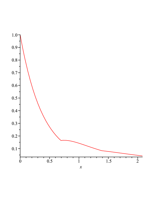
Figure 1: The graph of $(1-q)\tau_{q}$ on $[0,3\log(1/q)]$ for $q=0.5$

See Figure 1 and 2 which shows the graph of $\widetilde{\nu_{q}}(e^{-t})$ for $q=0.5$ and $q=0.9$.

2 Proofs

Jackson’s $q$-analogue of the Gamma function is defined as

$$\Gamma_{q}(z)=\frac{(q;q)_{\infty}}{(q^{z};q)_{\infty}}(1-q)^{1-z},$$

cf. [8], and its logarithmic derivative

$$\psi_{q}(z)=\frac{d}{dz}\log\Gamma_{q}(z)=-\log(1-q)+\log q\sum_{k=0}^{\infty}\frac{q^{k+z}}{1-q^{k+z}}$$ (16)

has been proposed in [11] as a $q$-analogue of the Digamma function $\psi$. See also the recent paper [12]. We define the $q$-analogue of Euler’s constant as

$$\gamma_{q}=-\psi_{q}(1)=\log(1-q)-\log q\sum_{k=1}^{\infty}\frac{q^{k}}{1-q^{k}}.$$ (17)

The Bernstein transform $f_{q}$ of $d_{q}t$ is given in (14), hence

$$\frac{f_{q}(z)}{1-q} = z+\sum_{k=1}^{\infty}q^{k}\sum_{n=0}^{\infty}q^{kn}(1-q^{kz})$$

$$= z+\sum_{n=0}^{\infty}\left(\sum_{k=1}^{\infty}(q^{k(n+1)}-q^{k(n+1+z)})\right)$$

$$= z+\frac{1}{\log(1/q)}\left(\gamma_{q}+\psi_{q}(z+1)\right),$$

which shows the close relationship with the $q$-Digamma function. We will be using another expression for $f_{q}(z)/(1-q)$ derived from (14), namely

$$\frac{f_{q}(z)}{1-q}=z+c_{q}-\sum_{k=1}^{\infty}\frac{q^{k}}{1-q^{k}}q^{kz},$$ (18)

with

$$c_{q}=\sum_{k=1}^{\infty}\frac{q^{k}}{1-q^{k}}.$$ (19)

Clearly, $q/(1-q)<c_{q}<q/(1-q)^{2}$ for $0<q<1$ and $q\mapsto c_{q}$ is a stricly increasing map of $]0,1[$ onto $]0,\infty[$. We mention two other expressions

$$c_{q}=\sum_{n=1}^{\infty}d(n)q^{n}=\sum_{n=1}^{\infty}\left(1-(q^{n};q)_{\infty}\right),$$

where $d(n)$ is the number of divisors in $n$, see [7, p. 14].

In order to replace the Mellin transformation by the Laplace transformation we introduce the probability measure $\tau_{q}$ on $[0,\infty[$ which has $\nu_{q}$ as image measure under $t\to e^{-t}$, hence

$$\mathcal{L}(\tau_{q})(z)=\int_{0}^{\infty}e^{-tz}\,d\tau_{q}(t)=\frac{1}{f_{q}(z+1)}.$$

The analogue of Theorem 1.2 about the measure $\tau_{q}$ is given in the next theorem, which we shall prove first.

Theorem 2.1

The measure $\tau_{q}$ has a continuous density also denoted $\tau_{q}$ with respect to Lebesgue measure on $[0,\infty[$. It is $C^{\infty}$ in each of the open intervals $]n\log(1/q),(n+1)\log(1/q)[,n=0,1,\ldots$ with jump of the derivative of size

$$J_{n}=\frac{q^{2n}}{(1-q^{n})(1-q)}$$ (20)

at the point $n\log(1/q),n=1,2,\ldots$. Furthermore, $\lim_{t\to\infty}\tau_{q}(t)=0$.

Proof of Theorem 2.1. Introducing the discrete measure

$$\mu=\sum_{k=1}^{\infty}\frac{q^{2k}}{1-q^{k}}\delta_{k\log(1/q)}$$

of finite total mass

$$||\mu||_{1}=c_{q}-q/(1-q)<c_{q},$$ (21)

we can write

$$\frac{f_{q}(z+1)}{1-q}=1+c_{q}+z-\mathcal{L}(\mu)(z),$$

hence

$$\frac{1-q}{f_{q}(z+1)}=\left((1+c_{q}+z)(1-\frac{\mathcal{L}(\mu)(z)}{1+c_{q}+z})\right)^{-1}=\sum_{n=0}^{\infty}\frac{\left(\mathcal{L}(\mu)(z)\right)^{n}}{\left(1+c_{q}+z\right)^{n+1}}.$$ (22)

Let $\rho_{q}$ denote the following exponential density restricted to the positive half-line

$$\rho_{q}(t)=\exp(-(1+c_{q})t)Y(t),$$

where $Y$ is the usual Heaviside function equal to 1 for $t\geq 0$ and equal to zero for $t<0$. Its Laplace transform is given as

$$\int_{0}^{\infty}e^{-tz}\rho_{q}(t)\,dt=(1+c_{q}+z)^{-1},$$

but this shows that (22) is equivalent to the following convolution equation

$$(1-q)\tau_{q}=\rho_{q}\ast\sum_{n=0}^{\infty}(\mu\ast\rho_{q})^{\ast n}=\sum_{n=0}^{\infty}\rho_{q}^{\ast(n+1)}\ast\mu^{\ast n}.$$ (23)

This equation expresses a factorization of $(1-q)\tau_{q}$ as the convolution of the exponential density $\rho_{q}$ and an elementary kernel $\sum_{0}^{\infty}N^{\ast n}$ with $N=\mu\ast\rho_{q}$. For information about the basic notion of elementary kernels in potential theory, see [6, p.100]. All three measures in question $\tau_{q},\rho_{q}$ and $\sum_{0}^{\infty}(\mu\ast\rho_{q})^{\ast n}$ are potential kernels on $\mathbb{R}$ in the sense of [6].

The measure $\mu^{\ast n},n\geq 1$ is a discrete measure concentrated in the points $k\log(1/q),k=n,n+1,\ldots$. The convolution powers of $\rho_{q}$ are Gamma densities

$$\rho_{q}^{\ast(n+1)}(t)=\frac{t^{n}}{n!}e^{-(1+c_{q})t}Y(t),$$

as is easily seen by Laplace transformation.

Clearly, $\rho_{q}\ast\mu$ is a bounded integrable function with

$$||\rho_{q}\ast\mu||_{\infty}\leq||\rho_{q}||_{\infty}||\mu||_{1}<c_{q},\quad||\rho_{q}\ast\mu||_{1}=||\rho_{q}||_{1}||\mu||_{1}<\frac{c_{q}}{1+c_{q}},$$ (24)

and then $\rho_{q}\ast(\rho_{q}\ast\mu)^{\ast n},n\geq 1$ is a continuous integrable function on $\mathbb{R}$, vanishing for $t\leq n\log(1/q)$ and for $t\to\infty$. Furthermore,

$$||\rho_{q}\ast(\rho_{q}\ast\mu)^{\ast n}||_{\infty}<(c_{q}/(1+c_{q}))^{n},$$

and this shows that the right-hand side of (23) converges uniformly on $[0,\infty[$, so $(1-q)\tau_{q}$ has a continuous density on $[0,\infty[$ tending to 0 at infinity.

For $n\geq 1$ and $x\in[n\log(1/q),\infty[$ we get

$$\rho_{q}^{\ast(n+1)}\ast\mu^{\ast n}(x)$$

$$= \int_{0}^{x}\frac{(x-t)^{n}}{n!}e^{-(1+c_{q})(x-t)}Y(x-t)\,d\mu^{\ast n}(t)$$

$$= e^{-(1+c_{q})x}\sum_{k=n}^{\infty}\frac{(x-k\log(1/q))^{n}}{n!}q^{-k(1+c_{q})}Y(x-k\log(1/q))\mu^{\ast n}(k\log(1/q))$$

which is a finite sum, and

$$\mu^{\ast n}(k\log(1/q))=\sum_{p_{1}+\ldots+p_{n}=k}\prod_{j=1}^{n}\frac{q^{2p_{j}}}{1-q^{p_{j}}},\;k=n,n+1,\ldots.$$

In particular,

$$\mu^{\ast n}(n\log(1/q))=\left(\frac{q^{2}}{1-q}\right)^{n}.$$

For $n\geq 0$ and $0\leq x<(n+1)\log(1/q)$ we then get

$$(1-q)\tau_{q}(x)=$$

$$e^{-(1+c_{q})x}\sum_{j=0}^{n}q^{-j(1+c_{q})}Y(x-j\log(1/q))\sum_{k=0}^{j}\frac{(x-j\log(1/q))^{k}}{k!}\mu^{\ast k}(j\log(1/q)).$$

On $[0,\log(1/q)[$ it is equal to $\exp(-(1+c_{q})x)$, on $[\log(1/q),2\log(1/q)[$ it is equal to

$$\exp(-(1+c_{q})x)\left(1+\frac{q^{1-c_{q}}}{1-q}(x-\log(1/q))\right),$$

on $[2\log(1/q),3\log(1/q)[$ it is equal to

$$\exp(-(1+c_{q})x)\left(1+\frac{q^{1-c_{q}}}{1-q}(x-\log(1/q))+\right.$$

$$\left.\frac{q^{2(1-c_{q})}}{1-q^{2}}(x-2\log(1/q))+\frac{q^{2(1-c_{q})}}{2(1-q)^{2}}(x-2\log(1/q))^{2}\right),$$

etc.

Using the expression (2) it is possible to calculate the derivative of $(1-q)\tau_{q}$ from the right and from the left at the point $x=n\log(1/q),n\geq 1$. The difference between the right and the left derivative equals $q^{2n}/(1-q^{n})$ and this gives the jump $J_{n}$ of (20). $\square$

It is straightforward to transfer the results of Theorem 2.1 to give Theorem 1.2 using that $\nu_{q}$ is the image measure of $\tau_{q}$ under $t\mapsto e^{-t}$, hence $\widetilde{\nu_{q}}(t)=\tau_{q}(\log(1/t)),\;0<t\leq 1$.

Remark 2.2

The representation (22) and Theorem 2.1 show that $(1-q)\tau_{q}$ is a standard $p$-function in the terminology from the theory of regenerative phenomena, cf. [10].

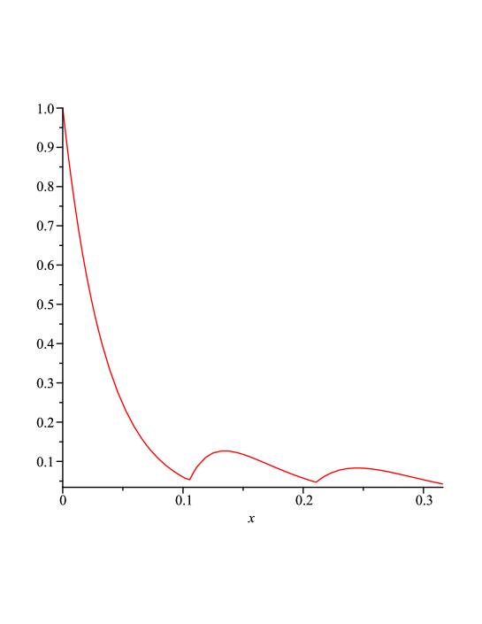
Figure 2: The graph of $(1-q)\tau_{q}$ on $[0,3\log(1/q)]$ for $q=0.9$

3 Further properties of $\tau_{q}$

Formally, by Fourier inversion we get that

$$\tau_{q}(x)=\frac{1}{2\pi}\int_{-\infty}^{\infty}e^{iyx}\frac{dy}{f_{q}(1+iy)}.$$

The function $1/f_{q}(1+iy)$ is a non-integrable $L^{2}$-function, so the formula holds in the $L^{2}$-sense. To see this we notice that

$$\frac{f_{q}(z)}{z}=1-q+\int_{0}^{\infty}e^{-tz}h_{q}(t)\,dt,\quad\Re z>0,$$

where

$$h_{q}(t)=(1-q)\sum_{k>t/\log(1/q)}\frac{q^{k}}{1-q^{k}}.$$ (26)

In particular

$$\frac{f_{q}(1+iy)}{1+iy}=1-q+\int_{0}^{\infty}e^{-ity}e^{-t}h_{q}(t)\,dt,$$

and since $e^{-t}h_{q}(t)$ is integrable, it follows from the Riemann-Lebesgue Lemma that we get the asymptotic behaviour

$$f_{q}(1+iy)\sim(1-q)(1+iy),\quad|y|\to\infty.$$ (27)

Furthermore, we notice that

$$\Re f_{q}(1+iy)=1-q+(1-q)\sum_{k=1}^{\infty}\frac{q^{k}}{1-q^{k}}\left(1-q^{k}\cos(ky\log(q))\right),$$

hence

$$1\leq\Re f_{q}(1+iy)\leq 1-q+\sum_{k=1}^{\infty}q^{k}(1+q^{k}),$$

showing that $\Re f_{q}(1+iy)$ is bounded below and above. It follows that the symmetrized density

$$\varphi_{q}(x)=\begin{cases}\displaystyle\tau_{q}(x)&\text{if $x\geq 0$},\\ &\\ \displaystyle\tau_{q}(-x)&\text{if $x<0$},\end{cases}$$ (28)

is the Fourier transform of the non-negative integrable function

$$\frac{2\Re f_{q}(1+iy)}{|f_{q}(1+iy)|^{2}},$$

and therefore $\varphi_{q}(x)$ is continuous and positive definite, so $\tau_{q}$ is the restriction to $[0,\infty[$ of such a function.

Remark 3.1

The function $f_{q}$ defined in (14) is a Bernstein function in the sense of [6], but not a complete Bernstein function in the sense of [13], because $f_{q}(z)/z$ is not a Stieltjes function as shown by formula (26). This is in contrast to

$$\lim_{q\to 1}f_{q}(z)=\psi(z+1)+\gamma,$$

which is a complete Bernstein function, cf. [3].

4 Relation to other work

The transformation $T$ can be extended from normalized Hausdorff moment sequences to the set $\mathcal{K}=[0,1]^{\mathbb{N}}$ of sequences $(x_{n})=(x_{n})_{n\geq 1}$ of numbers from the unit interval $[0,1]$. This was done in [2], where $T:\mathcal{K}\to\mathcal{K}$ is defined by

$$(T(x_{n}))_{n}=\frac{1}{1+x_{1}+\ldots+x_{n}},\quad n\geq 1.$$ (29)

The connection is that a normalized Hausdorff moment sequence $(a_{n})_{n\geq 0}$ is considered as the element $(a_{n})_{n\geq 1}\in\mathcal{K}$.

Since $T$ is a continuous transformation of the compact convex set $\mathcal{K}$ in the space $\mathbb{R}^{\mathbb{N}}$ of real sequences equipped with the product topology, it has a fixed point by Tychonoff’s theorem, and this is $(m_{n})_{n\geq 1}$.

There is no reason a priori that the fixed point $(m_{n})$ of (29) should be a Hausdorff moment sequence, but as we have seen above, the motivation for the study of $T$ comes from the theory of Hausdorff moment sequences.

Although $T$ is not a contraction on $\mathcal{K}$ in the natural metric

$$d((a_{n}),(b_{n}))=\sum_{n=1}^{\infty}2^{-n}|a_{n}-b_{n}|,\quad(a_{n}),(b_{n})\in\mathcal{K},$$

it was proved in [2] that $T$ maps $\mathcal{K}$ into the compact convex subset

$$\mathcal{C}=\left\{(a_{n})\in\mathcal{K}\mid a_{1}\geq\tfrac{1}{2}\right\},$$

and the restriction of $T$ to $\mathcal{C}$ is a contraction. It is therefore possible to infer that $(m_{n})$ is an attractive fixed point from the fixed point theorem of Banach.

Christian Berg, Helle Bjerg Petersen
Department of Mathematical Sciences
University of Copenhagen
Universitetsparken 5
DK-2100 København Ø, Denmark
E-mail addresses: berg@math.ku.dk (C. Berg)
hellebp@gmail.com (H. B. Petersen).

References

• [1] Akhiezer, N.Β  I., The classical moment problem. Oliver and Boyd, Edinburgh, 1965.
• [2] Berg, C., Beygmohammadi, M., On a fixed point in the metric space of normalized Hausdorff moment sequences, Rend. Circ. Mat. Palermo, Serie II, Suppl. 82 (2010), 251–257.
• [3] Berg, C., DurΓ‘n, A. J., Some transformations of Hausdorff moment sequences and Harmonic numbers, Canad. J. Math. 57 (2005), 941–960.
• [4] Berg, C., DurΓ‘n, A. J., The fixed point for a transformation of Hausdorff moment sequences and iteration of a rational function, Math. Scand. 103 (2008), 11–39.
• [5] Berg, C., DurΓ‘n, A. J., Iteration of the rational function $z-1/z$ and a Hausdorff moment sequence, Expo. Math. 26 (2008), 375–385.
• [6] Berg, C., Forst, G., Potential theory on locally compact abelian groups. Ergebnisse der Mathematik und ihrer Grenzgebiete Band 87. Springer-Verlag, Berlin-Heidelberg-New York, 1975.
• [7] Fine, N. J., Basic hypergeometric series and applications. American Mathematical Society, Providence, RI, 1988.
• [8] Gasper, G., Rahman, M, Basic hypergeometric series. Cambridge University Press, Cambridge 1990, second edition 2004.
• [9] Gradshteyn, I. S., Ryzhik, I. M., Table of integrals, series and products, Sixth Edition, Academic Press, New York, 2000.
• [10] Kingman, J. F. C., Regenerative Phenomena. John Wiley & Sons Ltd., London 1972.
• [11] Krattenthaler, C., Srivastava, H. M., Summations for Basic Hypergeometric Series Involving a $q$-analogue of the Digamma Function, Computers Math. Applic. 32 (1996), 73–91.
• [12] Mansour, T., Shabani, A. S., Some inequalities for the $q$-Digamma function, J. Inequal. Pure and Appl. Math. 10 (2009), Art. 12, 8 pp.
• [13] Schilling, R., Song, R. and Vondraček, Z., Bernstein functions: Theory and Applications, de Gruyter, Berlin 2010.