Effects of Anisotropy in (2+1)-dimensional QED

Abstract

We summarize our results for the impact of anisotropic fermionic velocities in (2+1)-dimensional QED on the critical number of fermion flavors, $N^{c}_{f}$, and dynamical mass generation. We apply different approximation schemes for the gauge boson vacuum polarization and the fermion-boson vertex to analyze the according Dyson–Schwinger equations in a finite volume. Our results point towards large variations of $N^{c}_{f}$ away from the isotropic point in agreement with other approaches.

1 Introduction

Investigating strongly coupled theories has been a subject of great interest for many years. Amongst others, strong $\mbox{QED}_{3}$ attracted a respectable amount of attention since it provides a comparably simple environment in which to study a variety of strong coupling phenomena. However, $\mbox{QED}_{3}$ does not only serve as a test bed for investigations of more complicated theories. Viewed as a low-energy effective theory it has applications to condensed matter systems such as high-temperature superconductors (HTSs) or graphene. This strongly suggests that we need to further elaborate its understanding. In the case of HTSs, it was argued [1, 2] that the transition from the antiferromagnetic to the pseudogap phase can be described by $\mbox{QED}_{3}$. The transition between both phases is then indicated by the generation of a dynamical mass for the fermionic quasi-particles in the anti-ferromagnetic phase, whereas the pseudogap phase is chirally symmetric. The generation of such a mass term results from interactions of the fermionic quasi-particles with topological excitations that can be molded into the U(1) gauge fields of $\mbox{QED}_{3}$. Experimental observations furthermore suggest the inclusion of anisotropic fermionic velocities in the theoretical description, which can be realized in the form of a constant, but non-trivial “metric” in the Lagrangian. While there have been extensive discussions on the critical number of fermion flavors for chiral symmetry breaking in isotropic $\mbox{QED}_{3}$ both in the continuum [1, 2, 3, 4, 5, 6] and at finite volume [7, 8, 9, 10], only few results are known which consider small [11] or large anisotropies [12, 13, 14]. In this proceedings contribution, we summarize the results of our investigation of $\mbox{QED}_{3}$ with (large) anisotropic velocities, obtained within the framework of Dyson–Schwinger equations on a compact manifold [15]. First, we discuss some technical details concerning the underlying equations and introduce the approximation schemes that we use later on. In section 3 we present our results and compare them with findings within different approaches.

2 Technical Details

2.1 The Dyson–Schwinger equations in anisotropic $\mbox{QED}_{3}$

Motivated by the application of $\mbox{QED}_{3}$ as a low-energy effective theory of high-temperature superconductors, we will investigate the anisotropic theory as formulated and extensively discussed in Refs. [1, 11, 12]. Hence, we will here focus on the more important aspects of this formulation of $\mbox{QED}_{3}$. We begin with the Lagrangian for anisotropic, (2+1)-dimensional QED containing $N_{f}\,$ fermion flavors in a four dimensional spinor representation

$$\mathcal{L}^{aniso}=\frac{N_{f}}{2}\sum_{j=1,2}\bar{\Psi}_{j}\left\{\sum_{\mu=0}^{2}\gamma_{\nu}\sqrt{g}_{j,\nu\mu}\left(\partial_{\mu}+\mbox{i}\;a_{\mu}\right)\right\}\Psi_{j}.$$ (1)

The fermionic spinors obey the Clifford algebra $\{\gamma_{\mu},\gamma_{\nu}\}=2\,\delta_{\mu\nu}$.
Furthermore, the Lagrangian Eq. (1) contains the “nodal” sum $\sum_{j=1,2}$ and the – closely related – metric-like factor $g_{j,\mu\nu}$. The sum arises from the HTS-inherent d-wave symmetry of the energy gap function, that leads to in total four zeroes (the “nodes”) that are found to lie on the Fermi surface. Two of these are related by symmetry and can be grouped in pairs which are then distinguished by their nodal index $j$. Fermionic excitations close to the zeroes of the energy gap function introduce the fermionic velocities $v_{F}\,$ and $v_{\Delta}\,$ that are collected in the metric-like factor $g_{j,\mu\nu}$ defined as

$$\left(g_{1}^{\mu\nu}\right)=\left(\begin{array}[]{ccc}1&0&0\\ 0&\,v_{F}\,^{2}&0\\ 0&0&v_{\Delta}\,^{2}\end{array}\right)$$

$$\left(g_{2}^{\mu\nu}\right)=\left(\begin{array}[]{ccc}1&0&0\\ 0&v_{\Delta}\,^{2}&0\\ 0&0&v_{F}\,^{2}\end{array}\right).$$ (2)

In the following, we will investigate the breaking of chiral symmetry that reduces the original symmetry of the Lagrangian to $\;U(2N_{f})\rightarrow\;SU(N_{f})\times SU(N_{f})\times U(1)\times U(1)\;$, when the fermions obtain dynamically generated mass terms. The order parameter of the chiral phase transition is given by the chiral condensate that can be determined from the trace of the fermionic propagator $S_{F,j}(\vec{p})$.

The diagrammatic representation of the corresponding Dyson–Schwinger equations for the fermion propagator $S_{F,i}$ and the bosonic propagator $D_{\mu\nu}$ are displayed in Fig. 1. In Euclidean space-time, they are denoted as

$$S_{F,i}^{-1}(\vec{p}\;)\; = S_{0}^{-1}(\,\vec{p}\,)\;\;+\,Z_{1}\,e^{2}\int\frac{d^{3}q}{(2\pi)^{3}}(\sqrt{g}_{i,\mu\alpha}\gamma^{\alpha}\,S_{F,i}(\,\vec{q}\,)\,\sqrt{g}_{i,\nu\beta}\Gamma^{\beta}(\,\vec{q},\vec{p}\,)\,D_{\mu\nu}(\,\vec{k}\,)),$$ (3)

$$D_{\mu\nu}^{-1}(\vec{p}\;) = D_{0,\mu\nu}^{-1}(\,\vec{p}\,)-Z_{1}\,e^{2}\,\frac{N_{f}}{2}\,\sum_{i=1,2}\int\frac{d^{3}q}{(2\pi)^{3}}\mbox{Tr}\left[\sqrt{g}_{i,\mu\alpha}\gamma^{\alpha}\,S_{F,i}(\,\vec{q}\,)\;\sqrt{g}_{i,\nu\beta}\Gamma^{\beta}(\,\vec{p},\vec{q}\,)\,S_{F,i}(\,\vec{k}\,))\right],$$ (4)

with the momentum $\,\vec{k}\,$ defined as the difference $\vec{p}-\vec{q}$ and $i=1,2$. Here, the renormalization constant $Z_{1}$ of the fermion-boson vertex, $\,\Gamma^{\beta}(\,\vec{p},\vec{q}\;)$, is included.

Figure 1: The diagrammatic representation of the Dyson–Schwinger equations for the fermion (lhs) and gauge boson propagator (rhs). Wiggly lines denote photon propagators, straight lines fermion propagators. A blob denotes a dressed propagator or vertex, whereas a dot stands for a bare fermion-photon vertex.

We introduce several shorthands in order to keep track of the structure of the equations during further discussion. These are

$$\overline{p}_{i}^{2}:=p_{\mu}\;g_{i}^{\mu\nu}\;p_{\nu}$$ (5)

and

$$\widetilde{p}_{\mu,i}:=A_{\mu,i}\left(\vec{p}\;\right)p_{\mu},\mbox{ (no summation convention !), }$$ (6)

where $A_{\mu,i}$ denotes the vectorial fermionic dressing function at node $i$.
The anisotropic dressed propagators then are given as

$$S_{F,i}^{-1}\left(\vec{p}\;\right) = B_{i}\left(\vec{p}\;\right)+\mbox{i}\;\sqrt{g_{i}}^{\mu\nu}\gamma_{\nu}\;\widetilde{p}_{\mu,i},$$ (7)

$$D_{\mu\nu}\left(\vec{p}\;\right)^{{}^{-1}} = p^{2}\left(\delta_{\mu\nu}-\frac{p_{\mu}p_{\nu}}{p^{2}}\right)+\Pi_{\mu\nu}\left(\vec{p}\;\right),$$ (8)

where $B_{i}$ denotes the scalar fermion dressing function at node i and $\Pi_{\mu\nu}\left(\,\vec{p}\;\right)$ the vacuum polarization of the gauge boson field. As the free gauge bosons do not involve fermionic velocities, the bare propagator remains the isotropic one.
In order to solve the Dyson–Schwinger equations for the fermion and the gauge boson, we apply the minimal Ball-Chiu vertex construction as ansatz for the fermion-gauge boson vertex. This is given by

$$\Gamma^{\beta}_{i}(\vec{p},\vec{q})=\gamma^{\beta}\frac{A^{\beta}_{i}(\vec{p})+A^{\beta}_{i}(\vec{q})}{2}$$ (9)

where no summation convention is used and $p,q$ are the fermion and anti-fermion momenta at the vertex.

Furthermore, we approximate the gauge boson DSE in order to keep the equations manageable. We use two different approximation schemes. Firstly, we apply the large-$N_{f}\,$ approximation and secondly a more sophisticated model based on the results of Ref. [6].
The large-$N_{f}\,$ approximation has been studied intensely for the limiting case of isotropic spacetime [3, 4] and also in an expansion for small anisotropies (see Refs. [1, 11]). In this work, we are interested in the influence of large anisotropic velocities and therefore make no further approximations concerning the “metric”. Analyzing the large-$N_{f}\,$ approximation, we expect a qualitative estimate of the effects of anisotropy on the critical quantities for chiral phase transition.
The vacuum polarization in leading order large-$N_{f}\,$ expansion is given diagrammatically in Fig. 2.

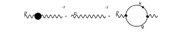
Figure 2: The diagrammatic representation of the Dyson–Schwinger equation for the vacuumpolarization of gauge bosons in leading order large-$N_{f}\,$ expansion.

After analytic integration ([1, 11]), the vacuum polarization is denoted as

$$\Pi^{\mu\nu}\left(\vec{p}\;\right) = \sum_{i}\sqrt{\overline{p}_{i}^{2}}\left(g_{i}^{\mu\nu}-\frac{g_{i}^{\mu\alpha}p_{\alpha}\;g_{i}^{\nu\delta}p_{\delta}}{\overline{p}_{i}^{2}}\right)\,\,\Pi_{i}\left(\vec{p}\;\right).$$

$$\Pi_{i}\left(\vec{p}\;\right) = \frac{e^{2}\,N_{f}}{16\,v_{F}v_{\Delta}}\frac{1}{\sqrt{\overline{p}_{i}^{2}}}.$$ (10)

Although the large-$N_{f}\,$ approximation is a good starting point to obtain first insights, it is well known that it contains several drawbacks. The origin of these lie in the fact that within a consistent large-$N_{f}\,$ approximation, the fermionic vector dressing function is independent of momentum, $A_{i,\mu}\equiv 1$. This momentum independence is in contrast to the power-law behaviour found in the infrared for the fermionic vector dressing function, the vacuum polarization and the vertex (see Ref. [6]). Moreover, the components of the vector dressing function provide for the renormalized fermionic anisotropic velocities ($c^{R}_{s},v^{R}_{f},v^{R}_{\Delta}$), which, in the general definition, would remain trivial for $A_{i,\mu}\equiv 1$. It is not intuitively clear if or how their definition can be adjusted to be consistent with the large-$N_{f}\,$ approximation. Based on the results obtained in isotropic spacetime, we go beyond large-$N_{f}\,$ by applying a generalized gauge boson model that includes the anomalous dimension $\kappa$. We extracted the anomalous dimension in the isotropic limit with a value of $\kappa=0.035$ and assume that we can neglect possible dependencies on the anisotropic velocities in this first and exploratory analysis. The improved vacuum polarization model reads

$$\Pi_{i}\left(\vec{p}\;\right)=\frac{e^{2}N_{f}}{16\,v_{F}v_{\Delta}}\left(\frac{1}{\sqrt{\overline{p}_{i}^{2}}}\frac{\overline{p}_{i}^{2}}{\overline{p}_{i}^{2}+e^{2}}+\frac{1}{\overline{p}_{i}^{1+2\kappa}}\frac{e^{2}}{{\overline{p}_{i}}^{2}+e^{2}}\right),$$ (11)

with $\overline{{p}_{i}}^{2}$ defined in Eq. (5). With the approximation schemes at hand, we proceed to the fermionic DSEs by taking the appropriate traces of Eq. (7). We obtain

$$B_{i}\left(\vec{p}\;\right) = Z_{2}\;e^{2}\int\frac{d^{3}q}{\left(2\pi\right)^{3}}\,\,\frac{B_{i}\left(\vec{q}\;\right)g_{i}^{\mu\nu}D_{\mu\nu}(\vec{k}\;)}{B_{i}\left(\vec{q}\;\right)^{2}+(\overline{\widetilde{\vec{q}}}_{i}\;)^{2}}\,\,\,\frac{A_{\mu,i}(\vec{p})+A_{\mu,i}(\vec{q})}{2},,$$ (12)

$$A_{\mu,i}\left(\vec{p}\;\right) = Z_{2}-\frac{Z_{2}\;e^{2}}{p_{\mu}}\int\frac{d^{3}q}{\left(2\pi\right)^{3}}\,\,\frac{2\left(\widetilde{q}_{\lambda,i}\;g_{i}^{\lambda\nu}D_{\mu\nu}(\vec{k}\;)\right)-\widetilde{q}_{\mu,i}\;g_{i}^{\lambda\nu}D_{\lambda\nu}(\vec{k}\;)}{B_{i}\left(\vec{q}\;\right)^{2}+(\;\overline{\widetilde{\vec{q}}}_{i}\;)^{2}}\,\,\frac{A_{\mu,i}(\vec{p})+A_{\mu,i}(\vec{q})}{2},$$ (13)

where there is again no summation convention for the index $\mu$. Since the “metric” factors are related by symmetry, the total number of equations to be solved can be reduced to eight DSEs. Nevertheless, the number of anisotropic equations is still more than double in comparison to isotropic spacetime (three equations), as we need to take the component-wise dressing of the fermion momentum and the more complex expression for the gauge boson vacuum polarization into account.

In order to solve the Dyson-Schwinger equations self-consistently we put the system in a box with finite volume $V=L^{3}$ and (anti-)periodic boundary conditions, i.e. we work on a three-torus in coordinate space which translates to discrete momenta in momentum space [7, 16]. The details of this procedure for our anisotropic case are given in Ref.[15].

3 Results

In this section, we discuss our numerical results for the critical number of fermion flavours for chiral symmetry breaking within two approximation schemes: the large-$N_{f}\,$ approximation, including only the bare vertex, and secondly the gauge boson model including the minimal Ball-Chiu vertex construction. We determine the critical number of fermion flavors with help of the scalar fermion dressing function, evaluated at minimum momentum, which serves equally well as an order parameter as e.g. the chiral condensate.

3.1 The Large-N_f Approximation

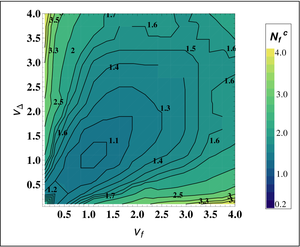
Figure 3: Critical number of fermion flavours $N_{f}^{c}$ determined in the $1/N_{f}$-approximation and plotted as a function of the fermion velocities $(v_{F}\,,v_{\Delta}\,)$.

We obtained the results for the large-$N_{f}\,$ approximations on a torus with $Le^{2}=600$ and $39^{3}$ momentum points, displayed in fig. 3. The contour lines represent the values of $N_{f}\,$, supported by a corresponding color code. Notice that the contour lines should be considered to guide the eye, as the edges in some regions result from the sparseness of our grid. In principle, we expect smooth contours in $v_{F}\,-v_{\Delta}\,-$space. For the isotropic point, ($v_{F}\,=v_{\Delta}\,=1$), we find a value of $N_{f}\,^{c}\approx 1.0$. As we expect this value to suffer from large volume effects [7], the deviation of about a factor of three from the continuum results is not surprising. Away from the isotropic point, we find increasing values for $N_{f}\,^{c}$, independent from increasing or decreasing $v_{F}\,$ and $v_{\Delta}\,$, which is in agreement with earlier Dyson–Schwinger studies of large-$N_{f}\,$ approximation and an expansion for small anisotropies [11]. Within the large-$N_{f}\,$ approximation, these results remain valid also for larger anisotropic velocities. However, as argued in the previous section, this approximation suffers from several drawbacks, which we would like to circumvent by investigation of the gauge boson model.

3.2 The Gauge Boson Model

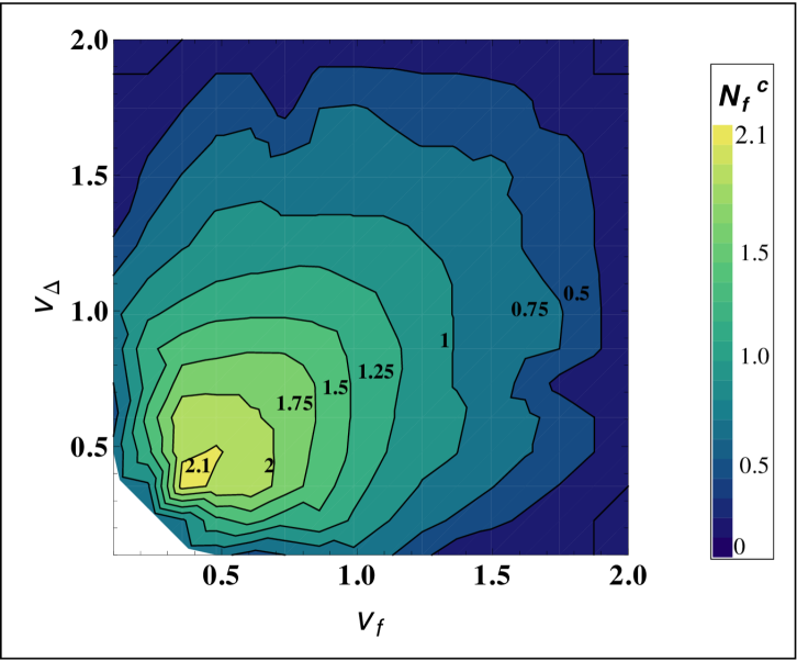
Figure 4: Critical number of fermion flavours $N_{f}^{c}$ determined from the photon model Eq. (11) and the fermion-photon vertex Eq. (9) plotted as a function of the fermion velocities $(v_{F}\,,v_{\Delta}\,)$.

The results in the gauge boson model approximation scheme are obtained on a torus with $Le^{2}=600$ and $39^{3}$ momentum points, too, and are displayed in fig. 4. The critical number of fermion flavors, $N_{f}\,^{c}$, is again indicated by contour lines and an additional color code. For the isotropic point, $v_{F}\,=v_{\Delta}\,=1$ we find $N_{f}\,^{c,model}\approx 1.1$, which is slightly different from the value obtained from large-$N_{f}\,$ approximation. Away from the isotropic point, we find a completely different behaviour of $N_{f}\,^{c}$ within our gauge boson model. We find a maximum of $N_{f}\,^{c,model}$ around $(v_{F}\,,v_{\Delta}\,)=(0.4,0.4)$ and a decreasing value of $N_{f}\,^{c,model}$ for smaller and larger anisotropies. While the critical number of fermion flavors never vanishes for $v_{F}\,,v_{\Delta}\,<1$, it reaches zero for $v_{F}\,,v_{\Delta}\,\approx 2$, meaning that the theory is always in the chirally symmetric phase. Altogether, this behaviour is in accordance with findings in the framework of a one-boson-exchange model [14] and also with lattice calculations [12, 13]. These findings, with respect to the drawbacks of large-$N_{f}\,$ approximation, leads us to the conclusion that the results from large-$N_{f}\,$ approximation are not reliable as they dismiss important features of the theory influencing the chiral phasetransition of $\mbox{QED}_{3}$.

4 Conclusions

We summarized our results of Ref. [15] using a new model for the anisotropic gauge boson vacuum polarization including characteristics that are known to be important from isotropic continuum studies of $\mbox{QED}_{3}$. We discussed the results obtained within this model in context of large-$N_{f}\,$ calculations. We found a non-vanishing critical number of fermion flavours for fermionic velocities $v_{F}\,,v_{\Delta}\,<1$ and furthermore decreasing $N_{f}\,^{c,model}$ away from a maximum around $(v_{F}\,,v_{\Delta}\,)\approx(0.4,0.4)$. These results agree qualitatively with findings from a continuum analysis of the one-boson exchange strength and with results from lattice calculations. We wish to emphasize that further investigations are necessary to quantitatively pin down the critical number of fermion flavors as a function of the velocities. Since calculations on a finite volume are necessarily hampered by large volume effects [7, 17] it seems advisable to develop further a continuum approach to the problem. Ultimately, these efforts are bound to lead to a better understanding of $\mbox{QED}_{3}$ as an effective theory of high temperature superconductors.

5 Acknowledgements

This work was supported by the Helmholtz-University Young Investigator Grant No. VH-NG-332 and by the Deutsche Forschungsgemeinschaft through SFB 634.

References

- [1] M. Franz, Z. Tesanovic and O. Vafek, Phys. Rev. B 66 (2002) 054535 [arXiv:cond-mat/0203333]; Z. Tesanovic, O. Vafek, and M. Franz, Phys. Rev. B 65 (2002) 180511 [arXiv:cond-mat/0110253]; M. Franz and Z. Tesanovic, Phys. Rev. Lett. 87, (2001) 257003. [arXiv:cond-mat/0012445];
- [2] I. F. Herbut, Phys. Rev. B 66, 094504 (2002) [arXiv:cond-mat/0202491]; Phys. Rev. Lett. 88 (2002) 047006 [arXiv:cond-mat/0110188].
- [3] T. Appelquist, D. Nash and L. C. R. Wijewardhana, Phys. Rev. Lett. 60 (1988) 2575.
- [4] D. Nash, Phys. Rev. Lett. 62 (1989) 3024.
- [5] P. Maris, Phys. Rev. D 54 (1996) 4049 [arXiv:hep-ph/9606214].
- [6] C. S. Fischer, R. Alkofer, T. Dahm and P. Maris, Phys. Rev. D 70 (2004) 073007 [arXiv:hep-ph/0407104].
- [7] T. Goecke, C. S. Fischer and R. Williams, Phys. Rev. B 79 (2009) 064513 [arXiv:0811.1887 [hep-ph]].
- [8] S. J. Hands, J. B. Kogut and C. G. Strouthos, Nucl. Phys. B 645 (2002) 321 [arXiv:hep-lat/0208030].
- [9] S. J. Hands, J. B. Kogut, L. Scorzato and C. G. Strouthos, Phys. Rev. B 70 (2004) 104501 [arXiv:hep-lat/0404013].
- [10] C. Strouthos and J. B. Kogut, arXiv:0808.2714 [cond-mat.supr-con]; C. Strouthos and J. B. Kogut, PoS LAT2007 (2007) 278 [arXiv:0804.0300 [hep-lat]].
- [11] D. J. Lee and I. F. Herbut, Phys. Rev. B 66, 094512 (2002) [arXiv:cond-mat/0201088].
- [12] S. Hands and I. O. Thomas, Phys. Rev. B 72, 054526 (2005) [arXiv:hep-lat/0412009].
- [13] I. O. Thomas and S. Hands, Phys. Rev. B 75, 134516 (2007) [arXiv:hep-lat/0609062]; PoS LAT2005, 249 (2006) [arXiv:hep-lat/0509038].
- [14] A. Concha, V. Stanev and Z. Tesanovic, Phys. Rev. B 79 (2009) 214525 [arXiv:0906.1103 [cond-mat.supr-con]].
- [15] J. A. Bonnet, C. S. Fischer, R. Williams, Phys. Rev. B 84, 024520 (2011). [arXiv:1103.1578 [hep-ph]].
- [16] C. S. Fischer, B. Gruter and R. Alkofer, Annals Phys. 321 (2006) 1918 [arXiv:hep-ph/0506053]; C. S. Fischer and M. R. Pennington, Phys. Rev. D 73 (2006) 034029 [arXiv:hep-ph/0512233]; J. Luecker, C. S. Fischer and R. Williams, Phys. Rev. D 81 (2010) 094005 [arXiv:0912.3686 [hep-ph]].
- [17] V. P. Gusynin and M. Reenders, Phys. Rev. D 68 (2003) 025017 [arXiv:hep-ph/0304302].