Revisiting the $B\to\pi\rho$, $\pi\omega$ Decays in the Perturbative QCD Approach Beyond the Leading Order

Abstract

We calculate the branching ratios and CP asymmetries of the $B\to\pi\rho$, $\pi\omega$ decays in the perturbative QCD factorization approach up to the next-to-leading-order contributions. We find that the next-to-leading-order contributions can interfere with the leading-order part constructively or destructively for different decay modes. Our numerical results have a much better agreement with current available data than previous leading-order calculations, e.g., the next-to-leading-order corrections enhance the $B^{0}\rightarrow\pi^{0}\rho^{0}$ branching ratios by a factor 2.5, which is helpful to narrow the gaps between theoretic predictions and experimental data. We also update the direct CP-violation parameters, the mixing-induced CP-violation parameters of these modes, which show a better agreement with experimental data than many of the other approaches.

I Introduction

The charmless B meson decays are not only suitable to study CP violations but also sensitive to new physicsiiba . During the past decade, the B factory experiments achieved great successes. Furthermore, the current LHC experiments will provide 2–3 orders more B meson events than the B factories lhcb1 . A large number of rare $B$ meson decay channels will be measured by the future super B factories. The research on the charmless decays of $B$ meson is therefore becoming more interesting than ever before lhcb2 .

The theoretical calculations of color-suppressed decay channels, such as $B^{0}\to\pi^{0}\pi^{0}$, met a difficulty for a relatively much smaller branching ratios than the experimental measurements prl831914 ; prd63074009 ; pdg2010 . The difference between direct CP-asymmetry measurement of $B^{0}\to K^{+}\pi^{-}$ and $B^{+}\to K^{+}\pi^{0}$ showed a very large discrepancy between the leading-order (LO) theoretical calculations and experimental data, which induced a lot of new physics discussions pikpuzzle . One of the standard model solutions to this puzzle also requires large color-suppressed tree amplitudes prd114005 . Some of the next-to-leading-order (NLO) QCD calculations in the perturbative QCD factorization approach (pQCD) prd114005 ; prd094020 ; 0807 ; prd114001 show that the NLO contributions can significantly change the LO predictions for some decay modes, especially the color-suppressed modes. It is therefore necessary to calculate the NLO corrections to those two-body charmless B meson decays in order to improve the reliability of the theoretical predictions.

The $B\to\pi\rho$ decays, which are helpful for the determination of the Cabibbo–Kobayashi–Maskawa(CKM) unitary triangle $\alpha$ angle measurement in addition to the $B\to\pi\pi$ decays, have a much more complication. Either of $B^{0}$ or $\bar{B}^{0}$ meson can decay to both the $\pi^{-}\rho^{+}$ and $\pi^{+}\rho^{-}$ final states, which lead to altogether four decay amplitudes. Since $B^{0}$ and $\bar{B}^{0}$ meson mix easily, these channels exhibit unique features of mixing and decay interference in B physics. The recent B factory measurements indeed show that the interesting phenomenology with possible large direct CP asymmetry exp . Unlike the branching ratios, the CP asymmetries are sensitive to high order contributions. Similar to the color-suppressed $B^{0}\to\pi^{0}\pi^{0}$ mode, the neutral decay modes $B^{0}\to\pi^{0}\rho^{0}$, $\pi^{0}\omega$ are also expected to receive considerable NLO contributions. Therefore, it is necessary to calculate NLO corrections to the $B\to\pi\rho,\pi\omega$ decays in the pQCD approach for the reason that previous pQCD calculations epjc23275 are already too old with only LO accuracy. In this paper, we calculate the NLO contributions arising from the vertex corrections, the quark loops and the chromo-magnetic penguin operator $O_{8g}$. Combining our results with the NLO accuracy Wilson coefficients and Sudakov suppression factors, we present a numerical analysis of $B\to\pi\rho$, $\pi\omega$ decays.

Our paper is organized as follows: we first review the pQCD factorization approach in Sec. II. Then, in Sec. III, we show our analytical results of NLO calculations. The numerical results are given in Sec. IV. Finally we close this paper with a conclusion.

II Theoretical framework

For the studied $B\to\pi\rho,\pi\omega$ decays, the weak effective Hamiltonian $\mathcal{H}_{eff}$ for $b\rightarrow d$ transition can be written as

$$\mathcal{H}_{eff}=\frac{G_{F}}{\sqrt{2}}[\xi_{u}(C_{1}(\mu)O_{1}^{u}(\mu)+C_{2}(\mu)O_{2}^{u}(\mu))-\xi_{t}\sum_{i=3}^{10}C_{i}(\mu)O_{i}(\mu)]$$ (1)

where $\xi_{u}=V_{ub}V^{*}_{ud}$, $\xi_{t}=V_{tb}V^{*}_{td}$ are the CKM matrix elements. $O_{i}(\mu)$ and $C_{i}(\mu)$ are the four-quark operators and corresponding Wilson coefficients, respectively. Expressions of $C_{i}$ and $O_{i}$ can be found in Ref.rmp681125 . In the following, we will use this effective Hamiltonian to calculate decay amplitudes in the pQCD approach. So, we first give a brief review of pQCD approach and present relevant wave functions.

II.1 pQCD factorization approach

In the framework of the pQCD factorization, three scales are involved in the non-leptonic decays of B mesons: the weak interaction scale $m_{W}$, the hard subprocess scale $t$ and the transverse momenta of the constituent quark $k_{T}$. The large logs between W boson mass scale and the hard scale $t$ have been resummed by the renormalization group equation method to give the effective Hamiltonian of four-quark operators. In two-body charmless hadronic B decays, the final state meson masses are negligible compared with the large B meson mass. Therefore the constituent quarks in the final state mesons are collinear objects in the rest frame of B meson. The momentum of light quark in B meson is at the order of $\Lambda_{QCD}$, such that a hard gluon is needed to transfer energy to make it a collinear quark into the final state meson. These perturbative calculations meet end-point singularity in dealing with the meson distribution amplitudes at the end-point. Usually in the collinear factorization approaches such as QCD factorizationprl831914 and soft-collinear effective theoryprd63114020 , people parameterize this kind of decay amplitudes into free parameters to fit the data. While in the perturbative QCD factorization approach, we take back the parton transverse momentum $k_{T}$ to regulate this divergence.

In the pQCD approach, the decay amplitude $A(B\rightarrow M_{2}M_{3})$ can be written conceptually as the convolution prd69094018

$$\mathcal{A}(B\rightarrow M_{2}M_{3})=\int d^{4}k_{1}d^{4}k_{2}d^{4}k_{3}\text{Tr}[C(t)\Phi_{B}(k_{1})\Phi_{M_{2}}(k_{2})\Phi_{M_{3}}(k_{3})H(k_{1},k_{2},k_{3},t)]$$ (2)

where $k_{i}$ are momenta of light quarks included in each meson, and Tr denotes the trace over Dirac and color indices. The hard function $H(k_{1},k_{2},k_{3},t)$ describes the four-quark operator and the spectator quark connected by a hard gluon of order $\bar{\Lambda}M_{B}$, which can be calculated perturbatively. The energy scale $t$ is chosen as the maximal virtuality of internal particles in a hard amplitude, in order to suppress higher order correctionsprd074004 . $\Phi_{M_{i}}$ is the wave function of meson $M_{i}$. The hard kernel $H$ depends on the processes considered, while the wave functions $\Phi_{M_{i}}$ are process independent that can be extracted from other well measured processes, so one can make quantitative predictions here.

It is convenient to work at the B meson rest frame and the light cone coordinate. The final state meson $M_{2}$ is moving along the direction of $v=(0,1,\bf 0_{T})$ and $M_{3}$ is along $n=(1,0,\bf 0_{T})$. Here we use $x_{i}$ to denote the momentum fractions of anti-quarks in mesons, and $\bf k_{iT}$ to denote the transverse momenta of the anti-quarks. The mass of light meson ($\pi$) is neglected. After integration over $k_{1}^{-}$, $k_{2}^{-}$ and $k_{3}^{+}$ in Eq.(2), we are led to

$$\mathcal{A} = \int dx_{1}dx_{2}dx_{3}b_{1}db_{1}b_{2}db_{2}b_{3}db_{3}$$ (3)

$$\text{Tr}[C(t)\Phi_{B}(x_{1},b_{1})\Phi_{M_{2}}(x_{2},b_{2})\Phi_{M_{3}}(x_{3},b_{3})H(x_{i},b_{i},t)S_{t}(x_{i})\exp(-S(t))]$$

where $b_{i}$ are the conjugate variables of $\bf k_{iT}$. The jet function $S_{t}(x_{i})$ arises from the threshold resummation of the large double logarithms $\ln^{2}(x_{i})$, and the Sudakov exponent $S(t)$ comes from the double logarithms of collinear and soft divergences.

II.2 Wave Functions

There are generally two Lorentz structures in the B meson distribution amplitudes, which can be decomposed as qiaocf

$$\int_{0}^{1}\frac{d^{4}z}{(2\pi)^{4}}e^{ik_{1}\cdot z}\langle 0|\bar{b}_{\alpha}(0)d_{\beta}(z)|B(p_{B})\rangle=-\frac{i}{\sqrt{2N_{c}}}[(\hbox to0.0pt{/\hss}{p_{B}}+m_{B})\gamma_{5}(\phi_{B}(k_{1})-\frac{\hbox to0.0pt{/\hss}{n}-\hbox to0.0pt{/\hss}{v}}{\sqrt{2}}\bar{\phi}_{B}(k_{1}))].$$ (4)

With $N_{c}=3$, they obey the following normalization conditions:

$$\int\frac{d^{4}k_{1}}{(2\pi)^{4}}\phi_{B}(k_{1})=\frac{f_{B}}{2\sqrt{2N_{c}}},\quad\int\frac{d^{4}k_{1}}{(2\pi)^{4}}\bar{\phi}_{B}(k_{1})=0.$$ (5)

However, the contribution of $\bar{\phi}_{B}$ is numerically neglectedepjc28515 . Therefore, we will only consider the contributions from $\phi_{B}$. In b space the B meson wave function can be expressed by

$$\Phi_{B}(x,b)=\frac{1}{\sqrt{2N_{c}}}(\hbox to0.0pt{/\hss}{P_{B}}+m_{B})\gamma_{5}\phi_{B}(x,b).$$ (6)

For the light pseudo-scalar mesons $\pi$, the wave function can be defined as zpc48239

$$\Phi(P,x,\xi)=\frac{i}{\sqrt{2N_{c}}}\gamma_{5}[\hbox to0.0pt{/\hss}{P}\phi^{A}(x)+m_{0}\phi^{P}(x)+\xi m_{0}(\hbox to0.0pt{/\hss}{n}\hbox to0.0pt{/\hss}{v}-1)\phi^{T}(x)],$$ (7)

where $P$ is the momentum of the light meson $\pi$, $m_{0}$ is the chiral mass which is defined using the meson mass $m_{P}$ and the quark masses as $m_{0}=m^{2}_{P}/(m_{q_{1}}+m_{q_{2}})$. $x$ is the momentum fraction of the quark (or anti-quark) inside the meson, respectively. When the momentum fraction of the quark (anti-quark) is set to be $x$, the parameter $\xi$ should be chosen as $+1$$(-1)$.

For the considered decays, the vector meson $V(\rho,\omega)$ is longitudinally polarized. The longitudinal polarized component of the wave function is defined as:

$$\Phi_{V}=\frac{1}{\sqrt{2N_{c}}}[\hbox to0.0pt{/\hss}{\epsilon}(m_{V}\phi_{V}(x)+\hbox to0.0pt{/\hss}{P_{V}}\phi_{V}^{t}(x))+m_{V}\phi_{V}^{s}(x)],$$ (8)

where the polarization vector $\epsilon$ satisfies $P_{V}\cdot\epsilon=0$.

III Analytical calculations

Figure 1: NLO corrections to the hard kernels. The diagrams (a–f), (g,h) and (i,j) are commonly called vertex corrections, quark-loop corrections, and chromo-magnetic penguin corrections, respectively.

.

Our NLO corrections for pQCD approach include the following parts:

• The NLO hard kernel $H^{(1)}(x_{i},b_{i},t)$, which includes the vertex corrections, the quark loops and chromo-magnetic penguins.

• The NLO Wilson coefficients $C^{NLO}(t)$, which have been calculated in the literature rmp681125 .

• The exponential Sudakov factor $\exp[-S^{NLO}(t)]$ includes the Sudakov factor $s(P,b)$ and renormalization group running factor $g_{2}(t,b)$.

So, at the NLO, Eq.(3) can be written as

$$\mathcal{A}^{NLO} = \int dx_{1}dx_{2}dx_{3}b_{1}db_{1}b_{2}db_{2}b_{3}db_{3}\text{Tr}[C^{NLO}(t)\Phi_{B}(x_{1},b_{1})\Phi_{M_{2}}(x_{2},b_{2})\Phi_{M_{3}}(x_{3},b_{3})$$ (9)

$$(H^{(0)}(x_{i},b_{i},t)+H^{(1)}(x_{i},b_{i},t))S_{t}(x_{i})\exp(-S^{NLO}(t))].$$

We will give these calculations in the following of this section.

III.1 Vertex corrections

The vertex corrections are part of the complete NLO Wilson coefficients for four-quark operators, which cancel the explicit renormalization scale $\mu$ dependence of the Wilson coefficients. The vertex correction diagrams are illustrated by Figs.1(a)–1(f), among which Fig.(e) and (f) are new compared to the QCDF calculation prl831914 . Here, we have introduced transverse momentum $k_{T}$ in regularizing the infrared divergence. Our results are different from the QCDF approachprl831914 for different regularization schemes.

The vertex corrections to the $B\rightarrow\pi\rho,\pi\omega$ decays modify the Wilson coefficients for the emission amplitudes into

$$a_{1}(\mu) \rightarrow a_{1}(\mu)+\frac{\alpha_{s}(\mu)}{4\pi}C_{F}[\frac{C_{1}(\mu)}{N_{c}}V_{1}(M)+C_{2}(\mu)V^{\prime}_{1}(M)],$$

$$a_{2}(\mu) \rightarrow a_{2}(\mu)+\frac{\alpha_{s}(\mu)}{4\pi}C_{F}[\frac{C_{2}(\mu)}{N_{c}}V_{2}(M)+C_{1}(\mu)V^{\prime}_{2}(M)],$$

$$a_{i}(\mu) \rightarrow a_{i}(\mu)+\frac{\alpha_{s}(\mu)}{4\pi}C_{F}[\frac{C_{i\pm 1}(\mu)}{N_{c}}V_{i}(M)+C_{i}(\mu)V^{\prime}_{i}(M)],\quad i=3-10,$$ (10)

where $M$ denotes the meson emitted from the weak vertex, and the upper (lower) sign applies for odd (even) $i$. When the emitted meson $M$ is a pseudo-scalar meson, the functions $V_{i}(M)$ and $V^{\prime}_{i}(M)$ are given by

$$V_{i}(M) = \left\{\begin{array}[]{lll}8\ln\frac{m_{b}}{\mu}-18+\frac{\pi^{2}}{3}-6i\pi+\frac{2\sqrt{2N_{c}}}{f_{M}}\int_{0}^{1}dx\phi_{M}^{A}(x)g_{1}(x),&\quad for\quad$i=1-4,9,10$\\ -16\ln\frac{m_{b}}{\mu}+6+\frac{\pi^{2}}{3}+\frac{2\sqrt{2N_{c}}}{f_{M}}\int_{0}^{1}dx\phi_{M}^{A}(x)g_{2}(x),&\quad for\quad$i=5,7$\\ -16\ln\frac{m_{b}}{\mu}+6+\frac{\pi^{2}}{3}+\frac{2\sqrt{2N_{c}}}{f_{M}}\int_{0}^{1}dx\phi_{M}^{P}(x)h(x)&\quad for\quad$i=6,8$\end{array}\right.$$ (14)

$$V^{\prime}_{i}(M) = \left\{\begin{array}[]{lll}-4\ln\frac{m_{b}}{\mu}+\frac{\pi^{2}}{3}-3i\pi,&\quad for\quad$i=1-4,5,7,9,10$\\ -16\ln\frac{m_{b}}{\mu}+12+\frac{\pi^{2}}{3}&\quad for\quad$i=6,8$\end{array}\right.$$ (17)

where $m_{b}$ is the mass of b quark. The functions $g_{1}(x)$, $g_{2}(x)$ and $h(x)$ are given as

$$g_{1}(x) = 3\ln x+3\ln(1-x)+\frac{\ln(1-x)}{x}-2\frac{\ln x}{1-x}$$

$$+[\ln^{2}x+2\text{Li}_{2}(\frac{x}{x-1})+4i\pi\ln x-(x\rightarrow 1-x)],$$

$$g_{2}(x) = -3\ln x-3\ln(1-x)+2\frac{\ln(1-x)}{x}+\frac{\ln x}{1-x}$$

$$+[\ln^{2}x+2\text{Li}_{2}(\frac{x}{x-1})+4i\pi\ln x-(x\rightarrow 1-x)],$$

$$h(x) = \ln^{2}x+2\text{Li}_{2}(\frac{x}{x-1})+\frac{\ln x}{2(1-x)}+4i\pi\ln x-(x\rightarrow 1-x).$$ (18)

When a vector meson $V(V=\rho,\omega)$ is emitted from the weak vertex, $\phi_{M}^{A}(\phi_{M}^{P})$ is replaced by $\phi_{V}(-\phi_{V}^{s})$, and $f_{M}$ by $f_{V}^{T}$ in the third line of Eq.(14). Note that, the amplitude $F^{P}_{e\pi}$ from the operators $O_{5-8}$ vanishes at LO, because neither the scalar nor the pseudo-scalar density gives contributions to the vector meson production, i.e. $<V|S+P|0>=0$. On including the vertex corrections, the NLO piece $a_{VC}$, containing the vertex-correction of $a_{6,8}$ in Eq.(III.1), contributes through the following additional amplitudesprd094020 :

$$f_{V}F^{P}_{e\pi}\rightarrow a_{VC}f^{T}_{V}F^{P}_{e\pi}+f_{V}F_{e\pi}$$ (19)

where $F_{e\pi}$ is the decay amplitude of factorizable emission diagrams with the structure of $(V-A)\otimes(V-A)$ insertion; while $F^{P}_{e\pi}$ is the corresponding decay amplitude with $(S-P)\otimes(S+P)$insertion.

III.2 Quark loops

The contributions from the quark loops are illustrated by Fig.1(g)-1(h). The quark-loop contributions are generally called the Bander–Silver–Soni mechanism prl43242 , which plays a very important role in producing the direct CP-violation strong phase in the QCDF/SCET approaches. We include quark-loop amplitudes from the up-, charm-, and QCD-penguin-loop corrections, the quark loops from the electroweak penguins are neglected due to their smallness.

For the $b\rightarrow d$ transition, the contributions from the various quark loops are described by the effective Hamiltonian $\mathcal{H}^{(ql)}_{eff}$prd114005 ,

$$\mathcal{H}^{(ql)}_{eff} = -\sum_{q=u,c}\sum_{q^{\prime}}\frac{G_{F}}{\sqrt{2}}V_{qb}V^{*}_{qd}\frac{\alpha_{s}(\mu)}{2\pi}C^{(q)}(\mu,l^{2})(\bar{d}\gamma_{\rho}(1-\gamma_{5})T^{a}b)(\bar{q^{\prime}}\gamma^{\rho}T^{a}q^{\prime})$$ (20)

$$+\sum_{q^{\prime}}\frac{G_{F}}{\sqrt{2}}V_{tb}V^{*}_{td}\frac{\alpha_{s}(\mu)}{2\pi}C^{(t)}(\mu,l^{2})(\bar{d}\gamma_{\rho}(1-\gamma_{5})T^{a}b)(\bar{q^{\prime}}\gamma^{\rho}T^{a}q^{\prime}),$$

with

$$C^{(q)}(\mu,l^{2}) = [G^{(q)}(\mu,l^{2})-\frac{2}{3}]C_{2}(\mu),$$

$$C^{(t)}(\mu,l^{2}) = [G^{(s)}(\mu,l^{2})-\frac{2}{3}]C_{3}(\mu)+\sum_{q^{\prime\prime}=u,d,s,c}G^{(q^{\prime\prime})}(\mu,l^{2})[C_{4}(\mu)+C_{6}(\mu)],$$ (21)

where $l^{2}$ being the invariant mass of the intermediate gluon, which connects the quark loops with the $\bar{q^{\prime}}q$ pair. Because of the absence of the end-point singularities associated with $l^{2},l^{\prime 2}\rightarrow 0$, we have dropped the parton transverse momenta $k_{T}$ in $l^{2},l^{\prime 2}$ for simplicity. The integration function $G^{(q)}(\mu,l^{2})$ for the loop of the quarks $q=(u,d,s,c)$ is defined as

$$G^{(q)}(\mu,l^{2})=-4\int_{0}^{1}dxx(1-x)\ln\frac{m_{q}^{2}-x(1-x)l^{2}}{\mu^{2}}.$$ (22)

Finally, the quark-loop contributions shown in Fig.1(g) and 1(h) to the considered $B\rightarrow\pi V$ decays with $V=\rho,\omega$ can be written as

$$\mathcal{A}^{(ql)}_{V\pi}=\langle V\pi|\mathcal{H}^{(ql)}_{eff}|\bar{B}\rangle=\sum_{q=u,c,t}\xi^{*}_{q}[\mathcal{M}^{(q)}_{V\pi}+\mathcal{M}^{(q)}_{\pi V}].$$ (23)

The two kinds of topological decay amplitude of the $B\rightarrow V$ or $B\rightarrow\pi$ transition are written as

$$\mathcal{M}^{ql}_{V\pi} = \frac{4}{\sqrt{3}}C_{F}^{2}m_{B}^{4}\int_{0}^{1}dx_{1}dx_{2}dx_{3}\int_{0}^{\infty}b_{1}db_{1}b_{2}db_{2}\phi_{B}(x_{1},b_{1})$$ (24)

$$\times\left\{[-(1+x_{2})\phi_{V}(x_{2})\phi^{A}_{\pi}(x_{3})+2r_{\pi}\phi_{V}(x_{2})\phi^{P}_{\pi}(x_{3})\right.$$

$$\left.-(1-2x_{2})r_{V}\phi^{A}_{\pi}(x_{3})(\phi^{s}_{V}(x_{2})+\phi^{t}_{V}(x_{2}))\right.$$

$$\left.+2(2+x_{2})r_{\pi}r_{V}\phi^{s}_{V}(x_{2})\phi^{P}_{\pi}(x_{3})-2x_{2}r_{\pi}r_{V}\phi^{t}_{V}(x_{2})\phi^{P}_{\pi}(x_{3})]\right.$$

$$\left.\times\alpha_{s}^{2}(t_{1})h_{ql}(x_{1},x_{2},b_{1},b_{2})C^{(q)}(t_{1},l^{2})\exp[-S_{ql}(t_{1})]\right.$$

$$\left.+2r_{V}(2r_{\pi}\phi^{P}_{\pi}(x_{3})-\phi^{A}_{\pi}(x_{3}))\phi^{s}_{V}(x_{2})\right.$$

$$\left.\times\alpha_{s}^{2}(t_{2})h_{ql}(x_{2},x_{1},b_{2},b_{1})C^{(q)}(t_{2},l^{2})\exp[-S_{ql}(t_{2})]\right\},$$

$$\mathcal{M}^{ql}_{\pi V} = \frac{4}{\sqrt{3}}C_{F}^{2}m_{B}^{4}\int_{0}^{1}dx_{1}dx_{2}dx_{3}\int_{0}^{\infty}b_{1}db_{1}b_{2}db_{2}\phi_{B}(x_{1},b_{1})$$ (25)

$$\left\{[(1+x_{2})\phi^{A}_{\pi}(x_{2})\phi_{V}(x_{3})+(1-2x_{2})r_{\pi}(\phi^{P}_{\pi}(x_{2})+\phi^{T}_{\pi}(x_{2}))\phi_{V}(x_{3})\right.$$

$$\left.2r_{V}r_{\pi}(2+x_{2})\phi_{\pi}^{P}(x_{2})\phi_{V}^{s}(x_{3})-2r_{V}x_{2}\phi_{\pi}^{T}(x_{2})\phi_{V}^{s}(x_{3})\right.$$

$$\left.+2r_{V}\phi_{\pi}^{A}(x_{2})\phi_{V}^{s}(x_{3})]\times\alpha_{s}^{2}(t_{1})h_{ql}(x_{1},x_{2},b_{1},b_{2})C^{(q)}(t_{1},l^{2})\exp[-S_{ql}(t_{1})]\right.$$

$$\left.+2r_{\pi}[\phi^{P}_{\pi}(x_{2})\phi^{s}_{V}(x_{3})+2\phi^{P}_{\pi}(x_{2})\phi^{s}_{V}(x_{3})]\right.$$

$$\left.\times\alpha_{s}^{2}(t_{2})h_{ql}(x_{2},x_{1},b_{2},b_{1})C^{(q)}(t_{2},l^{2})\exp[-S_{ql}(t_{2})]\right\},$$

where the ratios $r_{V}=m_{V}/m_{B},r_{\pi}=m_{0}^{\pi}/m_{B}$. The hard scales and the gluon invariant masses are given by

$$t_{1} = \max(\sqrt{x_{2}}m_{B},\sqrt{x_{1}x_{2}}m_{B},\sqrt{x_{3}(1-x_{2})}m_{B},1/b_{1},1/b_{2}),$$

$$t_{2} = \max(\sqrt{x_{1}}m_{B},\sqrt{x_{1}x_{2}}m_{B},\sqrt{|x_{3}-x_{1}|}m_{B},1/b_{1},1/b_{2}),$$

$$l^{2} = x_{3}(1-x_{2})m_{B}^{2},\quad l^{\prime 2}=(x_{3}-x_{1})m_{B}^{2}.$$ (26)

The hard functions $h_{ql}$ are included in the appendix.

III.3 Chromo-magnetic penguins

The chromo-magnetic penguin contributions are of NLO in $\alpha_{s}$ within the pQCD formalism. They are at the same order in $\alpha_{s}$ as the penguin contributions.

According to ref.ptp110549 , there are ten chromo-magnetic penguin diagrams contributing to the $B$ decays, but only two of them are important, as illustrated by Fig. 1(i)and 1(j), while the other eight diagrams are negligible. The corresponding weak effective Hamiltonian contains the $b\rightarrow dg$ transition:

$$\mathcal{H}^{(mg)}_{eff}=-\frac{G_{F}}{\sqrt{2}}\xi^{*}_{t}C^{eff}_{8g}O_{8g},$$ (27)

with

$$O_{8g}=\frac{g}{8\pi^{2}}m_{b}\bar{d}_{i}\sigma_{\mu\nu}(1+\gamma_{5})T^{a}_{ij}G^{a\mu\nu}b_{j}$$ (28)

where $i,j$ being the color indices of quarks. The corresponding effective Wilson coefficient $C^{eff}_{8g}=C_{8g}+C_{5}$prd114005 .

The decay amplitudes of Fig.1(i) and 1(j) can be written as

$$\mathcal{M}^{(mg)}_{V\pi} = \frac{4}{\sqrt{3}}C_{F}^{2}m_{B}^{6}\int_{0}^{1}dx_{1}dx_{2}dx_{3}\int_{0}^{\infty}b_{1}db_{1}b_{2}db_{2}b_{3}db_{3}\phi_{B}(x_{1},b_{1})$$ (29)

$$\times\left\{[(1-x_{2})\phi^{A}_{\pi}(x_{3})[2\phi_{V}(x_{2})+r_{V}(3\phi^{s}_{V}(x_{2})+\phi^{t}_{V}(x_{2}))\right.$$

$$\left.+x_{2}r_{V}(\phi^{s}_{V}(x_{2})-\phi^{t}_{V}(x_{2}))]-r_{\pi}x_{3}(1+x_{2})(3\phi^{P}_{\pi}(x_{3})-\phi^{T}_{\pi}(x_{3}))\phi_{V}(x_{2})\right.$$

$$\left.-r_{\pi}r_{V}(1-x_{2})(\phi^{s}_{V}(x_{2})-\phi^{t}_{V}(x_{2}))(3\phi^{P}_{\pi}(x_{3})+\phi^{T}_{\pi}(x_{3}))\right.$$

$$\left.+r_{\pi}r_{V}x_{3}(1-2x_{2})(\phi^{s}_{V}(x_{2})+\phi^{t}_{V}(x_{2}))(\phi^{T}_{\pi}(x_{3})-3\phi^{P}_{\pi}(x_{3}))]\right.$$

$$\left.\times C^{eff}_{8g}\alpha_{s}^{2}(t_{1})h_{mg}(A,B,C,b_{1},b_{2},b_{3})S_{t}(x_{2})\exp[-S_{mg}]\right.$$

$$\left.+2r_{V}[2\phi^{A}_{\pi}(x_{3})+x_{3}r_{\pi}(\phi^{T}_{\pi}(x_{3})-3\phi^{P}_{\pi}(x_{3})]\phi^{s}_{V}(x_{2})\right.$$

$$\left.\times C^{eff}_{8g}\alpha_{s}^{2}(t_{2})h_{mg}(A^{\prime},B^{\prime},C^{\prime},b_{2},b_{1},b_{3})S_{t}(x_{1})\exp[-S_{mg}]\right\},$$

$$\mathcal{M}^{(mg)}_{\pi V} = \frac{4}{\sqrt{3}}C_{F}^{2}m_{B}^{6}\int_{0}^{1}dx_{1}dx_{2}dx_{3}\int_{0}^{\infty}b_{1}db_{1}b_{2}db_{2}b_{3}db_{3}\phi_{B}(x_{1},b_{1})$$ (30)

$$\times\left\{[(1-x_{2})\phi_{V}(x_{3})[2\phi^{A}_{\pi}(x_{2})+r_{\pi}(3\phi^{P}_{\pi}(x_{2})+\phi^{T}_{\pi}(x_{2}))\right.$$

$$\left.+x_{2}r_{\pi}(\phi^{P}_{\pi}(x_{2})-\phi^{T}_{V}(x_{2}))]+r_{V}x_{3}(1+x_{2})(3\phi^{s}_{V}(x_{3})-\phi^{t}_{V}(x_{3}))\phi^{A}_{\pi}(x_{2})\right.$$

$$\left.+r_{\pi}r_{V}(1-x_{2})(3\phi^{s}_{V}(x_{3})+\phi^{t}_{V}(x_{3}))(\phi^{P}_{\pi}(x_{2})-\phi^{T}_{\pi}(x_{2}))\right.$$

$$\left.+r_{\pi}r_{V}x_{3}(1-2x_{2})(3\phi^{s}_{V}(x_{3})-\phi^{t}_{V}(x_{3}))(\phi^{T}_{\pi}(x_{2})+\phi^{P}_{\pi}(x_{2}))]\right.$$

$$\left.\times C^{eff}_{8g}\alpha_{s}^{2}(t_{1})h_{mg}(A,B,C,b_{1},b_{2},b_{3})S_{t}(x_{2})\exp[-S_{mg}]\right.$$

$$\left.+2r_{\pi}[2\phi_{V}(x_{3})-x_{3}r_{V}(\phi^{t}_{V}(x_{3})-3\phi^{s}_{V}(x_{3})]\phi^{P}_{\pi}(x_{2})\right.$$

$$\left.\times C^{eff}_{8g}\alpha_{s}^{2}(t_{2})h_{mg}(A^{\prime},B^{\prime},C^{\prime},b_{2},b_{1},b_{3})S_{t}(x_{1})\exp[-S_{mg}]\right\},$$

where

$$A = \sqrt{x_{2}}m_{b},\quad B=B^{\prime}=\sqrt{x_{1}x_{2}}m_{B},\quad C=\sqrt{x_{3}(1-x_{2})}m_{B},$$

$$A^{\prime} = \sqrt{x_{1}}m_{b},\quad C^{\prime}=\sqrt{|x_{1}-x_{3}|}m_{B}.$$ (31)

The hard scales $t_{1},t_{2}$ are the same as in Eq.(III.2). The hard function $h_{mg}$ and the Sudakov exponent $S_{mg}$ are given in the appendix. The jet function $S_{t}(x_{i})$ can be found in Ref.0105003 .

IV Numerical results and discussions

Besides those specified in the text, the following input parameters will also be used in the numerical calculationspdg2010 :

$$m_{B} = 5.28\text{GeV},\quad\tau_{B^{0}}=1.53\text{ps},\quad\tau_{B^{+}}=1.638\text{ps},\quad$$

$$f_{B} = 0.21\pm 0.01\text{GeV},\quad|V_{ub}|=(3.47^{+0.16}_{-0.12})\times 10^{-3},\quad|V_{ud}|=0.97428,$$

$$|V_{tb}| = 0.999,\quad|V_{td}|=(8.62^{+0.26}_{-0.20})\times 10^{-3},\quad\alpha=(90\pm 5)^{\circ}.$$ (32)

The corresponding values of $\Lambda_{\text{QCD}}$ are derived from $\alpha_{s}(m_{Z})=0.1184$ using LO and NLO formulas, respectively:

$$\text{LO}:\quad\Lambda_{\text{QCD}}^{(5)} = (0.110\pm 0.005)\text{GeV},\quad\Lambda_{\text{QCD}}^{(4)}=0.148\text{GeV};$$

$$\text{NLO}:\quad\Lambda_{\text{QCD}}^{(5)} = (0.228\pm 0.008)\text{GeV},\quad\Lambda_{\text{QCD}}^{(4)}=0.325\text{GeV}.$$ (33)

The $B$ meson distribution amplitude is given by

$$\phi_{B}(x,b)=N_{B}x^{2}(1-x)^{2}\exp[-\frac{M_{B}^{2}x^{2}}{2\omega_{b}^{2}}-\frac{1}{2}(\omega_{b}b)^{2}],$$ (34)

where the shape parameter $\omega_{b}=0.40\pm 0.04$GeV has been fixed using the rich experimental data on the $B^{0}_{d}$ and $B^{\pm}$ decaysprd63074009 ; prd014019 ; prd074018 .

For the $\pi$ meson, the twist-2 distribution amplitude $\phi^{A}(x)$, and the twist-3 distribution amplitudes $\phi^{P}(x)$ and $\phi^{T}(x)$ are written as epjc23275

$$\phi^{A}_{\pi}(x) = \frac{3f_{\pi}}{\sqrt{2N_{c}}}x(1-x)[1+a_{2}^{\pi}C^{3/2}_{2}(2x-1)+0.25C^{3/2}_{4}(2x-1)],$$

$$\phi^{P}_{\pi}(x) = \frac{f_{\pi}}{2\sqrt{2N_{c}}}[1+0.43C^{1/2}_{2}(2x-1)+0.09C^{1/2}_{4}(2x-1)],$$

$$\phi^{T}_{\pi}(x) = \frac{f_{\pi}}{2\sqrt{2N_{c}}}(1-2x)[1+0.55(10x^{2}-10x+1)]$$ (35)

with the pion decay constant $f_{\pi}=0.13\text{GeV}$. The Gegenbauer polynomials are defined by

$$C^{1/2}_{2}(t) = \frac{1}{2}(3t^{2}-1),\quad C^{1/2}_{4}(t)=\frac{1}{8}(35t^{4}-30t^{2}+3),$$

$$C^{3/2}_{2}(t) = \frac{3}{2}(5t^{2}-1),\quad C^{3/2}_{4}(t)=\frac{15}{8}(21t^{4}-14t^{2}+1)$$ (36)

whose coefficients correspond to $m^{\pi}_{0}=1.4\text{GeV}$.

The distribution amplitudes for the vector meson are listed below epjc23275 :

$$\phi_{V}(x) = \frac{3}{\sqrt{6}}f_{V}x(1-x)[1+a_{V}^{\parallel}C^{3/2}_{2}(2x-1)],$$

$$\phi_{V}^{t}(x) = \frac{f^{T}_{V}}{2\sqrt{6}}[3(2x-1)^{2}+0.3(2x-1)^{2}(5(2x-1)^{2}-3)$$

$$+0.21(3-30(2x-1)^{2}+35(2x-1)^{4})],$$

$$\phi_{V}^{s}(x) = \frac{3}{2\sqrt{6}}f^{T}_{V}(1-2x)[1+0.76(10x^{2}-10x+1)],$$ (37)

with the decay constant $f_{\rho}=0.216\text{GeV}$, $f^{T}_{\rho}=0.165\text{GeV}$, $f_{\omega}=0.195\text{GeV}$ and $f^{T}_{\omega}=0.145\text{GeV}$prd094020 .

IV.1 Branching Ratios

The considered NLO contributions can interfere with the LO part constructively or destructively for different decay modes. In Table 1, we show our pQCD results for the CP-averaged branching ratios of the seven $B\rightarrow\pi\rho,\pi\omega$ decays together with the experimental data. In order to show the effects of the improvement, we use the same updated input paraments for the LO and NLO calculations, which make the LO-pQCD predictions larger than the previous pQCD calculations epjc23275 . Apparently, most of the NLO-pQCD predictions agree with the experimental measured values and better than the LO results.

For comparison, we also list theoretical predictions based on the traditional QCD factorization approach (QCDF-I) npb675333 , modified QCD factorization approach (QCDF-II) 09095229 which include the fitted penguin annihilation topology and color-suppressed tree amplitudes, and the ones obtained using SCET 0801 . Comparing with the experimental data pdg2010 , it is easy to see that the LO-pQCD predictions are worse than the QCDF results, but our NLO-pQCD results have a better agreement with the experimental data. Our NLO predictions of the branching ratios for $B\rightarrow\pi^{\pm}\rho^{\mp}$ decays are close to QCDF-II result but larger than those in SCET. Neglecting the small terms, it is due to the different $B\rightarrow\pi$ and $B\rightarrow\rho$ form factors: SCET uses the smaller form factors $F^{B\rightarrow\pi}=0.198$ and $A_{0}^{B\rightarrow\rho}=0.291$; while in our NLO calculations, $F^{B\rightarrow\pi}=0.23$ and $A_{0}^{B\rightarrow\rho}=0.30$.

Table 1: Branching ratios $(\times 10^{-6})$ of $B\rightarrow\pi\rho,\pi\omega$ decays in the pQCD approach, together with results from the QCDF-I npb675333 , QCDF-II09095229 , the ones obtained from one solution of SCET 0801 and the experimental data pdg2010 .

Mode	LO-pQCD	NLO-pQCD	QCDF-I npb675333	QCDF-II 09095229	SCET 0801	Data pdg2010
$B^{0}/\bar{B}^{0}\rightarrow\pi^{\pm}\rho^{\mp}$	41.3	$25.7^{+7.0+2.4+1.3+1.8}_{-5.5-1.9-2.0-1.6}$	$36.5^{+18.2+10.3+2.0+3.9}_{-14.7-8.6-3.5-2.9}$	$25.1^{+1.5+1.4}_{-2.2-1.8}$	$16.8^{+0.5+1.6}_{-0.5-1.5}$	$23\pm 2.3$
$B^{+}\rightarrow\pi^{+}\rho^{0}$	9.0	$5.4^{+1.4+0.5+0.6+0.3}_{-1.1-0.3-0.5-0.0}$	$11.9^{+6.3+3.6+2.5+1.3}_{-5.0-3.1-1.2-1.1}$	$8.7^{+2.7+1.7}_{-1.3-1.4}$	$7.9^{+0.2+0.8}_{-0.1-0.8}$	$8.3\pm 1.2$
$B^{+}\rightarrow\rho^{+}\pi^{0}$	14.1	$9.6_{-2.1-0.7-1.3-0.6}^{+2.5+0.8+0.7+0.7}$	$14.0^{+6.5+5.1+1.0+0.8}_{-5.5-4.3-0.6-0.7}$	$11.8^{+1.8+1.4}_{-1.1-1.4}$	$11.4^{+0.6+1.1}_{-0.6-0.9}$	$10.9\pm 1.4$
$B^{0}\rightarrow\rho^{0}\pi^{0}$	0.15	$0.37^{+0.09+0.02+0.03+0.08}_{-0.08-0.01-0.05-0.02}$	$0.4^{+0.2+0.2+0.9+0.5}_{-0.2-0.1-0.3-0.3}$	$1.3^{+1.7+1.2}_{-0.6-0.6}$	$1.5^{+0.1+0.1}_{-0.1-0.1}$	$2.0\pm 0.5$
$B^{+}\rightarrow\pi^{+}\omega$	8.4	$4.6^{+1.2+0.5+0.5+0.1}_{-0.9-0.4-0.4-0.1}$	$8.8^{+4.4+2.6+1.8+0.8}_{-3.5-2.2-0.9-0.9}$	$6.7^{+2.1+1.3}_{-1.0-1.1}$	$8.5^{+0.3+0.8}_{-0.3-0.8}$	$6.9\pm 0.5$
$B^{0}\rightarrow\pi^{0}\omega$	0.22	$0.32^{+0.06+0.01+0.04+0.04}_{-0.05-0.02-0.07-0.04}$	$0.01^{+0.00+0.02+0.02+0.03}_{-0.00-0.00-0.00-0.00}$	$0.01^{+0.02+0.04}_{-0.00-0.01}$	$0.015^{+0.024+0.002}_{-0.000-0.002}$	$<0.5$

For the color-suppressed tree dominant mode $B^{0}\rightarrow\pi^{0}\rho^{0}$, the NLO pQCD contributions enhance its branching ratio by a factor 2.5, which are helpful to pin down the gap between the pQCD calculations and the experimental data. This NLO $\mathcal{BR}(B^{0}\rightarrow\pi^{0}\rho^{0})$ is comparable with the result of QCDF-I, but still smaller than QCDF-II and SCET results and the experimental data. Soft corrections to $a_{2}$ enhance the QCDF-II predictions, while in the SCET framework, the hard-scattering form factor $\zeta_{J}$ is fitted to be relatively large and comparable with the soft form factor $\zeta$. In a very recent paper prd034023 , the authors show the existence of residual infrared divergences caused by Glauber gluons in non-factorizable emission diagrams, which may resolve the large discrepancy between the theoretical predictions on $\mathcal{BR}(B^{0}\rightarrow\pi^{0}\rho^{0})$ and the data. For another color-suppressed tree dominant mode $B^{0}\rightarrow\pi^{0}\omega$, our pQCD prediction is comparable with the $B^{0}\rightarrow\pi^{0}\rho^{0}$ mode; while both QCDF and SCET predictions for this mode are less than $B^{0}\rightarrow\pi^{0}\rho^{0}$ results. This should be clarified by future experiments.

The theoretical uncertainties of the NLO-pQCD predictions are also shown in Table 1. The first error comes from the B meson wave function parameters $\omega_{b}=0.40\pm 0.04$ and $f_{B}=0.21\pm 0.01\text{GeV}$; the second error arises from the uncertainties of the CKM matrix elements $|V_{ub}|=(3.47^{+0.16}_{-0.12})\times 10^{-3}$, $|V_{td}|=(8.62^{+0.26}_{-0.20})\times 10^{-3}$ and the CKM angles $\alpha=(90\pm 5)^{\circ}$; the third error comes from the uncertainties of final state meson wave function parameters $a_{2}^{\pi}=0.44^{+0.1}_{-0.2}$, $a_{\rho}^{\parallel}=0.18\pm 0.1$ zpc48239 ; the fourth error is from the hard scale $t$ varying from $0.75t$ to $1.25t$ and $\Lambda^{(5)}_{QCD}=0.228^{+0.008}_{-0.009}\text{GeV}$, which characterizes the uncertainty of higher order contributions. It is easy to see that the most important uncertainty in our approach comes from the B meson wave function and CKM elements $V_{ub}$. The total theoretical error is in general around $30\%$ to $50\%$ in size, which is smaller than the previous leading-order calculation.

Since both tree and penguin diagrams contribute to these decays, the decay amplitude for a given decay mode with $\bar{b}\rightarrow\bar{d}$ transition can be parameterized using CKM unitarity as

$$\mathcal{A}=\xi^{*}_{u}T-\xi^{*}_{t}P=\xi^{*}_{u}T[1+ze^{i(\alpha+\delta)}],$$ (38)

where the parameter $z=|\xi_{t}/\xi_{u}||P/T|$, the weak phase $\alpha=\arg[-\xi_{t}/\xi_{u}]$, and $\delta=\arg[P/T]$ is the relative strong phase between T and P part. The corresponding charge conjugate decay mode is then

$$\mathcal{\overline{A}}=\xi_{u}T-\xi_{t}P=\xi_{u}T[1+ze^{i(-\alpha+\delta)}].$$ (39)

The CP-averaged branching ratio is

$$\mathcal{B}r(B\rightarrow\pi\rho)=\frac{\tau_{B}}{16\pi m_{B}}\frac{|\mathcal{A}|^{2}+|\mathcal{\overline{A}}|^{2}}{2}=\frac{\tau_{B}}{16\pi m_{B}}|\xi_{u}T|^{2}[1+2z\cos\alpha\cos\delta+z^{2}],$$ (40)

which shows a clear CKM angle $\alpha$ dependence. This potentially gives a way to measure the CKM angle $\alpha$ by these decays, if we can really pin down the large theoretical uncertainties of the branching ratio calculations. For illustration, we show the LO and NLO results of $Br(B^{0}/\bar{B}^{0}\rightarrow\pi^{\pm}\rho^{\mp})$ in Fig 2 as a function of $\alpha$ with the hard scales varied from $0.75t$ to $1.25t$. We observe that the scale dependence of the NLO branching ratio is significantly smaller than that of the LO branching ratio, roughly from $\approx 50\%$, reduced to less than $10\%$.

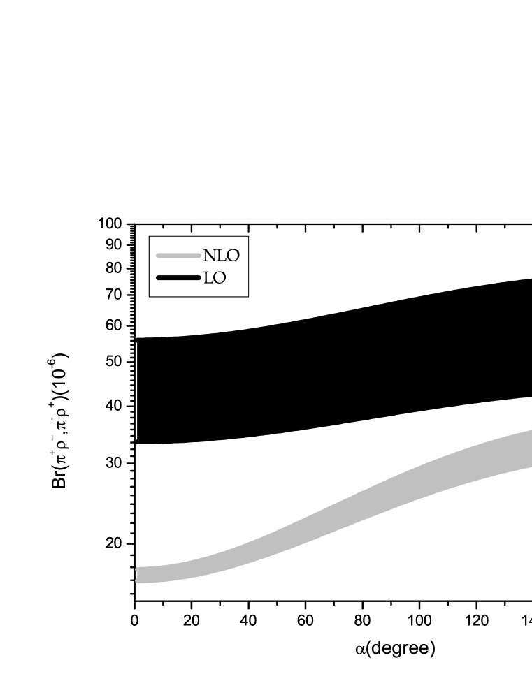
Figure 2: The scale dependence of $Br(B^{0}/\bar{B}^{0}\rightarrow\pi^{\pm}\rho^{\mp})$ of the LO(the black band) and the NLO(the gray band).

IV.2 CP asymmetries

Using (38) and (39), we can derive the direct CP-violating parameter

$$A^{dir}_{CP}=\frac{\mathcal{|\overline{A}}|^{2}-|\mathcal{A}|^{2}}{|\mathcal{A}|^{2}+\mathcal{|\overline{A}}|^{2}}=\frac{2z\sin\alpha\sin\delta}{1+2z\cos\alpha\cos\delta+z^{2}}.$$ (41)

It is clear that the non-zero direct CP asymmetry requires at least two comparable contributions with different strong phase and different weak phase. Since $A^{dir}_{CP}$ is proportional to $\sin\alpha$, it can be used to measure the CKM angle $\alpha$, if we know the strong phase difference between the tree and penguin diagrams. The CKM angle $\alpha$ dependence of the direct CP-violating asymmetries of these decays are shown in Fig. 3. The accuracy of this measurement requires more precise theoretical calculation and more experimental data.

The numerical results for the direct CP-violating asymmetries of $B^{\pm}\rightarrow\pi^{\pm}\rho^{0}$, $\rho^{\pm}\pi^{0}$, $\pi^{\pm}\omega$ and $B^{0}\rightarrow\pi^{0}\rho^{0}$, $\pi^{0}\omega$ decays are listed in Table 2. The direct CP-violation parameters of $B^{+}\rightarrow\pi^{+}\rho^{0}$ is negative, while the direct CP-violation parameter of the other modes are positive. The direct CP-violation parameter of $B^{+}\rightarrow\pi^{+}\omega$ is rather small for the almost canceled contributions of annihilation diagram, which are the dominant contributions to the strong phases in pQCD approach. Because the NLO Wilson evolution increases the penguin amplitudes and dilutes the tree amplitudes, the NLO direct CP-violation parameters (absolute value) of those decays are slightly enhanced compared with the LO predictions. However, for the color-suppressed tree dominant modes $B^{0}\rightarrow\pi^{0}\rho^{0}$ and $B^{0}\rightarrow\pi^{0}\omega$, the direct CP asymmetry varies from $-50\%$ to $47\%$ and from $52\%$ to $98\%$, respectively. The big changes are attributed to a huge change of the strong phase of color-suppressed tree amplitudes caused by the vertex corrections.

Table 2: The pQCD predictions for the direct CP-violating asymmetries of $B^{\pm}\rightarrow\pi^{\pm}\rho^{0},\rho^{\pm}\pi^{0},\pi^{\pm}\omega$ and $B^{0}\rightarrow\pi^{0}\rho^{0},\pi^{0}\omega$ decays$(\text{in units of }\%)$. We cite theoretical results evaluated in QCDF-I npb675333 , QCDF-II09095229 , SCET 0801 and experimental data pdg2010 for comparison.

Mode	LO	NLO	QCDF-I npb675333	QCDF-II 09095229	SCET 0801	Data pdg2010
$B^{\pm}\rightarrow\pi^{\pm}\rho^{0}$	-26.4	$-13.2^{+4.8+0.7+6.5+8.5}_{-5.3-0.7-5.5-9.6}$	$4.1^{+1.3+2.2+0.6+19.0}_{-0.9-2.0-0.7-18.8}$	$-9.8^{+3.4+11.4}_{-2.6-10.2}$	$-19.2^{+15.5+1.7}_{-13.4-1.9}$	$18^{+9}_{-17}$
$B^{\pm}\rightarrow\rho^{\pm}\pi^{0}$	20.1	$34.7^{+4.4+1.6+4.4+8.8}_{-4.1-1.6-4.8-8.2}$	$-4.0^{+1.2+1.8+0.4+17.5}_{-1.2-2.2-0.4-17.7}$	$9.7^{+2.1+8.0}_{-3.1-10.3}$	$12.3^{+9.4+0.9}_{-10.0-1.1}$	$2\pm 11$
$B^{\pm}\rightarrow\pi^{\pm}\omega$	0.4	$5.3^{+0.3+0.3+1.2+0.8}_{-0.1-0.3-0.5-2.5}$	$-1.8^{+0.5+2.7+0.8+2.1}_{-0.5-3.3-0.7-2.2}$	$-13.2^{+3.2+12.0}_{-2.1-10.7}$	$2.3^{+13.4+0.2}_{-13.2-0.4}$	$-4\pm 6$
$B^{0}\rightarrow\pi^{0}\rho^{0}$	-49.8	$46.5_{-8.2-2.1-2.6-7.0}^{+8.4+2.2+6.2+7.1}$	$-15.7^{+4.8+12.3+11.0+19.8}_{-4.7-14.0-12.9-25.8}$	$11.0^{+5.0+23.5}_{-5.7-28.8}$	$-3.5^{+21.4+0.3}_{-20.3-0.3}$	$-30\pm 40$
$B^{0}\rightarrow\pi^{0}\omega$	51.9	$97.6_{-1.1-2.1-1.3-3.0}^{+0.0+1.5+0.7+3.0}$	–	$-17.0^{+55.4+98.6}_{-22.8-82.3}$	$39.5^{+79.1+3.4}_{-185.5-3.1}$	–

The theoretical uncertainties of the NLO-pQCD predictions are also shown in Table 2. The first error shown in the table, comes from the B meson wave function parameters $\omega_{b}=0.40\pm 0.04$ and $f_{B}=0.21\pm 0.01\text{GeV}$; The second error arises from the uncertainties of the CKM matrix elements $|V_{ub}|=(3.47^{+0.16}_{-0.12})\times 10^{-3}$, $|V_{td}|=(9.62^{+0.26}_{-0.2})\times 10^{-3}$ and the CKM angles $\alpha=(90\pm 5)^{\circ}$; the third error comes from the uncertainties of final state meson wave function parameters $a_{2}^{\pi}=0.44^{+0.1}_{-0.2}$, $a_{\rho}^{\parallel}=0.18\pm 0.1$; the fourth error is from the hard scale $t$ varying from $0.75t$ to $1.25t$ and $\Lambda^{(5)}_{QCD}=0.228^{+0.008}_{-0.009}\text{GeV}$, characterizing the uncertainty of higher order contributions. Unlike the CP-averaged branching ratios, the direct CP asymmetry is not sensitive to the wave function parameters and CKM factors, since these parameter dependence canceled out in Eq.(41). In addition, the CKM angles ($\alpha$) uncertainty is quite small ($\sim 5\%$). Therefore, the most important uncertainties here are the scale dependence, which shows the importance of the NLO calculations.

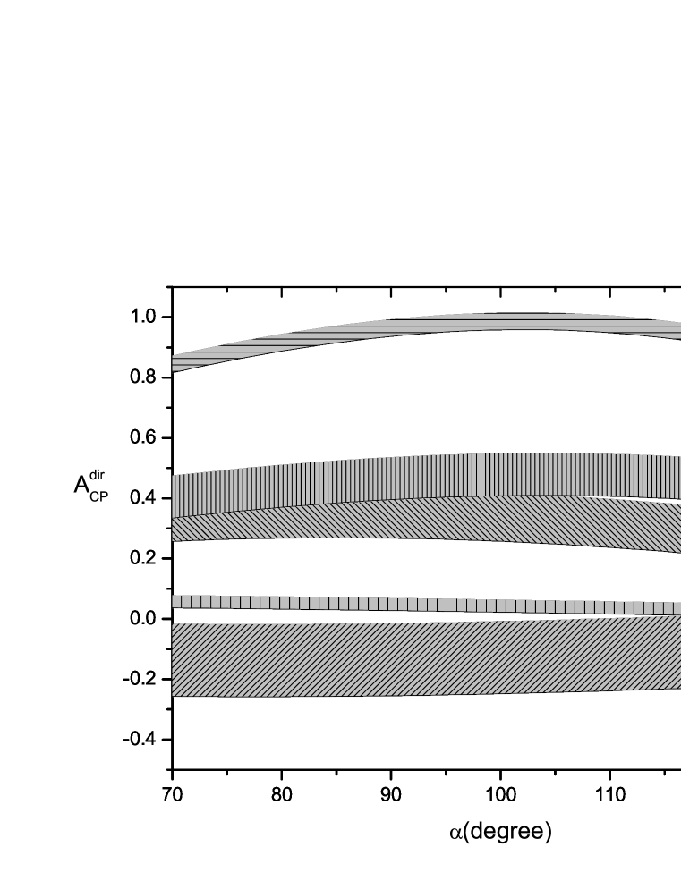
Figure 3: Direct CP-violation parameters of $B^{0}\rightarrow\pi^{0}\omega$ (the top band), $B^{+}\rightarrow\rho^{0}\pi^{0}$ (the second band), $B^{+}\rightarrow\rho^{+}\pi^{0}$ (the third band), $B^{0}\rightarrow\pi^{+}\omega$ (the fourth band), $B^{+}\rightarrow\pi^{+}\rho^{0}$ (the bottom band), as a function of CKM angle $\alpha$

.

We also cite results evaluated in QCDF-I npb675333 , QCDF-II 09095229 , SCET0801 for comparison in Table 2. Our predictions on direct CP asymmetries are typically larger in magnitude, most of which have the same sign with SCET approach. In QCDF framework, the strong phases are either at the order of $\alpha_{s}$ or power suppressed in $\Lambda_{QCD}/m_{b}$. So predictions in the QCDF-I approach on these channels are usually small in magnitude, most have different signs from our pQCD results npb675333 . In fact, the QCDF-II results 09095229 quoted in Table 2 already included large strong phase coming from penguin annihilation contributions, so that their results agree well with our pQCD ones.

For the neutral $B^{0}$ decays, the situation is more complicated due to the $B^{0}--\bar{B}^{0}$ mixing. The CP asymmetry is time dependentpdg2010 , when the final states are CP-eigenstates. A time dependent asymmetry can be defined by

$$A_{f}(t) = \frac{\Gamma(\bar{B}^{0}(t)\rightarrow f)-\Gamma(B^{0}(t)\rightarrow f)}{\Gamma(\bar{B}^{0}(t)\rightarrow f)+\Gamma(B^{0}(t)\rightarrow f)}$$ (42)

$$= S_{f}\sin\Delta mt+A_{CP}^{dir}\cos\Delta mt,$$ (43)

where $\Delta m$ is the mass difference of the two mass eigenstates of the neutral B meson. The mixing-induced CP-asymmetry parameter $S_{f}$ is referred to as

$$S_{f} = \frac{2Im(\lambda_{f})}{1+|\lambda_{f}|^{2}},$$

$$\lambda_{f} = \frac{\xi_{t}}{\xi^{*}_{t}}\frac{\mathcal{\overline{A}}}{\mathcal{A}}=e^{2i\alpha}\frac{1+ze^{i(\delta-\alpha)}}{1+ze^{i(\delta+\alpha)}}.$$ (44)

If penguin contribution is suppressed comparing with the tree contribution, we will have the approximate relation $S_{f}\simeq\sin 2\alpha$ for a negligible $z$ parameter. From Fig 4, one can see that the $S_{f}$ is not a simple $\sin 2\alpha$ behavior, since the $z\simeq 3.5$ for $\pi^{0}\rho^{0}$ and $z\simeq 1.0$ for $\pi^{0}\omega$, reflecting a very large penguin contribution.

Table 3: The pQCD predictions for the CP-violating parameters $S_{f}$ of $B^{0}\rightarrow\pi^{0}\rho^{0},\pi^{0}\omega$ (in unit of %), together with results from the QCDF-II 09095229 , the ones obtained using SCET 0801 and the experimental data pdg2010 . The errors for these entries correspond to the uncertainties in the scale dependence and other input parameters, respectively.

. Mode LO NLO QCDF-II 09095229 SCET 0801 Data pdg2010 $S_{\pi^{0}\rho^{0}}$ 47 $24^{+26+9}_{-19-12}$ $-24^{+15+20}_{-14-22}$ $-19^{+14+10}_{-14-15}$ $10\pm 40$ $S_{\pi^{0}\omega}$ -37 $21_{-10-11}^{+5+13}$ $78^{+14+20}_{-20-139}$ $72^{+36+7}_{-154-11}$ –

Figure 4: Mixing-induced CP-violation parameters $S_{\pi^{0}\rho^{0}}$ ( the gray band), mixing CP-violation parameters $S_{\pi^{0}\omega}$ (the black band), as a function of CKM angle $\alpha$.

The pQCD numerical results for the CP-violating parameters $S_{f}$ of $B^{0}\rightarrow\pi^{0}\rho^{0},\pi^{0}\omega$ are displayed in Table 3, together with the QCDF-II 09095229 and SCET 0801 results. It can be seen that the pQCD central value for $S_{\pi^{0}\rho^{0}}$ has a different sign from the other two approaches, because of the penguin contribution is bigger than the tree contribution in our approach. Our theoretical errors for these entries shown in the table correspond to the uncertainties in the scale dependence and other input parameters, respectively. It is easy to see that the uncertainty is very large. Currently, no relevant experimental measurements for the CP-violating asymmetries of these decays are available. Our predictions for these quantities are different from those in QCDF-II and SCET. We have to wait for the experimental data to resolve these disagreements.

IV.3 Time dependent asymmetry parameters of $B^{0}(\bar{B}^{0})\to\pi^{\pm}\rho^{\mp}$ decays

Table 4: The LO-and NLO-pQCD predictions for the CP-violating parameters $C$, $S$, $\Delta C$ and $\Delta S$ of $B^{0}/\bar{B}^{0}\rightarrow\pi^{\pm}\rho^{\mp}$ $(\text{in units of }\%)$, together with results from the QCDF-I npb675333 , QCDF-II09095229 , the ones obtained using SCET 0801 and the experimental data pdg2010 . The errors for these entries correspond to the uncertainties in the scale dependence and other input parameters, respectively.

Mode	LO	NLO	QCDF-I npb675333	QCDF-II 09095229	SCET 0801	Data pdg2010
$A_{CP}$	-11	$-17^{+4+4}_{-3-4}$	$1^{+0+1+0+10}_{-0-1-0-10}$	$-11^{+0+7}_{-0-5}$	$-21^{+3+2}_{-2-3}$	$-13\pm 4$
$C$	6	$15^{+2+2}_{-2-2}$	$0^{+0+1+0+2}_{-0-1-0-2}$	$9^{+0+5}_{-0-7}$	$1^{+9+0}_{-10-0}$	$1\pm 14$
$S$	-12	$-31^{+6+16}_{-3-15}$	$13^{+60+4+2+2}_{-65-3-1-1}$	$-4^{+1+10}_{-1-9}$	$-1^{+6+8}_{-7-14}$	$1\pm 9$
$\Delta C$	17	$26_{-2-8}^{+2+5}$	$16^{+6+23+1+1}_{-7-26-2-2}$	$26^{+2+2}_{-2-2}$	$12^{+9+1}_{-10-1}$	$37\pm 8$
$\Delta S$	-7	$-7^{+0+2}_{-0-1}$	$-2^{+1+0+0+1}_{-0-1-0-1}$	$-2^{+0+3}_{-0-2}$	$43^{+5+3}_{-7-3}$	$-5\pm 10$

Both $B^{0}$ and $\bar{B}^{0}$ can decay into both the $\pi^{+}\rho^{-}$ and $\pi^{-}\rho^{+}$ final states. This is an interesting example of CP asymmetry in B decays, which is the only measured combination of four channels. $A_{f}$, $\bar{A}_{f}$, $A_{\bar{f}}$ and $\bar{A}_{\bar{f}}$ are defined as follows npb361141 :

$$A_{f} = \langle\pi^{-}\rho^{+}|H_{eff}|B^{0}\rangle,\quad A_{\bar{f}}=\langle\pi^{+}\rho^{-}|H_{eff}|B^{0}\rangle,\quad$$

$$\bar{A}_{f} = \langle\pi^{-}\rho^{+}|H_{eff}|\bar{B}^{0}\rangle,\quad\bar{A}_{\bar{f}}=\langle\pi^{+}\rho^{-}|H_{eff}|\bar{B}^{0}\rangle.$$ (45)

The system of four decay modes can define the time- and flavor-integrated charge asymmetry:

$$A_{CP}=\frac{|A_{f}|^{2}+|\bar{A}_{f}|^{2}-|A_{\bar{f}}|^{2}-|\bar{A}_{\bar{f}}|^{2}}{|A_{f}|^{2}+|\bar{A}_{f}|^{2}+|A_{\bar{f}}|^{2}+|\bar{A}_{\bar{f}}|^{2}}.$$ (46)

In the standard approximation, which neglects CP violation in the $B^{0}-\bar{B}^{0}$ mixing matrix and the width difference of the two mass eigenstates, the four time dependent widths are given by the following formulas epjc23275 :

$$\Gamma(B^{0}(t)\rightarrow\pi^{-}\rho^{+}) = e^{-\Gamma t}\frac{1}{2}(|A_{f}|^{2}+|\bar{A}_{f}|^{2})[1+C_{f}\cos\Delta mt-S_{f}\sin\Delta mt],$$

$$\Gamma(\bar{B}^{0}(t)\rightarrow\pi^{+}\rho^{-}) = e^{-\Gamma t}\frac{1}{2}(|A_{\bar{f}}|^{2}+|\bar{A}_{\bar{f}}|^{2})[1-C_{\bar{f}}\cos\Delta mt+S_{\bar{f}}\sin\Delta mt],$$

$$\Gamma(B^{0}(t)\rightarrow\pi^{+}\rho^{-}) = e^{-\Gamma t}\frac{1}{2}(|A_{\bar{f}}|^{2}+|\bar{A}_{\bar{f}}|^{2})[1+C_{\bar{f}}\cos\Delta mt-S_{\bar{f}}\sin\Delta mt],$$

$$\Gamma(\bar{B}^{0}(t)\rightarrow\pi^{-}\rho^{+}) = e^{-\Gamma t}\frac{1}{2}(|A_{f}|^{2}+|\bar{A}_{f}|^{2})[1-C_{f}\cos\Delta mt+S_{f}\sin\Delta mt],$$ (47)

where $\Delta m>0$ denotes the mass difference, and $\Gamma$ is the common total width of the B meson eigenstates. $C_{f}$ and $S_{f}$ are defined as

$$C_{f} = \frac{|A_{f}|^{2}-|\bar{A}_{f}|^{2}}{|\bar{A}_{f}|^{2}+|A_{f}|^{2}},\quad S_{f}=\frac{2Im(\lambda_{f})}{1+|\bar{A}_{f}/A_{f}|^{2}},\quad\lambda_{f}=\frac{\xi_{t}}{\xi^{*}_{t}}\frac{\bar{A}_{f}}{A_{f}},$$ (48)

For decays to the CP-conjugate final state, one replaces $f$ by $\bar{f}$ to obtain the formula for $C_{\bar{f}}$ and $S_{\bar{f}}$. Furthermore, we define $C\equiv\frac{1}{2}(C_{f}+C_{\bar{f}})$, $S\equiv\frac{1}{2}(S_{f}+S_{\bar{f}})$, $\Delta C\equiv\frac{1}{2}(C_{f}-C_{\bar{f}})$ and $\Delta S\equiv\frac{1}{2}(S_{f}-S_{\bar{f}})$. S is referred to as mixing-induced CP asymmetry and C is the direct CP asymmetry, while $\Delta C$ and $\Delta S$ are CP-even under CP transformation $\lambda_{f}\rightarrow 1/\lambda_{\bar{f}}$. If $f$ is CP eigenstate there are only two different amplitudes since $f=\bar{f}$, and $\Delta C$, $\Delta S$ vanish. The complicated formulas (IV.3) return back to the simpler one in Eq.(43).

According to (38) and (39), we can write Eq.(IV.3) as

$$A_{f} = \xi_{u}T-\xi_{t}P,\quad A_{\bar{f}}=\xi_{u}T^{\prime}-\xi_{t}P^{\prime},$$

$$\bar{A}_{f} = \xi^{*}_{u}T^{\prime}-\xi^{*}_{t}P^{\prime},\quad\bar{A}_{\bar{f}}=\xi^{*}_{u}T-\xi^{*}_{t}P,$$ (49)

where T and P denote the tree diagram amplitude and penguin diagram amplitude of $B^{0}\rightarrow\rho^{+}\pi^{-}$, respectively; while $\text{T}^{\prime}$ and $\text{P}^{\prime}$ denote the tree diagram amplitude and penguin diagram amplitude of $B^{0}\rightarrow\pi^{+}\rho^{-}$, respectively. The asymmetries $\Delta S\approx\frac{2|T||T^{\prime}|}{|T|^{2}+|T^{\prime}|^{2}}\sin\theta\cos\alpha$ are suppressed by the small penguin-to-tree ratios ($|\text{P}/\text{T}|,|\text{P}^{\prime}/\text{T}^{\prime}|\ll 1$) and the small relative phase $\theta$ between T and $\text{T}^{\prime}$ ($\theta\simeq 3.4^{\circ}$), hence they are always small in pQCD factorization. This conclusion is similar to that in QCDF npb675333 ; 09095229 , although the absolute magnitude of $\Delta S$ are much larger in pQCD than in QCDF. All the CP-violation parameters of $B^{0}/\bar{B}^{0}\rightarrow\pi^{\pm}\rho^{\mp}$ decays including the LO epjc23275 and NLO results of pQCD, QCDF-I npb675333 , QCDF-II 09095229 , SCET 0801 and the experimental data are collected in Table 4. It is clear that the NLO-pQCD prediction for the CP-violation parameter $A_{CP}$, $\Delta C$ and $\Delta S$ agrees with the experimental results very well. The predictions of pQCD for CP-violation parameters in Table 4 are comparable with the QCDF-II, and are better than QCDF-I and SCET predictions, which is also shown in other B decay channels direct .

V conclusion

In the framework of the pQCD approach, we calculated the NLO QCD corrections to the $B\rightarrow\pi\rho$, $\pi\omega$ decays including the vertex corrections, the quark loops, the magnetic penguin, and the NLO Wilson coefficients, the Sudakov factor and RG factor. We found that the NLO corrections improved the scale dependence significantly, and had great effects on some of the decay channels. Our NLO-pQCD calculations agree well with the measured values. For example, compared with LO predictions, the NLO corrections decease (increase) the branching ratio of $B^{0}/\bar{B}^{0}\rightarrow\pi^{\pm}\rho^{\mp}(B^{0}\rightarrow\pi^{0}\rho^{0})$, and improve the consistency of the pQCD predictions. The NLO corrections play an important role in modifying direct CP asymmetries. For the color-allowed tree dominant modes, the NLO Wilson coefficients enhance the penguin amplitudes, the larger subdominant penguin amplitudes increase the magnitudes of the direct CP asymmetries due to the stronger interference with the dominant tree amplitudes. The predictions of pQCD for CP-violation parameters are better than QCDF-I and SCET predictions.

Appendix

We show here the hard function $h_{ql}$ and $h_{mg}$ the Sudakov exponents $S_{ql,mg}(t)$ appearing in the expressions of the decay amplitudes in III,

$$h_{ql}(x_{1},x_{2},b_{1},b_{2}) = K_{0}(\sqrt{x_{1}x_{2}}m_{B}b_{1})$$ (50)

$$\times[\theta(b_{1}-b_{2})K_{0}(\sqrt{x_{2}}m_{B}b_{1})I_{0}(\sqrt{x_{2}}m_{B}b_{2})$$

$$+\theta(b_{2}-b_{1})K_{0}(\sqrt{x_{2}}m_{B}b_{2})I_{0}(\sqrt{x_{2}}m_{B}b_{1})]S_{t}(x_{2}),$$

$$h_{mg}(A,B,C,b_{1},b_{2},b_{3}) = -K_{0}(Bb_{1})K_{0}(Cb_{3})\times\int_{0}^{\pi/2}d\theta\tan\theta$$ (51)

$$J_{0}(Ab_{1}\tan\theta)J_{0}(Ab_{2}\tan\theta)J_{0}(Ab_{3}\tan\theta)$$

where $J_{0}$ is the Bessel function and $K_{0}$, $I_{0}$ are modified Bessel functions with $K_{0}(-ix)=-(\pi/2)Y_{0}(x)+i(\pi/2)J_{0}(x)$.

The Sudakov exponents used in the text are defined by

$$S_{ql}(t)=s(x_{1}m_{B},b_{1})+s(x_{2}m_{B},b_{2})+s((1-x_{2})m_{B},b_{2})+\frac{5}{3}g_{2}(t,b_{1})+2g_{2}(t,b_{2}),$$ (52)

$$S_{mg}(t) = s(x_{1}m_{B},b_{1})+s(x_{2}m_{B},b_{2})+s((1-x_{2})m_{B},b_{2})+s(x_{3}m_{B},b_{3})$$ (53)

$$+s((1-x_{3})m_{B},b_{3})+\frac{5}{3}g_{2}(t,b_{1})+2g_{2}(t,b_{2})+2g_{2}(t,b_{3})$$

where the functions $s(P,b)$ have been defined in Ref.prd527 . The RG factor $g_{2}(t,b)$ is given by

$$g_{2}(t,b) = -\frac{2}{\beta_{0}}\ln[\frac{\ln(t/\Lambda_{QCD})}{-\ln(b\Lambda_{QCD})}]+\frac{2\beta_{1}}{\beta^{3}_{0}}[\frac{\ln(\ln(\frac{1}{b^{2}\Lambda^{2}_{QCD}}))}{\ln(\frac{1}{b^{2}\Lambda^{2}_{QCD}})}-\frac{\ln(\ln(\frac{t^{2}}{\Lambda^{2}_{QCD}}))}{\ln(\frac{t^{2}}{\Lambda^{2}_{QCD}})}$$

$$+\frac{1}{\ln(\frac{1}{b^{2}\Lambda^{2}_{QCD}})}-\frac{1}{\ln(\frac{t^{2}}{\Lambda^{2}_{QCD}})}]$$

$$\beta_{0} = 11-\frac{2}{3}n_{f},\quad\beta_{1}=102-\frac{38}{3}n_{f}$$ (54)

where $n_{f}$ is the number of quarks with mass less than the energy scale $t$.

References

• (1) I.I.Bigi, A.I.Sanda, CP violation, Cambridge.
• (2) P.Β Ball et al., CERN Yellow Report 2000-004; hep-ph/0003238.
• (3) Mario Antonelli et al. Phys. Rept. 494 (2010) 197-414.
• (4) M. Beneke, G. Buchalla, M. Neubert, and C.T. Sachrajda, Phys. Rev. Lett. 83, 1914 (1999); Nucl. Phys. B 591, 313 (2000).
• (5) C.D. LΓΌ, K. Ukai and M.Z. Yang, Phys. Rev. D 63, 074009 (2001).
• (6) Particle Data Group, J.Phys.G: Nucl.Part. Phys. 37, 075021 (2010).
• (7) S. Baek, C.-W. Chiang, D. London, Phys. Lett. B 675, 59-63 (2009) and references therein.
• (8) H.N. Li, S. Mishima, A.I. Sanda, Phys. Rev. D 72, 114005 (2005).
• (9) H.N. Li and S. Mishima, Phys. Rev. D 74, 094020 (2006); H.N. Li and S. Mishima, Phys. Rev. D 73, 114014 (2006).
• (10) Z.Q. Zhang and Z.J. Xiao, Eur. Phys. J. C 59, 49 (2009); arXiv: 0807.2024 [hep-ph].
• (11) Z.J. Xiao, Z.Q. Zhang, X. Liu, and L.B. Guo, Phys. Rev. D 78, 114001 (2008).
• (12) A. Kusaka et al., Belle Collaboration, Phys. Rev. D 77, 072001(2008); BaBar Collaboration (G Mohanty for the collaboration), talk at 5th International Workshop on the CKM Unitarity Triangle (CKM 2008), Rome, Italy, 9 C13 September 2008.
• (13) C.D. LΓΌ, M.Z. Yang, Eur. Phys. J. C 23, 275 (2002).
• (14) G. Buchalla, A.J. Buras, M.E. Lautenbacher, Rev. Mod. Phys. 68, 1125 (1996).
• (15) C.W.Bauer, S. Fleming, D. Pirjol and I. W. Stewart, Phys. Rev. D 63, 114020 (2001); C.W.Bauer, D. Pirjol and I. W. Stewart, Phys. Rev. Lett. 87, 201806 (2001).
• (16) Yong-Yeon Keum, T. Kurimoto, H.-n. Li, C.D. LΓΌ and A.I. Sanda, Phys. Rev. D 69, 094018 (2004).
• (17) B. Melic, B. Nizic, and K. Passek, Phys. Rev. D 60, 074004 (1999).
• (18) H. Kawamura, J. Kodaira, C.F. Qiao, K. Tanaka, Phys. Lett. B 523, 111 (2001), Erratum-ibid. B 536, 344 (2002); Mod. Phys. Lett. A 18, 799 (2003).
• (19) C.D. LΓΌ, M.Z. Yang, Eur. Phys. J. C 28, 515 (2003).
• (20) V.M. Braun and I.E. Filyanov , Z. Phys. C 48, 239 (1990); P. Ball, V.M. Braun, Y. Koike, and K. Tanaka, Nucl. Phys. B 529, 323 (1998); P. Ball, J. High Energy Phys. 01, 010 (1999).
• (21) M. Bander, D. Silverman and A. Soni, Phys. Rev. Lett. 43, 242 (1979); J.M. Gerard and W.S. Hou, Phys. Rev. D 43, 2909 (1991).
• (22) S. Mishima and A.I. Sanda, Prog. Theor. Phys. 110, 549 (2003).
• (23) T. Kurimoto, H.-n. Li, A.I. Sanda, Phys.Rev. D 65 014007 (2002).
• (24) H.-n. Li, Phys. Rev. D 64, 014019 (2001); Phys. Rev. D 66, 054013 (2002); Y.-Y. Keum and A.I. Sanda, Phys. Rev. D 67, 054009 (2003).
• (25) A. Ali, G. Kramer, Y. Li, C.D. LΓΌ, Y.L. Shen, W. Wang and Y.M. Wang, Phys. Rev. D 76, 074018 (2007).
• (26) Martin Beneke and Matthias Neubert, Nucl. Phys. B 675, 333 (2003).
• (27) Hai-Yang Cheng and Chun-Khiang Chua, Phys.Rev. D 80, 114008(2009).
• (28) Wei Wang, Yu-Ming Wang, De-Shan Yang and C.D. LΓΌ, Phys. Rev. D 78, 034011 (2008).
• (29) H.-n. Li and S. Mishima, Phys. Rev. D 83, 034023 (2011).
• (30) R. Aleksan, I. Dunietz, B. Kayser, F. Le Diberder, Nucl. Phys. B 361 (1991) 141.
• (31) B.-H. Hong, C.-D. LΓΌ, Sci. China G 49, 357 (2006).
• (32) Hsiang-nan Li, Phys. Rev. D 52, 7 (1995).