Gauge theories with fermions in the two-index symmetric representation

Abstract:

We summarize our recent work on gauge theories with two flavors of fermions in the two-index symmetric representation: SU(2) gauge theory with adjoint fermions, SU(3) with sextets, and SU(4) with ten-dimensional-representation fermions. All three systems have beta functions smaller than their perturbative value, approaching a fixed point near the expected two-loop zero. In all cases the mass anomalous dimension is small, under 0.5.

For the last several years we have been studying SU($N$) gauge theories with two flavors of two-index symmetric-representation fermions. These theories have been proposed as candidate models for walking technicolor [1]. To supply the phenomenology of technicolor, the theories must be confining and chirally broken, so that they possess Goldstone bosons to be eaten by the $W$ and $Z$. To supply the phenomenology of extended technicolor, that is, to generate phenomenologically viable values for quark masses without simultaneously generating too-large flavor-changing neutral currents, requires a mass anomalous dimension $\gamma_{m}$, defined by

$$\mu\frac{dm(\mu)}{d\mu}=-\gamma_{m}(g^{2})m(\mu),$$ (1)

that is large, of order unity. Technicolor models that produce both electroweak symmetry breaking and fermion mass generation are called “walking technicolor.” The coupling is presumed to run to a large value, at which $\gamma_{m}$ is large, and then to stall for many decades due to a near-zero value of the beta function, till finally chiral symmetry breaking sets in. Since the beta function and $\gamma_{m}$ are the important ingredients in the phenomenology, our work has focused on measuring them. We do this using Schrödinger-functional background-field techniques.

The status of this project is as follows:

• We observed an infrared-attractive fixed point (IRFP) in SU(2) with two flavors of adjoint-representation fermions, and we have measured $\gamma_{m}$. This is published [2].

• Last year [3] we published a result for a beta function for SU(3) with two flavors of sextet fermions, which became small in strong coupling. We could not push to stronger coupling because of the presence of a phase transition that is a lattice artifact. With new techniques (to be described below) the beta function is consistent with zero at the strongest coupling we reach.

• We are also simulating SU(4) gauge theory with two flavors of ten-dimensional fermions. Its beta function also falls from its one-loop perturbative value to zero at our strongest couplings.

In all cases the mass anomalous dimension $\gamma_{m}(g^{2})$ is small, less than 0.5 over the observed range. The data we presented at the conference have been updated to the time this report is being written. The SU(3) and SU(4) analyses, however, are still incomplete.

In the Schrödinger functional, the running coupling is defined by the response of the effective action to the boundary conditions. The scale $L$ is given by the size of the simulation volume and a scale change $s$ is achieved by performing simulations at several values ($L$, $sL$) of the volume at fixed bare couplings. Theories with many fermion degrees of freedom are characterized by slow running of the effective coupling constant. This can be seen even at one loop:

$$b(1/g^{2})\equiv\frac{d(1/g^{2})}{d\log L}=2\frac{\beta(g^{2})}{g^{4}}=2\frac{b_{1}}{16\pi^{2}}+\dots$$ (2)

where $b_{1}=-\frac{11}{3}N_{c}+\frac{4}{3}N_{f}T(R)$. The coupling then runs as

$$\frac{1}{g^{2}(s)}=\frac{2b_{1}}{16\pi^{2}}\log s+\dots$$ (3)

Now the range of scales $s$ accessible to a set of lattice simulations at any value of the bare parameters is small, certainly $s<10$. If $b_{1}$ is small, than over this range of scales the one-loop coupling will scarcely change; the system will behave as if it is nearly conformal. This behavior is expected at weak coupling, near the Gaussian fixed point. At stronger coupling, the beta function can decrease in absolute value, in which case the theory is even more nearly conformal; or it could increase, as in ordinary low-$N_{f}$ QCD. In all the cases we have studied, the beta function decreases toward zero as we move to stronger coupling.

This slow running has both good and bad consequences for a simulation. A good consequence is that the data become easy to analyze. For example, correlation functions in a near-conformal theory become pure power laws,

$$\Gamma(sp)=s^{d_{n}}\Gamma(p)\exp\int_{1}^{s}\frac{dt}{t}\gamma(g(t))\simeq s^{d_{n}}\Gamma(p)s^{\gamma(g(s))}.$$ (4)

A negative consequence is that if we want a system to be strongly interacting at long distance, it must also be strongly interacting at short distance. This means that one’s simulation can be strongly affected by discretization artifacts in the lattice action.

We fight lattice artifacts by using improved actions. Nearly all our studies use clover fermions, with “fat link” gauge connections, specifically nHYP links [4, 5]. These fermions have excellent scaling properties when used in conventional QCD simulations. The good scaling behavior we observe in these studies justifies their use a posteriori.

To carry out a Schrödinger functional study of a running coupling, we must simulate at zero fermion mass. This amounts to simulating along the $\kappa_{c}(\beta)$ line in bare parameter space. Because Wilson-type fermions suffer an additive mass renormalization, we determine the fermion mass through the axial Ward identity (AWI). Systems with Wilson-type fermions and many fermion degrees of freedom (many fundamental flavors or a few flavors of higher dimensional fermions) have an annoying first-order strong-coupling phase transition. Across this transition the AWI quark mass is discontinuous, and it jumps from a positive to a negative value. Thus there is no place where the fermions are massless in strong coupling: The $\kappa_{c}$ line just comes to an end. If we are to observe an IRFP, it must lie on the part of the $\kappa_{c}$ line which is not masked by the strong coupling transition.

The transition is a lattice artifact. Different lattice actions can move it around. For SU(2) with $N_{f}=2$ adjoints, replacing the thin-link Wilson action, used by all earlier studies [6, 7, 8, 9], with nHYP clover fermions pushed the transition back and exposed the IRFP. For SU(3) and SU(4) this change of action was insufficient; the first order transition remained at relatively weak coupling.

To this point, all our simulations had been done with the plaquette gauge action. After some trial and error we discovered that if we changed the gauge action, we could push the transition back, and study stronger coupling. We did this by supplementing the original plaquette term with an additional plaquette term, constructed with the same link as is used in the fermion action—a fat link in the higher representation,

$$S_{G} = \frac{\beta}{2N}\sum{\rm Re}\,{\rm Tr}\,U_{\mu}(x)U_{\nu}(x+\hat{\mu})U_{\mu}^{\dagger}(x+\hat{\nu})U_{\nu}^{\dagger}(x)$$

$$+\frac{\beta_{f}}{2d_{f}}\sum{\rm Re}\,{\rm Tr}\,V_{\mu}(x)V_{\nu}(x+\hat{\mu})V_{\mu}^{\dagger}(x+\hat{\nu})V_{\nu}^{\dagger}(x)$$

where $U_{\mu}(x)$ is the thin link, $V_{\mu}(x)$ is the fat link, $N$ is the number of colors, and $d_{f}$ is the dimensionality of the fermion representation. In lowest order, this action is just a quadratic form in the vector potentials of the thin and fat links. Purely empirically, we found that a positive $\beta_{f}$ does the job. We did most of our tests for SU(4), where we settled on $\beta_{f}=1.0$. For SU(3) we settled on $\beta_{f}=0.5$ and used it without extensive tests.

1 SU(2)

Now we go on to our results. We took data at lattice sizes $L=6$, 8, 12, 16. In these slowly running theories, a plot of the inverse gauge coupling versus $\log L$ at fixed $(\beta,\beta_{f},\kappa)$ is essentially a straight line, whose slope is the beta function $b(1/g^{2})$ for the inverse coupling. We determine the slope $b(1/g^{2})$ from a simple linear fit, and check for potential $a/L$ discretization effects by dropping the $L=6$ point from the fit.

As usual in Schrödinger functional calculations [10, 11, 12, 9], we obtain $\gamma_{m}$ from the renormalization factor $Z_{P}$ of the pseudoscalar density. Taking advantage of the slow running as in Eq. 4, we fit $\log Z_{P}(L)=-\gamma_{m}\log L+$ constant. Dropping the $L=6$ point or doing more complicated fits allows us to search for lattice artifacts. A detailed discussion of our fitting methodology for SU(2) may be found in Ref. [2]. We illustrate our raw data with results from the SU(2) study shown in Fig. 1.

Figure 1: (a) SF inverse coupling $1/g^{2}(L)$ vs $\log L$ in the SU(2) theory. Lines are linear fits to data at fixed bare coupling. The beta function is the slope of each line. The isolated dotted line is the AF slope. (b) Pseudoscalar renormalization constant $\log Z_{p}$ vs $\log L$ for the same simulation points. $\gamma_{m}$ is minus the slope of each line.

Fig. 2 displays our results for the beta function and $\gamma_{m}(g^{2})$. Note how the mass anomalous dimension reaches a plateau at strong coupling. Even though our determination of the IRFP $g_{*}^{2}$ has large uncertainty, the weak dependence of $\gamma_{m}$ on $g^{2}$ allows for a tight determination of the anomalous dimension at the IRFP, $\gamma_{m}(g_{*}^{2})=0.31(6)$.

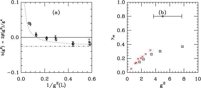
Figure 2: (a) Beta function for the inverse SF coupling in the SU(2) theory. The curves are the lowest-order and two-loop beta functions. Squares are fits to $L\geq 6$, octagons to $L\geq 8$. (b) Mass anomalous dimension $\gamma_{m}(g^{2})$ from a linear fit to the $\log Z_{p}$ vs $\log L$ data, shown as squares. The horizontal bar at the top marks our result for $g_{*}^{2}$. The crosses are the data of Bursa et al. [9], analyzed with the same linear fit.

2 SU(3)

The SU(3) gauge theory coupled to two flavors of sextet quarks has been the subject of most of our research, from a study of spectroscopy [13] to the beta function and anomalous dimension via Schrödinger functional [14] and finite-size scaling [15]. An early study with small volumes using a thin-link clover action, which indicated an IRFP [14], was superseded by a set of simulations [3] on larger volumes using fat links. The latter did show the beta function running to a small value at strong coupling, but no IRFP. The strong coupling transition prevented us from pushing further into strong coupling. With the new two-term gauge action, we can reach a coupling close to that of the two-loop Banks–Zaks [16] fixed point. At this point, we find that the beta function is consistent with zero and probably crosses zero. As in the SU(2) theory, the mass anomalous dimension follows the perturbative value out of weak coupling, until it breaks away and becomes independent of $g^{2}$, taking a value under 0.5. See Fig. 3.

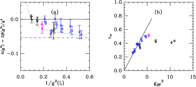
Figure 3: (a) Beta function for the inverse SF coupling in the SU(3) theory. Octagons are fits to the slopes of the lines $1/g^{2}(L)$ vs $\log L$. Diamonds drop the $L=6$ points from the fit. The curves are the lowest-order and two-loop beta functions. Blue and pink data points are from Ref. [3], obtained with $\beta_{f}=0$; the pink points were obtained in a metastable phase, past the strong coupling transition. The black points are recent data, obtained with $\beta_{f}=0.5$. (b) Mass anomalous dimension vs SF coupling, colors as in (a). The line is the one-loop result. Where they disagree, the black points supersede the blue points, which are influenced by the proximity of the lattice-artifact first-order transition.

3 SU(4)

This year we studied the third of our related theories, SU(4) gauge theory coupled to two flavors of ten-dimensional fermions. Even with nHYP links in the fermion action, the strong-coupling transition was encountered at quite a weak coupling. The fat-link gauge action, however, allows us to push farther into strong coupling. As in the case of SU(3), our strongest-coupling points are consistent with a zero beta function. (We believe that with our present actions we will be unable to push to stronger coupling because of low acceptance.) Again, the zero is at slightly weaker coupling than the Banks–Zaks point. The mass anomalous dimension again falls off the perturbative curve to take a nearly $g^{2}$-independent value, under 0.5, in strong coupling. Fig. 4 shows these results.

4 Conclusions

The analysis of the SU(3) and SU(4) systems is still in progress. Nevertheless, the outline of our conclusion is clear: Over the range where we can perform simulations the mass anomalous dimension never exceeds 0.5 in any of the three models. This strongly disfavors them as candidate theories for walking (extended) technicolor. As far as we can tell, all three models exhibit an IRFP at a value of Schrödinger functional coupling slightly weaker than expected by two-loop perturbation theory. To conclude on a positive note, these theories give theorists a set of “tame” lattice-regulated gauge theories with infrared-attractive fixed points suitable for additional studies by numerical simulation.

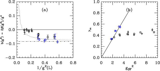
Figure 4: (a) Beta function for inverse SF coupling for $\beta_{f}=0$ and 1.0 (blue and black points, respectively), in the SU(4) theory. Plot symbols are as for SU(3). The curves are the lowest-order and two-loop beta functions. (b) Mass anomalous dimension vs SF coupling for $\beta_{f}=0$ and 1.0. The line is the one-loop result. Once again, the $\beta_{f}=1.0$ results supersede the $\beta_{f}=0$ results where they disagree.

References

- [1] For a review, see C. T. Hill, E. H. Simmons, Phys. Rept. 381, 235-402 (2003). [hep-ph/0203079].
- [2] T. DeGrand, Y. Shamir and B. Svetitsky, Phys. Rev. D 83, 074507 (2011) [arXiv:1102.2843 [hep-lat]].
- [3] T. DeGrand, Y. Shamir and B. Svetitsky, Phys. Rev. D 82, 054503 (2010) [arXiv:1006.0707 [hep-lat]].
- [4] A. Hasenfratz, F. Knechtli, Phys. Rev. D64, 034504 (2001). [hep-lat/0103029].
- [5] A. Hasenfratz, R. Hoffmann, S. Schaefer, JHEP 0705, 029 (2007). [hep-lat/0702028].
- [6] S. Catterall, F. Sannino, Phys. Rev. D76, 034504 (2007). [arXiv:0705.1664 [hep-lat]].
- [7] S. Catterall, J. Giedt, F. Sannino, J. Schneible, JHEP 0811, 009 (2008). [arXiv:0807.0792 [hep-lat]].
- [8] A. J. Hietanen, K. Rummukainen, K. Tuominen, Phys. Rev. D80, 094504 (2009). [arXiv:0904.0864 [hep-lat]].
- [9] F. Bursa, L. Del Debbio, L. Keegan, C. Pica and T. Pickup, Phys. Rev. D 81, 014505 (2010) [arXiv:0910.4535 [hep-ph]].
- [10] S. Sint and P. Weisz [ALPHA collaboration], Nucl. Phys. B 545, 529 (1999) [arXiv:hep-lat/9808013].
- [11] S. Capitani, M. Lüscher, R. Sommer and H. Wittig [ALPHA Collaboration], Nucl. Phys. B 544, 669 (1999) [arXiv:hep-lat/9810063].
- [12] M. Della Morte et al. [ALPHA Collaboration], Nucl. Phys. B 729, 117 (2005) [arXiv:hep-lat/0507035].
- [13] T. DeGrand, Y. Shamir, B. Svetitsky, Phys. Rev. D79, 034501 (2009). [arXiv:0812.1427 [hep-lat]].
- [14] Y. Shamir, B. Svetitsky, T. DeGrand, Phys. Rev. D78, 031502 (2008). [arXiv:0803.1707 [hep-lat]].
- [15] T. DeGrand, Phys. Rev. D80, 114507 (2009). [arXiv:0910.3072 [hep-lat]].
-
[16]
W. E. Caswell,
Phys. Rev. Lett. 33, 244 (1974).
T. Banks and A. Zaks, Nucl. Phys. B196, 189 (1982). - [17] http://www.physics.utah.edu/detar/milc/