Simulations of stellar convection with CO5BOLD

Abstract

High-resolution images of the solar surface show a granulation pattern of hot rising and cooler downward-sinking material – the top of the deep-reaching solar convection zone. Convection plays a role for the thermal structure of the solar interior and the dynamo acting there, for the stratification of the photosphere, where most of the visible light is emitted, as well as for the energy budget of the spectacular processes in the chromosphere and corona. Convective stellar atmospheres can be modeled by numerically solving the coupled equations of (magneto)hydrodynamics and non-local radiation transport in the presence of a gravity field. The CO5BOLD code described in this article is designed for so-called “realistic” simulations that take into account the detailed microphysics under the conditions in solar or stellar surface layers (equation-of-state and optical properties of the matter). These simulations indeed deserve the label “realistic” because they reproduce the various observables very well – with only minor differences between different implementations. The agreement with observations has improved over time and the simulations are now well-established and have been performed for a number of stars. Still, severe challenges are encountered when it comes to extending these simulations to include ideally the entire star or substellar object: the strong stratification leads to completely different conditions in the interior, the photosphere, and the corona. Simulations have to cover spatial scales from the sub-granular level to the stellar diameter and time scales from photospheric wave travel times to stellar rotation or dynamo cycle periods. Various non-equilibrium processes have to be taken into account. Last but not least, realistic simulations are based on detailed microphysics and depend on the quality of the input data, which can be the actual accuracy limiter. This article provides an overview of the physical problem and the numerical solution and the capabilities of CO5BOLD, illustrated with a number of applications.

1 Introduction

In the core of the Sun, fusion of hydrogen to helium releases energy which is transported outward, first by radiation only, but further out primarily by convection in the outer 30 % of the radial distance to the solar surface. Most of this energy is emitted in the form of radiation in the photosphere which is the bottom layer of the solar atmosphere. Furthermore, a small part of the energy is carried by waves and by magnetic fields, powering the dramatic phenomena visible in the solar chromosphere and corona. In more massive and further evolved stars, the internal structure is more complex, with several shells where nuclear burning takes place and multiple convection zones.

The relatively thin solar photosphere (about 0.1 % of the solar radius) therefore plays an important role for the inner as well as for the outer layers of the Sun. The analysis of solar and stellar spectra can reveal surface properties and the chemical composition, and allows us to draw conclusions about the internal structure and evolutionary status. For this purpose, physical models of stellar atmospheres with a realistic treatment of both radiation and convection are essential.

The classical analysis relies on one-dimensional (1D) stationary model atmospheres (in most cases only the photosphere plus the very top layers of the surface convection zone), where the average convective energy flux $F_{\rm conv}$ is computed from the so-called local mixing-length theory [1], [2], [3], a heuristic recipe which assumes that $F_{\rm conv}$ can be determined from local properties of the stratification. In the framework of this “theory”, the mean thermal structure of a convective stellar atmosphere is found by the requirement that the sum of radiative and convective flux equals the total stellar flux, $F_{\rm rad}+F_{\rm conv}=\sigma\,T_{\mathrm{eff}}^{4}$, at all depths. State-of-the-art radiative-convective equilibrium models of solar and stellar atmospheres have been constructed with the classical model atmosphere codes ATLAS [4, 5], MARCS [6, 7], and PHOENIX [8, 9], to name the most prominent examples.

A severe drawback of these models is that the efficiency of the convective energy transport is controlled by a free parameter, the mixing-length parameter $\alpha_{\rm MLT}$, which is of the order unity but a priori unknown. Therefore, $\alpha_{\rm MLT}$ must be calibrated against observations. Unfortunately, different observables require different values of $\alpha_{\rm MLT}$ [10]. The best fit of the Balmer line profiles of solar-type stars is achieved with $\alpha_{\rm MLT}\approx 0.5$ [11], while continuum colors are better reproduced with $\alpha_{\rm MLT}$ in the range 1–2, depending on the considered wavelength range [12]. The standard stellar-evolution calibration based on matching the current solar parameters calls for $\alpha_{\rm MLT}\approx 2$ [13], [14]. This disparity indicates that the underlying theoretical description is inadequate. In fact, the solar photosphere is neither homogenous nor static, since it is influenced by the very top of the convection zone and shows a granular pattern of bright upflow regions surrounded by darker intergranular lanes of downflowing material, with a spatial scale of about 1 Mm ($10^{6}$ m) and evolving on a time scale of minutes (see Fig. 1 for snapshots from two CO5BOLD simulations of the solar granulation). This motivated various efforts to overcome the limitations of the 1D classical atmospheres and to develop instead self-consistent, parameter-free hydrodynamical models of stellar surface convection, accounting for the fact that convection is a non-local, time-dependent, and intrinsically three-dimensional phenomenon.

Early idealized numerical simulations of convection under stellar-like conditions had to resort to severe simplifications (stationary 2D solutions on coarse grids) and could only deliver qualitative results: Latour et al. [15, 16] and Toomre et al. [17] used anelastic modal equations to study surface convection in A-type stars. Musman and Nelson [18] and Nelson [19] investigated convection in the Sun and some other stars with a similar method. Chan and Wolff [20] developed a code based on the alternating direction implicit (ADI) method for the calculation of compressible convection. Hurlburt et al. [21] carried out simulations of compressible solar convection extending over multiple scale heights. Steffen et al. [22] took (non-local) radiation transfer into account in their 2D simulations of compressible solar convection.

The first realistic simulations of solar granulation were performed by Nordlund [23] and included three-dimensional (3D) time-dependent hydrodynamics (but anelastic and with moderate spatial resolution) and non-local radiative energy transfer, already then with a simple treatment of the frequency-dependence of the opacities. Hand-in-hand came the a posteriori detailed spectrum synthesis by Dravins et al. [24]. Other 3D convection simulations relinquished the treatment of radiation transfer [25, 26, 27, 28, 29]. Current radiation hydrodynamic codes of various groups use similar basic techniques – in a significantly refined way (compressible hydrodynamics, more grid points, more opacity bins, larger computational domains, magnetic fields, a chemical reaction network, dust, etc.). For example, Stein and Nordlund have carried out radiation hydrodynamics (RHD) simulations with $2016\times 2016\times 500$ grid points with a spatial resolution of 24 km in the horizontal direction and 12-80 km in the vertical direction. Asplund et al. [30, 31] have computed chemical abundances using high spatial resolution and accurate radiative transfer.

Just like classical stellar atmospheres, the non-magnetic hydrodynamical models are characterized by the average total energy flux per unit area and time (effective temperature, $T_{\mathrm{eff}}$), surface gravity $g$, and chemical composition. But, in contrast to the mixing-length models, there is no longer any free parameter to adjust the efficiency of the convective energy transport. Similarly, the fudge parameters micro- and macroturbulence, that have to be introduced in 1D model atmospheres to match synthetic and observed shapes of spectral lines, are replaced by the self-consistent hydrodynamical velocity field of the 3D simulations. However, one has to keep in mind that the simulations are characterized by a large number of numerical parameters, e.g., the spatial resolution of the numerical grid, the size of the computational domain, the formulation of boundary conditions, and the parameters related to the numerical schemes for solving the hydrodynamical and radiation transport equations. Of course, the hope is that the simulation results become essentially independent of the choice of these numerical parameters, once a sufficiently high spatial, angular, and frequency resolution is achieved.

Hydrodynamical model atmospheres are not only computed for the Sun but also for other stars, and are complementing and increasingly replacing classical 1D atmosphere models. Important applications of convection simulations with CO5BOLD and its predecessor include the accurate spectroscopic determination of solar and stellar chemical abundances and isotopic ratios [e.g., 32, 33, 34], the theoretical calibration of the mixing-length parameter [35], the study of convective overshoot and mixing processes in stellar envelopes [36], and the excitation of waves by turbulent convective flows [37, 38, 39].

The presence of magnetic fields results in a wide range of additional complex 3D phenomena. Small-scale concentrations of magnetic flux lead to enhanced radiative losses, both in the photosphere and in the chromosphere. On the other hand, large-scale magnetic structures can inhibit the convective energy flux and produce the well-known dark sunspots. The interaction of convection and magnetic fields can be modeled in the framework of (ideal) magnetohydrodynamics (MHD).

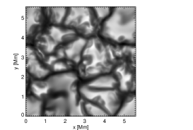
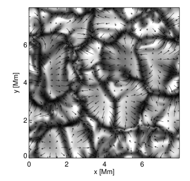
Figure 1: Emergent continuum intensity at a wavelength of $\lambda=500$ nm, synthesized for a snapshot from a high-resolution ($400\times 400\times 300$) CO5BOLD RHD simulation (left, see Sect. 4.1) and for a ($286\times 286\times 266$) CO5BOLD RMHD model (right, cf. Fig. 14), each representing a small patch of solar surface granulation. The imposed average magnetic flux of the RMHD model is $\langle B_{z}\rangle=50$ G. The arrows represent streamlines that follow the horizontal velocity on the surface of optical depth unity, i.e., at the bottom of the solar photosphere.

In the purely hydrodynamical simulations described above, the resulting mean flow is determined only by the prescribed physical quantities $T_{\mathrm{eff}}$, $g$, and the assumed chemical composition, and is largely independent of the formulation of the boundary conditions and details of the initial configuration. This is no longer true for the more complex simulations of solar magnetoconvection. In this case, the presence of a magnetic field implies more freedom in setting up the problem: the initial configuration of the magnetic field and the magnetic boundary conditions have to be designed for the particular problem under consideration. In many studies, the magnetic field is assumed to be vertical at the upper and lower boundaries, such that the horizontally averaged magnetic flux is fixed at a prescribed value. For example, $\langle B_{z}\rangle=50$ G for the CO5BOLD MHD simulation shown in Fig. 1, which is representative of the least magnetic solar-surface areas, the so-called quiet-Sun internetwork regions. The velocity arrows in this figure show that the flow converges towards the dark intergranular lanes, where cool gas returns into the solar convection zone. This flow also leads to a concentration of magnetic flux in the downflow lanes, where is is visible as bright knots or elongated features (e.g., near $x=5.5$ Mm, $y=1.5$ Mm in Fig. 1, right panel).

Early 2D MHD simulations of solar convection, which include radiative transfer were presented by Grossmann-Doerth et al. [40] based on a adaptive moving finite element code, by Steiner et al. [41] with a finite-volume code based on automatic adaptive mesh refinement for MHD, described in Steiner et al. [42], and by Atroshchenko and Sheminova [43] who used a method of approximate Eddington factors for the radiative transfer.

To our knowledge, the first realistic three-dimensional radiation magnetohydrodynamic (RMHD) simulation of stellar magnetoconvection was presented by Nordlund [44]. Nordlund et al. [45] give a review on solar surface convection including results on magnetoconvection. Early two-dimensional MHD simulations of stellar magneto-convection, which dispense with detailed radiative transfer include Galloway and Weiss [46], Deinzer et al. [47], Hurlburt and Toomre (1988) [48], Weiss et. al. (1990) [49], and Fox et al. (1991) [50].

The pioneering work of Nordlund and collaborators was only recently followed up by others, also working in three spatial dimensions. Examples include Hansteen and Gudiksen [51] and Gudiksen et al. [52] with the Bifrost code, Schaffenberger et al. [53] with CO5BOLD, and Vögler et al. [54] with the MURaM code, and more recently, by Heinemann et al. [55] using the Pencil code, Jacoutot et al. [56] with a code named SolarBox, developed by A. Wray, and Muthsam et al. [57] with the Antares code. Recent impressive large-scale 3D RMHD simulations include the supergranulation-size magnetoconvection simulations by Stein et al. [58], using a variant of the STAGGER code of Nordlund and Galsgaard [59], the simulations of sunspots and solar active regions described in Cheung et al. [60] and in Rempel et al. [61], both works using the MURaM code, as well as the exploratory MHD models that span the entire solar atmosphere from the upper convection zone to the lower corona by Hansteen et al. [62], [63], and Martínez-Sykora et al. [64], based on Bifrost or an extended version of the STAGGER code.

Other three-dimensional simulations of stellar magnetoconvection use approximations to the radiation transfer, like Abbett [65], Abbett and Fisher [66], and Isobe et al. [67]. Important results of solar magnetoconvection in three spatial dimensions were also obtained by simply replacing the radiation transfer with heat conduction, e.g., by Weiss et al. [68], Tobias et al. [69], Cattaneo [70], Ossendrijver et al. [71], or Cattaneo et al. [72]. For other applications, radiative exchange or heat conduction is not as critical as for convection, e.g., for the rise of buoyant magnetic flux tubes. Such simulations were carried out, e.g., by Archontis et al. [73] with the STAGGER code [59] or by Cheung et al. [74] with the Flash code.

Simulations of global stellar convective dynamos have been started by Glatzmaier [75]. More recent global MHD simulations of stellar convection include Browning et al. [76] with the ASH-code [77] and Dobler et al. [78] with the Pencil code. Ziegler [79] applied the Nirvana code to the problem of core collapse and fragmentation of a magnetized protostellar cloud.

Further MHD codes for potential application to realistic stellar convection simulations, which have been developed in an astrophysical context are the A-MAZE code, the Enzo code, the VAC code, or the Zeus code, for a non exhaustive list.

For reviews on solar magnetoconvection see Nordlund et al. [45], Nordlund and Stein [80], Carlsson [81], Steiner [82].

2 Basics

2.1 Basic considerations about convective scales

Ideally, hydrodynamical models of stellar convection should comprise the entire convection zone in a spherical shell with sufficient spatial resolution, and should cover all relevant time scales. In general, such a global approach is not feasible, however, for the reasons outlined in the following basic considerations.

2.1.1 Spatial scales

Presently, realistic models of stellar convection are restricted to a small representative volume located near the surface, including both the top layers of the convection zone and the photosphere, where most of the stellar radiation is emitted. In this context, it is important to realize that convection is driven by entropy fluctuations generated near the surface by radiative cooling. The deeper layers approach an adiabatic mean state and have little direct influence on the small-scale granular flows at the surface. For this reason, it is possible to obtain physically consistent ab initio models of stellar surface convection from local-box simulations that cover only a small fraction of the geometrical depth of the whole convection zone. Since the lower boundary is thus located right inside the convection zone where the total stellar luminosity is entirely carried by the convective flow, it is essential to employ an open lower boundary condition that impedes the flow as little as possible (details are given in Sect. 3.2.1).

As a typical example, let us consider a local-box simulation of the solar granulation measuring $L_{x}\times L_{y}=10$ Mm $\times 10$ Mm in the horizontal directions with periodic lateral boundary conditions in $x$ and $y$. In the vertical direction, open boundaries are imposed, and the extension of the box is assumed to be $L_{z}=4$ Mm, with $L_{z}^{-}\approx 3$ Mm ($\Delta\ln P\approx 7$) below and $L_{z}^{+}\approx 1$ Mm ($\Delta\ln P\approx 8$) above the optical surface, where $\Delta\ln P$ is the number of gas pressure e-foldings. A box of this size covers only $1.5$% of the total depth of the solar convection zone, but is large enough to accommodate several surface convection cells called granules (cf. Fig. 1), ensuring that the periodic boundary conditions do not have a critical influence on the resulting flow pattern. The minimum spatial resolution of the numerical grid is set by the requirement to cover one pressure scale height by at least $10$ grid cells. In the following, we assume that a typical grid comprises $N_{x}\times N_{y}\times N_{z}=250\times 250\times 200$ cells, where the horizontal cell size is constant ($\Delta x=\Delta y\approx 40$ km), while the vertical cell size increases with depth (in proportion to the local pressure scale height $H_{p}$, see below) from about $10$ km at the surface to about $50$ km near the bottom of the computational domain (for some actual examples see Table 1).

Figure 2: Reynolds number Re (left) according to Eq. (1), and Prandtl number Pr (right) computed from Eqs. (4) and (10) with $k=k_{0}=10\,\pi/H_{p}$, as function of radius in the envelope and atmosphere of the Sun, using the solar model by Christensen-Dalsgaard et al. [13]. In addition, the upper (dashed) curve in the right panel refers to the Mach number, $\mathrm{Ma}=v_{\mathrm{c}}/c_{\mathrm{s}}$. The vertical dashed line marks the bottom of the solar convection zone.

It is well known that the convective envelope of the Sun is characterized by very large flow Reynolds numbers, Re. Based on the standard solar model of Christensen-Dalsgaard et al. [13], we have evaluated this dimensionless number locally as

$$\mathrm{Re}=\frac{v_{\mathrm{c}}\,H_{p}}{\nu}\enspace,$$ (1)

where $H_{p}=-(\mathrm{d}\ln P/\mathrm{d}z)^{-1}$ is the local pressure scale height (e-folding length of the gas pressure $P$), $v_{\mathrm{c}}$ is the characteristic convective velocity according to classical mixing-length theory [1, 2], and $\nu$ is the microscopic (atomic plus radiative) kinematic viscosity, $\nu=(\eta_{a}+\eta_{r})/\rho$, with $\eta_{a}$ and $\eta_{r}$ calculated according to Spitzer [83] and Thomas [84], respectively. The depth dependence of Re in the solar envelope is displayed in the left panel of Fig. 2, showing that Re $>10^{10}$ in the entire convection zone. This implies that the flow is highly turbulent wherever convection occurs (see however [85]). The turbulent kinetic energy is dissipated into heat at the Komolgorov microscale, $\ell\approx H_{p}\,\mathrm{Re}^{-3/4}$, which varies between $0.05$ and $10$ cm from the top to the base of the solar convection zone. Clearly, the spatial resolution of the numerical simulations sketched above is insufficient by more than 6 orders of magnitude to properly resolve the complete turbulent cascade. All realistic stellar convection simulations therefore follow the so-called large-eddy approach, where only the largest flow structures, including the driving scales, are resolved, and the small-scale kinetic energy is dissipated at the grid scale, either by the numerical scheme or by a subgrid-scale model. Consequently, the effective numerical viscosity in such models is at least 8 orders of magnitude larger than in reality.

In addition to the Reynolds number, the properties of the flow are further characterized by the (dimensionless) Prandtl number,

$$\mathrm{Pr}=\frac{\nu}{\chi}\enspace,$$ (2)

the ratio of the coefficients describing the diffusion of momentum, $\nu$, and heat, $\chi$. In the stellar interior and atmosphere, heat transfer is dominated by radiation, which in the optically thick layers can be described as a diffusion process. The radiative diffusivity is given by

$$\chi=\frac{16\,\sigma\,T^{3}}{3\,\kappa\,\rho^{2}\,c_{v}}\enspace$$ (3)

($\sigma$: Stefan-Boltzmann constant, $T$: temperature, $\kappa$: radiative opacity per unit mass, $\rho$: mass density, $c_{v}$: specific heat at constant volume). Pr depends only on the thermodynamic state of the stellar gas. In the optically thin layers (photosphere), radiative heat exchange cannot be described as a diffusion process, and hence the definition of Pr via Eqs. (2) and (3) is no longer meaningful. Instead, Pr can be defined more generally as

$$\mathrm{Pr}=\frac{t_{\rm rad}}{t_{\rm vis}}\enspace,$$ (4)

the ratio of radiative time scale ($t_{\rm rad}$, see Eq. (10) below) to viscous time scale ($t_{\rm vis}^{-1}=\nu\,k^{2}$). However, the Prandtl number then becomes a function of wavenumber $k$ for optically thin conditions. In the solar convection zone and atmosphere, Pr ranges between $10^{-4}$ and $10^{-10}$ (see Fig. 2, right panel), indicating that the radiative energy diffusion is much more efficient than the viscous diffusion of momentum, in other words, the dynamical lifetime of a turbulent vortex is much longer than its thermal relaxation time.

In large-eddy simulations, diffusion is provided by an explicit artificial viscosity and/or by the numerical advection scheme, which leads to a diffusive cutoff at the scale of the grid resolution. In general, the effective viscosity depends on the grid resolution $\Delta x$, and on the wavenumber (and amplitude) of the local velocity perturbation. For small-scale structures close to the grid resolution, the coefficients characterizing the numerical diffusion of momentum, $\tilde{\nu}$, and heat, $\tilde{\chi}$, are of similar size, and hence the Prandtl number is of the order unity, $\mathrm{Pr}=\tilde{\nu}/\tilde{\chi}\approx 1$, as long as the radiative diffusivity is much smaller than the numerical one, $\chi\ll\tilde{\chi}\approx v_{\mathrm{c}}\,\Delta x$. This condition always holds in the bulk of the solar convection zone (assuming $\Delta x\approx H_{p}/10$). On the other hand, the effective artificial/numerical diffusion can be significantly smaller for well resolved smooth structures, such that $\chi>\tilde{\chi}$, and $\mathrm{Pr}\approx\tilde{\nu}/\chi<1$. This is especially true for the near-surface layers where the radiative diffusivity is high. Large-eddy simulations of solar-type surface convection can therefore achieve moderately low Prandtl numbers, in the sense that the physical radiative energy transport dominates over numerical diffusion of heat. In the bulk of the convection zone, however, the radiative diffusivity is too low, and hence numerically $\mathrm{Pr}\approx 1$ on all resolved scales.

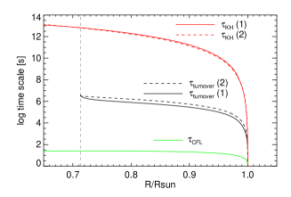
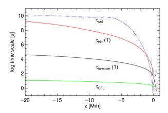
Figure 3: Left: Kelvin-Helmholtz time scale $\tau_{\rm KH}$ (upper set of curves, computed from Eqs. (5), (6)), convective turnover time scale $\tau_{\rm turnover}$ (middle set of curves, computed according to Eqs. (7), (8)), and the CFL time scale $\tau_{\rm CFL}$ (lower curve, Eq. (9)), as a function of radius in the solar envelope, based on the solar model by Christensen-Dalsgaard et al. [13]. The vertical dashed line in the left panel indicates the bottom of the solar convection zone. The right panel zooms into the upper $5$% of the convection zone, and shows in addition the radiative time scale $\tau_{\rm rad}$ calculated from Eq. (10) with $k=k_{0}=10\,\pi/H_{p}$ (dotted).

2.1.2 Time scales

The time span covered by a numerical convection simulation must be sufficiently long to ensure that the whole structure contained in the computational box can reach a thermally relaxed state. Thermal relaxation by radiative diffusion proceeds on the Kelvin-Helmholtz time scale, defined as the thermal energy content (per unit area) divided by the total energy flux: $\tau_{\rm KH}=E_{\rm th}/F_{\rm tot}$. In Fig. 3, we show the depth-dependence of $\tau_{\rm KH}$ in the solar convection zone (upper curves), computed as

$$\tau_{\rm KH}^{(1)}(r)=\frac{4\pi\,r^{2}\,\rho\,c_{p}\,T\,H_{p}}{L_{\odot}}\enspace,$$ (5)

and

$$\tau_{\rm KH}^{(2)}(r)=\frac{4\pi}{L_{\odot}}\,\int_{r}^{R_{\odot}}\,\rho\,c_{p}\,T\,r^{2}\,\mathrm{d}r\enspace,$$ (6)

respectively ($R_{\odot}$ and $L_{\odot}$ denote the solar radius and luminosity). Both expressions give essentially identical results, indicating that at a depth of $z=-3$ Mm below the solar surface, $\tau_{\rm KH}\approx 10^{6}$ s or $\approx 280$ h. Fortunately, it turns out that relaxation is significantly faster than expected from this estimate. Since the energy flux is carried by convection, a few convective turnover times are sufficient to establish a self-consistent equilibrium state. The convective turnover time scales, calculated as

$$\tau_{\rm turnover}^{(1)}(r)=\frac{H_{p}}{v_{\mathrm{c}}}\enspace,$$ (7)

and

$$\tau_{\rm turnover}^{(2)}(r)=\int_{r}^{R_{\odot}}\frac{1}{v_{\mathrm{c}}}\,\mathrm{d}r\enspace,$$ (8)

respectively, are also shown in Fig. 3 (left, middle curves). The plot shows that $\tau_{\rm turnover}\approx 2000$ s at $z=-3$ Mm, a factor $500$ smaller than $\tau_{\rm KH}$. Roughly, the simulation needs to be advanced for about 10 turnover times, $t_{\rm sim}\approx 10\,\tau_{\rm turnover}\approx 20\,000$ s to obtain a relaxed model. This number has to be related to the numerical time step $\Delta t$ applicable to the hydrodynamics scheme. The well-known Courant-Friedrichs-Lewy (CFL) condition for the stability of an explicit numerical method states that $\Delta t<\tau_{\rm CFL}$, where $\tau_{\rm CFL}$ is given by the travel time of the fastest wave across a grid cell. For the present non-magnetic example we can use the approximation

$$\tau_{\rm CFL}(r)=\frac{\Delta x}{(c_{\mathrm{s}}+v_{\mathrm{c}})}\approx\frac{H_{p}}{10\,(c_{\mathrm{s}}+v_{\mathrm{c}})}\enspace,$$ (9)

where $c_{\mathrm{s}}$ is the adiabatic sound speed. Evaluation of Eq. (9) shows that $\tau_{\rm CFL}\approx 1$ s in the upper layers (see Fig. 3).

The numerical time step is not only limited by the CFL condition. In addition, $\Delta t$ must be smaller than the characteristic radiative time scale $\tau_{\rm rad}$ that rules the decay of local temperature perturbations at the smallest possible spatial scale (wavenumber $k_{0}=10\,\pi/H_{p}$). To a good approximation, $\tau_{\rm rad}$ can be calculated as

$$\tau_{\rm rad}(r)=\frac{c_{v}}{16\,\sigma\,\kappa\,T^{3}}\,\left(1+3\,\frac{\rho^{2}\,\kappa^{2}}{k^{2}}\right)=\frac{1}{\chi}\,\left(\frac{1}{3\,\rho^{2}\,\kappa^{2}}+k^{-2}\right)\enspace,$$ (10)

which is valid in both optically thick and thin regions [86, 87]. As illustrated in Fig. 3 (right), $\tau_{\rm rad}(k_{0})$ reaches a sharp local minimum of $\approx 0.2$ s close to the optical surface. The time step of the numerical simulation is thus set by the radiative time scale, $\Delta t<0.2$ s, and the total number of required time steps is $N_{t}=t_{\rm sim}/\Delta t\approx{\color[rgb]{0,0.,0.}10^{5}}$. Assuming for reference a processor that can update $N_{c}=10^{6}$ grid cells per CPU second, the total CPU time required for this standard simulation would be $(N_{x}\times N_{y}\times N_{z}\times N_{t})/N_{c}\approx 10^{12}/10^{6}$ s or about $12$ days, which is well feasible even without a high degree of parallelization. However, it is also clear that much larger models (e.g., $10$ times better spatial resolution in each direction) are out of reach without massive parallelization.

As an example, consider the solar supergranulation which has a typical horizontal scale of 20–30 Mm. Numerical simulations of this phenomenon thus require a horizontal cross section of at least $100\times 100$ Mm². Since the spatial resolution cannot be reduced much if the granular scale still is to be resolved, such a horizontally extended simulation would take a factor $100$ more CPU time than the standard case outlined above. In addition, the simulation box would need to be extended to deeper layers for this kind of modeling. Assume that the lower boundary is moved from a depth of $z=-3$ Mm to $z=-20$ Mm, which means extending the model by about 6 more pressure scale heights. Adding $100$ grid cells in the vertical direction could be sufficient to cover the extra $17$ Mm. In terms of computing time, these extra cells are relatively cheap, because radiative transfer can be treated by the diffusion approximation in these deep layers. Note, however, that keeping the horizontal resolution at $\Delta x=\Delta y\approx 40$ km to resolve the granulation at the surface, the aspect ratio of the cells near the bottom of the box becomes rather extreme, $\Delta x/\Delta z\approx 1/10$. But the real problem is that the turnover time increases by a factor $20$. Since $\Delta t$ is set by the surface layers, the number of time steps increases by the same factor. In summary, a supergranulation simulation will take roughly a factor $2000$ more time than a standard granulation model, about $65$ years of CPU time. With massively parallel computers, such models are becoming marginally feasible (cf. [58]).

2.1.3 Global convection simulations

Simulations of the entire solar convection zone are much more expensive: the turnover time increases by another factor $100$, while the surface area is about $600$ times larger with respect to the above supergranulation model. In terms of the numbers quoted above, such a global convection simulation, which ideally should be carried out in a rotating spherical coordinate system, would take of the order of $4$ million years of CPU time, but still would cover only one year of solar time. In order to study the solar magnetic dynamo action, it would certainly be desirable to run the simulation over several $22$-year cycles, say a period 100 solar years, which is equivalent to $400$ million CPU years.

Since the surface layers set the numerical time step and spatial resolution, the computational cost can be much reduced by restricting the simulations to the deeper layers of the convection zone: here the flow Mach number is small (see Fig. 2), and the so-called anelastic approximation can be employed to avoid the time step limitation by the CFL condition; moreover, the radiative time step is very large (see Fig. 3) and does not impose any additional limitation. This approach has been adopted in the global simulations of the solar convection zone with the ASH-code by Brun et al. [88]. However, the direct link between model and observation is necessarily broken in such kind of modeling.

While realistic simulations of global solar convection remain phantasmal, prospects can be better for other type of stars: realistic global star-in-a-box simulations have already been performed successfully for red supergiants, where only a few huge convection cells occupy the surface of the star (see Sect. 4.7).

2.1.4 From the upper convection zone to the lower corona

The essential physics necessary for realistic simulations of solar surface convection includes compressible hydrodynamics describing transonic flows of a partially ionized gas in a gravitationally stratified atmosphere, coupled with non-local, frequency-dependent radiative energy exchange. In the subsurface layers, the flow becomes strongly subsonic and can be described in the anelastic approximation, while the radiative transfer becomes local and can be treated by the gray diffusion approximation. In contrast, physics becomes more complicated when considering the outer solar atmosphere.

Simulations comprising the chromosphere and lower corona must include magnetic fields. Since the magnetic field tends to form localized flux concentrations in the intergranular lanes (cf. Fig. 1, right panel), the spatial resolution of MHD simulations needs to be better than that of non-magnetic granulation models. In addition, the time step is dictated by the Alfvén speed

$$v_{\mathrm{A}}=\frac{B}{\sqrt{\mu_{0}\,\rho}}\enspace,$$ (11)

which can become much larger than the sound speed in places where the plasma-$\beta$ is low, i.e., where the magnetic field $B$ is large and the density $\rho$ is small. Typically, $\Delta t_{\rm MHD}\approx\Delta t_{\rm HD}/100$.

The low density of the outer atmosphere has also consequences for the radiation transport. Since the collision frequency is reduced, the simplifying assumption of local thermodynamic equilibrium (LTE) tends to break down, and photon scattering becomes important. This implies that the source function is no longer a function of the local temperature, but depends also on the angle-averaged radiation field. In contrast to the photospheric absorption line spectrum, the chromospheric spectrum contains strong emission lines, which dominate the energetics in the chromosphere. Under these circumstances, the solution of the radiation transfer problem becomes very time consuming.

Heat transfer by thermal conduction becomes important above gas temperatures of a few $10^{4}$ K, i.e., in the transition region and in the corona above [see, e.g., 89, 90]. Thermal conduction is usually modeled by means of the Spitzer formula but can result in a significant increase of the computational costs.

Further complications arise due to the fact that the ionization of hydrogen (and other elements) is no longer in thermal equilibrium in the low density regions, and cannot be obtained from precomputed look-up tables. Rather, the degree of hydrogen ionization, and hence the electron density, has to be derived from the solution of the time-dependent rate equations of a multi-level atom, which poses severe challenges.

For further discussion of these problems see Sect. 4.5.1, as well as Hansteen et al. [62], [63], Martínez-Sykora et al. [64], and Gudiksen et al. [52].

2.2 Equations

The hydrodynamics equations are expressed as conservation relations plus source terms for

$$\rho,\;\rho v{\rm{}_{1}},\rho v{\rm{}_{2}},\rho v{\rm{}_{3}},\;e_{\mathrm{tot}}\enspace,$$ (12)

the mass density, the three momentum densities, and the total energy density (per volume), respectively. The coordinate axes are simply numbered, in this case and in the code itself. In some sections, we use the more standard notation $x$, $y$, and $z$, though.

The three-dimensional hydrodynamics equations, including source terms due to gravity, are the mass conservation equation

$$\frac{\partial\rho}{\partial t}+\frac{\partial\;\rho\;v_{1}}{\partial x_{1}}+\frac{\partial\;\rho\;v_{2}}{\partial x_{2}}+\frac{\partial\;\rho\;v_{3}}{\partial x_{3}}=0\enspace,$$ (13)

the momentum equation

$$\frac{\partial}{\partial t}\left(\!\begin{array}[]{c}\rho v{\rm{}_{1}}\\ \rho v{\rm{}_{2}}\\ \rho v{\rm{}_{3}}\end{array}\!\right)+\frac{\partial}{\partial x_{1}}\left(\!\begin{array}[]{l}\rho v{\rm{}_{1}}\;v_{1}+P\!\\ \rho v{\rm{}_{2}}\;v_{1}\\ \rho v{\rm{}_{3}}\;v_{1}\end{array}\right)+\frac{\partial}{\partial x_{2}}\left(\!\begin{array}[]{l}\rho v{\rm{}_{1}}\;v_{2}\\ \rho v{\rm{}_{2}}\;v_{2}+P\!\!\\ \rho v{\rm{}_{3}}\;v_{2}\end{array}\right)+\frac{\partial}{\partial x_{3}}\left(\!\begin{array}[]{l}\rho v{\rm{}_{1}}\;v_{3}\\ \rho v{\rm{}_{2}}\;v_{3}\\ \rho v{\rm{}_{3}}\;v_{3}+P\!\end{array}\right)\!=\!\left(\!\begin{array}[]{c}\rho\;g{\rm{}_{1}}\\ \rho\;g{\rm{}_{2}}\\ \rho\;g{\rm{}_{3}}\end{array}\!\right)\enspace,$$ (14)

and the energy equation

$$\frac{\partial\rho e_{\mathrm{tot}}}{\partial t}+\frac{\partial\;(\rho e_{\mathrm{tot}}\!+\!P)\;v_{1}}{\partial x_{1}}+\frac{\partial\;(\rho e_{\mathrm{tot}}\!+\!P)\;v_{2}}{\partial x_{2}}+\frac{\partial\;(\rho e_{\mathrm{tot}}\!+\!P)\;v_{3}}{\partial x_{3}}{}+\frac{\partial F_{\rm 1rad}}{\partial x_{1}}+\frac{\partial F_{\rm 2rad}}{\partial x_{2}}+\frac{\partial F_{\rm 3rad}}{\partial x_{3}}=0\enspace.$$ (15)

Here $F_{\rm 1rad}$, $F_{\rm 2rad}$, $F_{\rm 3rad}$ are the components of the radiative energy flux (see below). The gas pressure $P$ is computed from the density $\rho$ and the internal energy, $e_{\mathrm{int}}$, via an equation of state, usually available to the program in tabulated form,

$$P=P(\rho,e_{\mathrm{int}})\enspace.$$ (16)

$e_{\mathrm{tot}}$ is given by the equation for the total energy,

$$\rho e_{\mathrm{tot}}=\rho e_{\mathrm{int}}+\rho\frac{v_{1}^{2}+v_{2}^{2}+v_{3}^{2}}{2}+\rho\Phi\enspace,$$ (17)

where $v_{1}$, $v_{2}$, $v_{3}$ are the components of the velocity vector, and $\Phi$ is the gravitational potential. In CO5BOLD, a prescribed, time-independent gravitational potential is used, so far. Self-gravity is not accounted for. The gravity field is given by

$$\left(\begin{array}[]{c}\rule{0.0pt}{14.22636pt}g{\rm{}_{1}}\\ \rule{0.0pt}{14.22636pt}g{\rm{}_{2}}\\ \rule{0.0pt}{14.22636pt}g{\rm{}_{3}}\\ \end{array}\right)=-\left(\begin{array}[]{c}\rule{0.0pt}{14.22636pt}\frac{\partial}{\partial x_{1}}\\ \rule{0.0pt}{14.22636pt}\frac{\partial}{\partial x_{2}}\\ \rule{0.0pt}{14.22636pt}\frac{\partial}{\partial x_{3}}\end{array}\right)\Phi\enspace.$$ (18)

With CO5BOLD, Eqs. (13)-(15) are solved with the hydrodynamics module described in Sect. 3.5.

The equations of ideal magnetohydrodynamics (MHD), including gravity and radiative energy exchange, are written in the more compact vector notation as

$$\begin{array}[]{cllll}\displaystyle\frac{\partial\rho}{\partial t}&+&\mathbf{\nabla}\cdot\left(\rho\mathbf{v}\right)&=&0\enspace,\\[8.61108pt] \displaystyle\frac{\partial\rho\mathbf{v}}{\partial t}&+&\mathbf{\nabla}\cdot\left(\rho\mathbf{vv}+\left(P+\displaystyle\frac{\mathbf{B}\cdot\mathbf{B}}{2}\right)\mathbf{I}-\mathbf{BB}\right)&=&\rho\mathbf{g}\enspace,\\[8.61108pt] \displaystyle\frac{\partial\mathbf{B}}{\partial t}&+&\mathbf{\nabla}\cdot\left(\mathbf{vB}-\mathbf{Bv}\right)&=&0\enspace,\\[8.61108pt] \displaystyle\frac{\partial\rho e_{\mathrm{tot}}}{\partial t}&+&\mathbf{\nabla}\cdot\left(\left(\rho e_{\mathrm{tot}}+P+\displaystyle\frac{\mathbf{B}\cdot\mathbf{B}}{2}\right)\mathbf{v}-\left(\mathbf{v}\cdot\mathbf{B}\right)\mathbf{B}+\mathbf{F_{\rm rad}}\right)&=&0\enspace.\end{array}$$ (19)

Here, $\mathbf{B}$ is the magnetic field vector, where we have chosen the units such that the magnetic permeability $\mu$ is equal to one. $\mathbf{I}$ is the identity matrix and $\mathbf{a}\cdot\mathbf{b}=\sum_{k}a_{k}b_{k}$ the scalar product of the two vectors $\mathbf{a}$ and $\mathbf{b}$. The dyadic tensor product of two vectors $\mathbf{a}$ and $\mathbf{b}$ is the tensor $\mathbf{ab}=\mathbf{C}$ with elements $c_{mn}=a_{m}b_{n}$ and the $n$th component of the divergence of the tensor $\mathbf{C}$ is $\left(\mathbf{\nabla}\cdot\mathbf{C}\right)_{n}=\sum_{m}\partial c_{mn}/\partial x_{m}$. In this case, the total energy is given by

$$\rho e_{\mathrm{tot}}=\rho e_{\mathrm{int}}+\rho\frac{\mathbf{v}\cdot\mathbf{v}}{2}+\frac{\mathbf{B}\cdot\mathbf{B}}{2}+\rho\Phi\enspace,$$ (20)

where $e_{\mathrm{int}}$ is again the internal energy per unit mass. The additional solenoidality constraint,

$$\mathbf{\nabla}\cdot\mathbf{B}=0\enspace,$$ (21)

must also be fulfilled. The equation of state and the equation for the gravitational field are given by Eq. (16) and Eq. (18), respectively. With CO5BOLD, the equation system, Eq. (19), is solved with the MHD module described in Sect. 3.7.

In addition, there are equations for the non-local radiation transport solved with CO5BOLD with the modules described in Sect. 3.6.3 and Sect. 3.6.4. These modules account for the frequency dependence of the opacities by the multi-group technique described in Sect. 3.6.2. In the following equations, the subscript $\nu$ refers to the index of the frequency group.

The variation of the intensity $I_{\nu}$ along a ray with direction $\mathbf{n}$ can be described by the radiative transfer equation

$$\frac{1}{\rho\kappa_{\nu}}\mathbf{n}\cdot\mathbf{\nabla}I_{\nu}+I_{\nu}=S_{\nu}\enspace.$$ (22)

The group-averaged opacities $\kappa_{\nu}$ are typically given as a function of temperature $T$ and gas pressure $P$,

$$\kappa_{\nu}=\kappa_{\nu}(T,P)\enspace,$$ (23)

and the group-integrated source function, $S_{\nu}(T)$, is normalized such that

$$\sum_{\nu}\,S_{\nu}=B(T)=\frac{\sigma}{\pi}T^{4}\enspace,$$ (24)

where $B(T)$ is the frequency-integrated Planck function. Introducing the optical depth $\tau_{\nu}$ according to

$$\rm{d}\tau_{\nu}=\rho\kappa_{\nu}\,\mathbf{n}\cdot\rm{d}\mathbf{x}\enspace,$$ (25)

where $\mathbf{n}\cdot\rm{d}\mathbf{x}$ is the path increment along the ray, the radiative transfer equation can be written as

$$\frac{{\rm d}I_{\nu}}{{\rm d}\tau_{\nu}}+I_{\nu}=S_{\nu}\enspace.$$ (26)

The frequency-integrated radiative energy flux vector in direction $\vec{n}$ is given by angular integration over the full sphere, and summation over frequency groups

$$\mathbf{F_{\rm rad}}=\sum_{\nu}\,\int_{4\pi}I_{\nu}(\Omega)\,\mathbf{n}\;{\rm d}\Omega\enspace.$$ (27)

The energy change due to radiative transfer can then be computed from the flux divergence as

$$Q_{\rm rad}=-\mathbf{\nabla}\cdot\mathbf{F_{\rm rad}}\enspace.$$ (28)

To include additional physics such as chemical reactions (Sect. 3.8.1), dynamic hydrogen ionization (Sect. 3.8.2) or dust (Sect. 3.8.3) the above equations are augmented by

$$\frac{\partial n_{i}}{\partial t}+\mathbf{\nabla}\cdot\left(n_{i}\mathbf{v}\right)=S_{i}\enspace,$$ (29)

where the number densities $n_{i}$ represent the densities of chemical species, ionization states, or dust particles. The source term $S_{i}$ accounts for chemical reactions, ionization and recombination, or dust formation.

2.3 Basic numerics

The numerical simulations described here are performed with CO5BOLD  (COnservative COde for the COmputation of COmpressible COnvection in a BOx of L Dimensions, L=2,3). It uses operator splitting [91] to separate the various (usually explicit) operators: the hydrodynamics (Sect. 3.5) or magnetohydrodynamics (Sect. 3.7), the tensor viscosity (Sect. 3.5.6), the radiation transport (different for the two setups, see below; local models: Sect. 3.6.3 or global models: Sect. 3.6.4), and optional source steps (e.g., due to time-dependent dust formation or hydrogen ionization, Sect. 3.8). The tabulated equation of state accounts for the partial ionization of hydrogen and helium and a representative metal (Sect. 3.4). The opacities can be either gray or can account for the frequency dependence via an opacity-binning scheme (Sect. 3.6.2). Parallelization is done with OpenMP.

CO5BOLD is used for two different types of model geometries, which are characterized by different gravitational potentials, boundary conditions, and modules for the radiation transport: in the local-box (or box-in-a-star) setup (Sect. 3.2.1), used to model small patches of a stellar surface, the gravitation is constant, the lateral boundaries are periodic, and the radiation transport module relies on a Feautrier scheme applied to a system of long rays (Sect. 3.6.3). In contrast, supergiant simulations employ the global or star-in-a-box setup (Sect. 3.2.2) for which the computational domain is a cube, and the grid is equidistant in all directions. All outer boundaries are open for matter and radiation. The prescribed gravitational potential is spherical. For this setup, a different radiation-transport module is used, which implements a short-characteristics method (Sect. 3.6.4).

Some more technical informations can be found in the CO5BOLD Online User Manual.

3 Detailed numerics

In this section, we present some numerical details of the code that are adapted to the conditions found in stellar atmospheres.

3.1 Numerical grid and independent variables

Instead of the conserved quantities, Eq. (12), we choose the primitive variables

$$\rho,\;v_{1},v_{2},v_{3},\;e_{\mathrm{int}}(,\;B_{1},B_{2},B_{3})$$ (30)

as independent quantities, using integer indices for the components of a vector. Since the conserved variables are purely algebraic combinations of the primitive variables, the primitive variables can be directly updated using the conservation laws Eqs. (13)-(15) or Eqs. (19) without dismissing conservation-law principles. This is explained in more details in Sects. 3.5.2 and 3.5.4.

The hydrodynamics variables $\rho,v_{1},v_{2},v_{3}$, and $e_{\mathrm{int}},$ are cell centered with grid coordinates ($x_{\mathrm{c}1},x_{\mathrm{c}2},x_{\mathrm{c}3}$), whereas $B_{1},B_{2},\mathrm{and\;}B_{3}$ are cell-boundary centered with coordinates ($x_{\mathrm{b}1},x_{\mathrm{b}2},x_{\mathrm{b}3}$). The grid is Cartesian. The grid spacing may be non-equidistant. Additional subscripts are used to describe the grid indices. The hydrodynamics variables $\rho,v_{1},v_{2},v_{3},\mathrm{and\;}e_{\mathrm{int}}$ must be thought of as cell-averaged quantities, while $B_{1},B_{2},\mathrm{and\;}B_{3}$ are mean magnetic flux densities through cell interfaces.

3.2 Boundary conditions and setup

Global models, that simulate an entire star-in-a-box (typically a red supergiant, Sect. 4.7), differ essentially in boundary conditions and the gravitational potential from local box-in-a-star models, that simulate only a small piece of a star close to the main sequence. The fundamental parameters are the effective temperature, $T_{\mathrm{eff}}$, describing the radiative flux per area in local models, or the luminosity in global models, the surface gravity, $g$, and the chemical composition of the stellar material.

3.2.1 Local models

Local box-in-a-star models are designed to simulate a small patch at the surface of a star, ignoring effects of the spherical geometry and variations in gravity. The computational domain is a Cartesian box with constant, downwardly directed gravitational acceleration given by

$$\mathbf{g}=\left(0,0,-g\right)\enspace.$$ (31)

The side boundaries are usually periodic. Closed walls are a rarely used option, as they tend to attract downdrafts.

The top boundary is generally either hit under some finite angle by an outgoing shock wave or it lets material fall back into the computational domain (often with supersonic velocities): there is not much point in tuning the formulation for an optimum transmission of small-amplitude waves [92]. Instead, a simple and stable prescription that lets the shocks pass is sufficient. It is implemented by assigning typically two or more layers of ghost cells (the number depending on the order of the reconstruction scheme), with boundary values, for which the velocity components and the internal energy are kept constant. The density is assumed to decrease exponentially with height in the ghost layers, with a scale height set to a controllable fraction of the local hydrostatic pressure scale height. The layers of ghost cells are located outside the computational domain proper. The control parameter allows for the adjustment of the mean mass flux through the open top boundary.

The bottom boundary of a standard solar model is located well inside the convection zone, where the material coming from below is assumed to have the entropy of the adiabat of the deeper convective envelope [35]. The corresponding boundary condition prescribes the entropy of the ascending material, ensures a zero total mass flux, and reduces pressure fluctuations for stability reasons. Horizontal velocities are assumed to be constant with depth. The values of $\rho$, $e_{\mathrm{int}}$, and the vertical velocity $v_{3}$ in the lowermost grid layer are actually modified during the application of this boundary condition. Therefore, the conservation laws are only valid in the volume above the bottom layer. For each cell in the bottom layer the following steps are performed:

The equation of state is solved,

$${\rm EOS}(\rho,e_{\mathrm{int}})\;\;\rightarrow\;\;s,\;P,\;T,\;\Gamma_{1},\;\Gamma_{3},\;c_{\mathrm{s}}\enspace,$$ (32)

to get the entropy, pressure, temperature, first and third adiabatic coefficient, and the sound speed. Horizontal averages of the density and pressure $\langle\rho\rangle^{(0)},\enspace\langle P\rangle$ over the entire bottom layer are computed, where the superscripts ${}^{(0)},\ldots,^{(3)}$ here and in the following equations denote the sub step. A characteristic time scale is estimated by

$$\langle t_{\rm char}\rangle=\Delta x{\rm{}_{3}}/\langle c_{\mathrm{s}}+\left|v_{3}\right|\rangle\enspace.$$ (33)

In cells with an upflow ($v_{3}>0$), mass and energy are modified according to

$$\rho^{(1)}=\rho+\mbox{C${}_{s{\rm Change}}$}\frac{\mbox{\small$\Delta$}t}{t_{\rm char}}\frac{-\rho^{2}\;T\,\left(\Gamma_{3}-1\right)}{P\;\Gamma_{1}}\,\left(s_{\rm inflow}-s\right)\enspace,$$ (34)

$$e_{\mathrm{int}}^{(1)}=e_{\mathrm{int}}+\mbox{C${}_{s{\rm Change}}$}\frac{\mbox{\small$\Delta$}t}{t_{\rm char}}T\left(\!1-\frac{\Gamma_{3}-1}{\Gamma_{1}}\right)\left(s_{\rm inflow}-s\right)$$ (35)

with the two external parameters C_sChange ($\sim$0.1) and $s_{\rm inflow}$. The latter controls the effective temperature $T_{\mathrm{eff}}$. To reduce deviations of the pressure from the horizontal mean, the following corrections are applied to all cells in the bottom layer:

$$\rho^{(2)}=\rho^{(1)}+\mbox{C${}_{P{\rm Change}}$}\frac{\mbox{\small$\Delta$}t}{t_{\rm char}}\frac{1}{c_{\mathrm{s}}^{2}}\,\left(\langle P\rangle-P\right)\enspace,$$ (36)

$$e_{\mathrm{int}}^{(2)}=e_{\mathrm{int}}^{(1)}+\mbox{C${}_{P{\rm Change}}$}\frac{\mbox{\small$\Delta$}t}{t_{\rm char}}\frac{1}{\Gamma_{1}\;\rho}\left(\langle P\rangle-P\right)\enspace,$$ (37)

adding another parameter C_PChange ($\sim$0.3). To keep the total mass in the model volume unaltered, the density in the bottom layer is corrected with

$$\rho^{(3)}=\rho^{(2)}+\langle\rho\rangle^{(0)}-\langle\rho^{(2)}\rangle\enspace.$$ (38)

Because of this step, this boundary condition acts as a closed boundary for plane-parallel waves. Finally, the vertical velocity is modified to ensure a zero-average vertical mass flux,

$$v_{3}^{(1)}=v_{3}-\frac{\langle\rho^{(3)}\,v_{3}\rangle}{\langle\rho\rangle^{(0)}}\enspace.$$ (39)

Now, the old values are replaced by the new ones,

$$\rho^{\rm(new)}=\rho^{(3)}\enspace,\enspace e_{\mathrm{int}}^{\rm(new)}=e_{\mathrm{int}}^{(2)}\enspace,\enspace v_{3}^{\rm(new)}=v_{3}^{(1)}\enspace.$$ (40)

Later, during the hydrodynamics step, the ghost cells are simply filled with constantly extrapolated values from the bottom layer while keeping the gravitational potential constant in these layers.

3.2.2 Global models

For global models, the gravitational potential depends on the radius $r$ only. The $1/r$ potential is a good approximation for the outer layers of supergiant stars, which have a small massive core surrounded by an extended low-density envelope. To avoid the central singularity the potential is smoothed near the center. The potential can also be flattened at large distances to artificially enlarge the pressure (and density) scale height preventing extremely low pressures and densities in the corners of the simulation box. The potential is given by

$$\Phi\left(r\right)=-{G\,M_{\ast}}{\left(r_{0}^{4}+r^{4}/\sqrt{1+(r/r_{1})^{8}}\,\right)^{-1/4}}\enspace,$$ (41)

where $M_{\ast}$ is the mass of the star to be modeled and $r_{0}$ and $r_{1}$ are smoothing parameters in the core and the outer envelope, respectively. Within the sphere $r<r_{0}$, a source term to the internal energy provides the stellar luminosity. Motions in the core are damped by a drag force to suppress dipolar oscillations.

All six surfaces of the computational box employ the same open boundary condition, which is also used for the top boundary in the local models (Sect. 3.2.1).

For global models the temperature/pressure range of the photospheric opacity tables is insufficient. It is therefore merged at around 12 000 K from high-temperature OPAL data [93] and low-temperature PHOENIX data [94].

3.3 Initial conditions

Due to the chaotic nature of stellar convection [95] and the primary interest in averaged or statistical properties, the details of the initial conditions hardly matter, except for initial strong magnetic field configurations. On the other hand, the total mass within the computational domain is of main importance. However, choosing a pressure and temperature distribution too far off from the (usually close to hydrostatic) mean conditions requires an unnecessarily long time, until plane-parallel pulsations have settled down and the stratification is thermally relaxed. It is often advisable to start with a standard 1D atmosphere model (e.g., produced with PHOENIX as in [96]), to expand it trivially into the second and third dimension and to add small velocity fluctuations to it as seed for convective motions. An even better alternative is to use an existing 3D snapshot with similar parameters – if available – and scale it to the desired model properties.

Even with a careful construction of the start model, transient plane-parallel pulsations are common. These pulsations are generated by tiny deviations from the exact numerical hydrostatic equilibrium in the deeper layers, causing larger amplitudes in the tenuous top layers. To damp them out, a vertical drag force acting only on the horizontal average of the vertical mass flux can be applied in the initial phase of a simulation.

3.4 Equation of state

Under the conditions of cool stellar surfaces, a lot of energy can go into the ionization of hydrogen and helium. In CO5BOLD, the equation of state (EOS) accounts for the ionization balance of HI, HII, H₂, HeI, HeII, HeIII, and a representative metal. Pre-tabulated values as functions of density and internal energy are used ($\log\rho,\log e_{\mathrm{int}}\!\rightarrow\!\log{P},\log{T},s$). In fact, the coefficients for a bicubic interpolation of ($\log{P},\log{T},s$) are stored. Thermodynamic derivatives are computed from the corresponding derivatives of the polynomials.

3.5 Hydrodynamics

In general, a hydrodynamics scheme should

1. be consistent with the original hydrodynamics equations,

2. be stable,

3. solve the hydrodynamics equations in 3D with reasonable accuracy, i.e., be of high order whenever possible and represent discontinuities with only a few grid points,

4. be conservative to handle shocks properly and give constant total fluxes in stationary cases, which is particularly important for modeling convection,

5. include source terms due to gravity in a proper way to allow static solutions, so that especially the construction of an exactly hydrostatic stratification in radiative equilibrium is possible,

6. handle a general equation of state (from a table),

7. be fast, e.g., easy to vectorize, to parallelize, and to make proper use of the various CPU caches,

8. handle various geometries (in this case 1D, 2D, and 3D models),

9. be not too complex but stay fairly simple,

10. allow the coupling with additional physics (especially radiation transport).

Solvers differ in how close they get to the individual design goals. For instance, total energy conservation might get sacrificed to improve the code stability in cases of large Mach numbers. And with detailed (read, time consuming) radiation transport modules, the performance of the (usually comparably fast) hydrodynamics modules becomes unimportant.

The hydrodynamics scheme of CO5BOLD uses a finite-volume approach. By means of operator (directional) splitting [91], the 2D or 3D problem is reduced to one dimension. To compute the fluxes across each cell boundary in every 1D column in $x_{\mathrm{c}1}$ direction, an approximate 1D Riemann solver of Roe type [97] is applied, modified to account for a realistic equation of state (Sect. 3.5.5), a non-equidistant grid (Sect. 3.5.1), and the presence of source terms due to an external gravity field (Sect. 3.5.3). The partial waves are reconstructed and advected with upwind-centered fluxes. A slope limiter (MinMod, SuperBee, but usually van Leer) [98] or a reconstruction with monotonic parabolae (Colella and Woodward [99]) is applied to decrease the order of the scheme in the neighborhood of discontinuities for keeping it stable while preserving higher-order accuracy in the case of smooth flows.

The standard Roe solver has been extended in several ways to fit the particular problem of stellar surface convection as is explained in the following subsections.

3.5.1 Non-equidistant grid

The hydrodynamics scheme handles Cartesian grids only. They may be non-equidistant in any direction. Without gravitation, the location of the cell centers $x_{\mathrm{c}1}$ has not much relevance as all quantities are either integral values within a cell (for instance the mass density) or located at the cell boundaries $x_{\mathrm{b}1}$ (for instance the mass flux). In this simple case, a non-equidistant grid would only have an effect on the reconstruction equations.

With the inclusion of gravity however, the potential energy within each cell is located at $x_{\mathrm{c}1}$. This means, that the pressure should also be located there in order to allow for a correct balance of acceleration due to the pressure gradient and the gradient of the gravitational potential.

The relative position of $x_{\mathrm{c}1,\,i}$ within $x_{\mathrm{b}1,\,i}$ and $x_{\mathrm{b}1,\,i+1}$ is not set by the hydrodynamics scheme and can be chosen within reasonable limits according to the requirements, e.g., of the radiation-transport scheme.

3.5.2 Update of the mass density and the velocity

Given the update of the density in one coordinate direction for cell $i$ in conservation-law form,

$$\Delta\rho_{i}=-\frac{\mbox{\small$\Delta$}t}{\Delta x}\left(f_{\rho,\,i+1}-f_{\rho,\,i}\right)\enspace,\qquad\rho_{i}^{\mathrm{(new)}}=\rho_{i}^{\mathrm{(old)}}+\Delta\rho_{i}\enspace,$$ (42)

where $f_{\rho,\,i}$ is the mass flux in this direction between cell $i$$-$$1$ and cell $i$, the update for the momentum in the 1-direction can be reformulated in terms of the update for the velocity as follows. From the conservation-law form

$$(\rho v_{1})_{i}^{\mathrm{(new)}}=(\rho v_{1})_{i}^{\mathrm{(old)}}-\frac{\mbox{\small$\Delta$}t}{\Delta x}\left(f_{\rho v_{1},\,i+1}-f_{\rho v_{1},\,i}\right)+\mbox{\small$\Delta$}t\,S_{\rho v_{1},\,i}\enspace,$$ (43)

where $f_{\rho v_{1},\,i}$ is the 1-momentum flux in the considered direction and $S_{\rho v_{1},\,i}$ the source term for the 1-momentum, we obtain

$${v_{1}}_{i}^{\mathrm{(new)}}={v_{1}}_{i}^{\mathrm{(old)}}-\left[\frac{\mbox{\small$\Delta$}t}{\Delta x}\left(f_{\rho v_{1},\,i+1}-f_{\rho v_{1},\,i}\right)-\mbox{\small$\Delta$}t\,S_{\rho v_{1},\,i}+\Delta\rho_{i}\,{v_{1}}_{i}^{\mathrm{(old)}}\right]\frac{1}{\rho_{i}^{\mathrm{(new)}}}\enspace.$$ (44)

$\Delta\rho_{i}$ and $\rho_{i}^{\mathrm{(new)}}$ on the right hand side of Eq. (44) are known from Eq. (42). Then, the momentum $(\rho v_{1})_{i}=\rho_{i}\,{v_{1}}_{i}$ is, up to the source term, a strictly conserved quantity. The fluxes $f_{\rho}$ and $f_{\rho v_{1}}$ are defined at the cell interfaces and determined by an approximate solution of the Riemann problem as explained in Sect. 3.5 and Sect. 3.5.5. The advantage of his formulation becomes apparent when treating the gravitational potential in the derivation of the discrete equation for the internal energy. This is explained in Sect. 3.5.4.

3.5.3 Gravity

The gravitational source term in Eq. (14) and Eq. (19) destroys the hyperbolic character of the corresponding system of equations and inhibits the direct application of an (approximate) Riemann solver. On the other hand, the separation via operator splitting is not a good idea in this case, because in stratified atmospheres the pressure gradient and the gravity tend to cancel each other (nearly). Their application in sequence – and not together in a single step – would cause spurious unwanted accelerations back and forth. On the other hand, the naive combination of the Roe solver with the source terms due to gravity into a single operator by simple addition, leads to problems because the Roe solver interpretes the strong pressure gradient in a stratified atmosphere as indication of a shock wave, which is then treated as such, causing spurious – possibly large – velocity fields.

There is some freedom in the choice of the exact reconstruction of quantities inside the cells (Mellema et al. [100]), which is used to amalgamate the hydrodynamics with the gravity operator by reducing the pressure jump across a cell boundary to the deviation from hydrostatic stratification. The latter is subtracted from the actual pressure inside the cells during the computation of the amplitudes of the partial waves. The idea is, that only pressure deviations from hydrostatic equilibrium – and not just pressure gradients – should give rise to fluxes of the partial waves. In the exact hydrostatic case, the Roe solver should “see” no sound waves. This construction does not supersede the usual source terms due to gravitation.

3.5.4 Update of the internal energy

The discrete form of Eq. (15) for the total energy is given in conservation law form by

$$\left(\rho e_{\mathrm{int}}+\rho\frac{v_{1}^{2}+v_{2}^{2}+v_{3}^{2}}{2}+\rho\Phi_{\mathrm{c}}\right)_{i}^{\mathrm{(new)}}\!\!\!=\left(\rho e_{\mathrm{int}}+\rho\frac{v_{1}^{2}+v_{2}^{2}+v_{3}^{2}}{2}+\rho\Phi_{\mathrm{c}}\right)_{i}^{\mathrm{(old)}}\!\!\!-\frac{\mbox{\small$\Delta$}t}{\Delta x}\left((f_{\mathrm{e},\,i+1}+f_{\Phi,\,i+1})-(f_{\mathrm{e},\,i}+f_{\Phi,\,i})\right),$$ (45)

where $f_{\mathrm{e},\,i}$ is the 1D flux of the total energy without the potential energy from cell $i$$-$$1$ into cell $i$ provided by the Roe solver, $f_{\Phi,\,i}$ is the flux of the potential energy and $\Phi_{\mathrm{c},\,i}$ is the gravity potential in the center of the cell. Using Eq. (42) and defining the flux of the potential energy as

$$f_{\Phi,\,i}=\Phi_{\mathrm{b},\,i}\;f_{\rho,\,i}\enspace,$$ (46)

where $\Phi_{\mathrm{b},\,i}$ is the gravity potential at the interface between cell $i-1$ and cell $i$, all terms containing the gravity potential can be combined to yield

$$\left(\rho e_{\mathrm{int}}\right)_{i}^{\mathrm{(new)}} = \left(\rho e_{\mathrm{int}}\right)_{i}^{\mathrm{(old)}}+\left(\rho\frac{v_{1}^{2}+v_{2}^{2}+v_{3}^{2}}{2}\right)_{i}^{\mathrm{(old)}}-\left(\rho\frac{v_{1}^{2}+v_{2}^{2}+v_{3}^{2}}{2}\right)_{i}^{\mathrm{(new)}}-\frac{\mbox{\small$\Delta$}t}{\Delta x}\left(f_{\mathrm{e},\,i+1}-f_{\mathrm{e},\,i}\right)$$ (47)

$$-\frac{\mbox{\small$\Delta$}t}{\Delta x}\left[\left(\Phi_{\mathrm{b},\,i+1}-\Phi_{\mathrm{c},\,i}\right)f_{\rho,\,i+1}-\left(\Phi_{\mathrm{b},\,i}-\Phi_{\mathrm{c},\,i}\right)f_{\rho,\,i}\right]\enspace.$$

The presence of the new kinetic energy at the right side of Eq. (47) does not make the scheme implicit, since the velocity does not depend on $e_{\mathrm{int}}$ – it is known from Eq. (44) and corresponding equations for $v_{2}$ and $v_{3}$. We note that this update still conserves the total energy, Eq. (17), to machine accuracy. The conservative inclusion of the radiative energy flux into the energy equation is treated in Sect. 3.6.3.

3.5.5 General equation of state including ionization

Several extensions of the Roe scheme for a general equation of state have been proposed, see [101] and references therein. The differences compared to the case of an ideal gas with constant $\gamma$ manifest themselves in the need of additional Roe averages depending on which variables are used in the equation of state. For a general equation of state of the form Eq. (16), averages of $\rho$, $e_{\mathrm{int}}$ and of the pressure derivatives ${\left.\frac{\partial P}{\partial\rho}\right|_{e_{\mathrm{int}}}}$ and ${\left.\frac{\partial P}{\partial e_{\mathrm{int}}}\right|_{\rho}}$ are required to build the Roe matrix. Choosing the usual Roe average for $e_{\mathrm{int}}$ and the average $\sqrt{\rho_{l}\rho_{r}}$ for the density, where $\rho_{l}$ and $\rho_{r}$ is the density on either side of the cell interface, the condition

$$\Delta P={\left.\frac{\partial P}{\partial e_{\mathrm{int}}}\right|_{\rho}}\Delta e_{\mathrm{int}}+{\left.\frac{\partial P}{\partial\rho}\right|_{e_{\mathrm{int}}}}\Delta\rho\enspace,$$ (48)

must be fulfilled by the averages of ${\left.\frac{\partial P}{\partial\rho}\right|_{e_{\mathrm{int}}}}$ and ${\left.\frac{\partial P}{\partial e_{\mathrm{int}}}\right|_{\rho}}$ where $\Delta P$, $\Delta\rho$ and $\Delta e_{\mathrm{int}}$ are the jumps of the pressure, density, and internal energy at the cell interface. Eq. (48) is not sufficient to determine the averages of the pressure derivatives. Glaister [102] suggested formulas for ${\left.\frac{\partial P}{\partial\rho}\right|_{e_{\mathrm{int}}}}$ and ${\left.\frac{\partial P}{\partial e_{\mathrm{int}}}\right|_{\rho}}$ which meet Eq. (48) exactly. However, Glaister’s formulae do not lead to the same averaged sound speed as the original formulae of Roe in the simple case of constant $\gamma$. Furthermore, they may also produce unphysical average states [101]. In CO5BOLD, the averaging of the pressure derivatives is avoided. Instead, the dimensionless quantities $\Gamma_{1}$ and ${\left.\frac{\partial\rho e_{\mathrm{int}}}{\partial P}\right|_{s}}$ are averaged with the usual Roe weights, which ensures the consistency with the simple gas case.

The pressure derivatives in the Roe matrix lead to an additional term

$$-\frac{1}{2}|v_{1}|\left(e_{\mathrm{int}}-\rho\displaystyle{{\left.\frac{\partial P}{\partial\rho}\right|_{e_{\mathrm{int}}}}}\displaystyle{{\left.\frac{\partial P}{\partial e_{\mathrm{int}}}\right|_{\rho}}}^{-1}\right)\tilde{\alpha}^{(5)}=-\frac{1}{2}|v_{1}|\tilde{\alpha}^{(6)}\enspace,$$ (49)

in the energy flux. This term, which vanishes in the perfect gas case, is treated as a contribution from a sixth partial wave $\tilde{\alpha}^{(6)}$. The wave strength of the entropy wave $\tilde{\alpha}^{(5)}$ is given by

$$\tilde{\alpha}^{(5)}=\Delta\rho-\frac{\Delta P}{c_{\mathrm{s}}^{2}}\enspace.$$ (50)

The term ${\left.\frac{\partial P}{\partial e_{\mathrm{int}}}\right|_{\rho}}$ in Eq. (49) can become small, possibly causing numerical errors. Using thermodynamic relations, $\tilde{\alpha}^{(6)}$ can be transformed into

$$\tilde{\alpha}^{(6)}=\Delta(\rho e_{\mathrm{int}})-{\left.\frac{\partial\rho e_{\mathrm{int}}}{\partial P}\right|_{s}}\Delta P\enspace.$$ (51)

which uses a better behaved derivative.

3.5.6 Tensor viscosity

In addition to the stabilizing mechanism inherent in an upwind scheme with monotonic reconstruction, a 2D or 3D tensor viscosity can be activated. It eliminates certain errors of Godunov-type methods occurring in the case of strong velocity fields aligned with the grid [103]. Other types of problems can occur when e.g., a shock, which has a strength that could easily be handled by the hydrodynamics scheme alone, gives rise to so large opacity variations that the radiation-transport routines might get unstable (Sect. 3.6).

To overcome such (possible) problems, an additional tensor-viscosity sub step was included in the code, that can add dissipation in a way the Roe solver by its own is not able to produce. The kinematic viscosity is

$$\nu = \frac{1}{3}\left(\Delta x{\rm{}_{1}}+\Delta x{\rm{}_{2}}+\Delta x{\rm{}_{3}}\right)C_{\rm linear}\,c_{\mathrm{s}}+\min\left(\Delta x{\rm{}_{1}},\Delta x{\rm{}_{2}},\Delta x{\rm{}_{3}}\right)\max\left(\Delta x{\rm{}_{1}},\Delta x{\rm{}_{2}},\Delta x{\rm{}_{3}}\right)$$

$$\!\!\left\{\rule{0.0pt}{19.91692pt}\;C_{\rm artificial}^{2}\max(-\nabla v,0)\right.$$

$$+C_{\rm Smagorinsky}^{2}\left[\rule{0.0pt}{17.07164pt}2\left(\frac{\Delta v_{1}}{\Delta x{\rm{}_{1}}}^{2}+\frac{\Delta v_{2}}{\Delta x{\rm{}_{2}}}^{2}+\frac{\Delta v_{3}}{\Delta x{\rm{}_{3}}}^{2}\right)\right.\;\;+\left.\left.\left(\frac{\Delta v_{1}}{\Delta x{\rm{}_{2}}}+\frac{\Delta v_{2}}{\Delta x{\rm{}_{1}}}\right)^{2}+\left(\frac{\Delta v_{1}}{\Delta x{\rm{}_{3}}}+\frac{\Delta v_{3}}{\Delta x{\rm{}_{1}}}\right)^{2}+\left(\frac{\Delta v_{2}}{\Delta x{\rm{}_{3}}}+\frac{\Delta v_{3}}{\Delta x{\rm{}_{2}}}\right)^{2}\right]^{1/2}\right\}$$

with the parameters $C_{\rm linear}$, $C_{\rm artificial}$, and $C_{\rm Smagorinsky}$ for the linear, artificial (von Neumann type) viscosity, and turbulent subgrid-scale viscosity (Smagorinsky [104]), respectively. Typical values are (0, 0.5, 0.5), respectively. Models of solar granulation and similar easy cases do not require this extra viscosity. However, it is usually activated to avoid the necessity to tune the numerical parameters individually for each stellar model. For instance the models of the more dynamic atmospheres of red supergiants (Sect. 4.7) need some amount of extra dissipation provided by the tensor viscosity. Note that the tensor viscosity should not be mistaken for a hyperviscosity. The task of hyperviscosities is in CO5BOLD done by the reconstruction schemes (MinMod, SuperBee, van Leer, PP, etc.).

3.6 Radiation transport

3.6.1 Introduction

In dynamical simulations which take time dependence and coupling between radiative energy transfer and hydrodynamics equations into account, the emitted intensity is only a by-product. Important is instead the energy change per numerical grid cell due to the difference of radiative gains and losses. The requirement to solve the radiation-transport equations for many grid points and many time steps calls for severe simplifications as, e.g., the restriction to gray opacities or to a few frequency groups (Sect. 3.6.2) or the treatment of scattering as true absorption. Actually, this can make code development easier. But still, there are additional demands on the algorithm: the scheme should conserve the total energy, i.e., internal sources and sinks of energy minus losses through the surface should exactly sum up to zero. The scheme has to be stable enough to handle complex structures which may sometimes be poorly resolved (e.g., chromospheric shocks, Sect. 4.5).

Some cases pose only low demands on the complexity of the algorithm: if the entire model is optically thick, a diffusion approximation using only differences between neighbor cells is adequate to compute the radiative flux. This results in a stable scheme, if the time step is properly limited. If the whole numerical domain is optically thin and the radiation field is simple enough, a local cooling function might be sufficient to model radiative energy losses, calling for a scheme that is stable if the time step is small enough.

However, stellar atmospheres are per definition at the transition between optically thick and thin regions. The main form of energy transport switches from convective plus radiative in the interior to mainly radiative in the outer layers, where mechanical energy fluxes become very small due to the low material density. Still, mechanical energy fluxes might be sufficiently large to affect the temperature structure of the chromosphere (Sect. 4.5), for example. While radiative energy transport in the stellar interior can be properly described by local physical quantities through the diffusion approximation, in the outer layers, radiative energy exchange occurs non-locally. This means that the local radiative flux depends on the physical state of the material in the wider surroundings of a size depending on the mean free path of the photons. Large opacity variations due to changes in the ionization states of major constituents or due to shock waves can cause changes in the source function on small spatial scales. In numerical models, these two effects, amplified by fluctuations in heat capacity, can cause enormous jumps in the radiative relaxation time scale from grid point to grid point.

Even if a standard scheme is able to overcome all these difficulties and to compute accurate intensities for given opacities and source function, there are still several possibilities how to derive the induced energy change per cell, as detailed in the following:

The energy flux through the cell boundaries can be computed from the intensity field, which then gives the divergence of the flux for each cell, and hence the energy change per cell according to Eq. (28). This would guarantee the conservativity of the scheme. But unfortunately, the latter step requires an extreme numerical precision in optically very thin regions where the relative flux changes from cell to cell are tiny. A high accuracy is also necessary in optically very thick regions where only small deviations of the intensity from the local source function contribute to the net flux. Calculating a discrete derivative naturally amplifies noise and has centering problems, when e.g., the intensity field is given at cell centers and the divergence is required at the same position.

Another possibility consists in deriving the energy change per cell from the difference of the angular mean of the intensity,

$$J_{\nu}=\frac{1}{4\pi}\int_{4\pi}I_{\nu}\;\mathrm{d}\Omega={\color[rgb]{0,0.,0.}\frac{1}{4\pi}}\int_{0}^{2\pi}\int_{0}^{\pi}I_{\nu}\sin\theta\;{\rm d}\theta\;{\rm d}\varphi\enspace,$$ (53)

and the local source function $S_{\nu}$. Using Eqs. (22), (27), and (28), one obtains

$$Q_{\mathrm{rad}}=\sum_{\nu}4\pi\kappa_{\nu}\rho\;\left(J_{\nu}-S_{\nu}\right)\enspace.$$ (54)

This scheme does not have an explicit conservation form and in fact it will most likely not be conservative. This happens because the distribution of the source function within the cell which is used in the integration process for the intensity (where typically some high-order interpolation of the source function with optical depth is performed) is not exactly the same distribution as is used in computing the difference $J_{\nu}-S_{\nu}$ (where the source function is assumed to be constant). Another problem of this scheme is the accuracy in optically very thick regions, where numerical cancellation may occur between $J_{\nu}$ and $S_{\nu}$. A more indirect way is to derive from the intensity field some geometrical information about the radiation field in the form of Eddington factors. These are inserted into the equations describing the radiation transport via the Eddington moments (see, e.g., for two dimensions Stone et al. [105] and for one dimension Höfner et al. [106], [107]). This method requires a non-trivial solver to get the radiation field in the first place and later an algorithm to solve the huge system of Eddington equations. This procedure might not suffer from the problems mentioned above. However, it seems somewhat inefficient first to compute the intensity distribution of the radiation field in some detail and then to throw away most of the information and retain the Eddington factors only, which are used to solve the radiative transfer equation again – just in a different form. The extra effort can be justified by gains due to, e.g., an elegant handling of scattering processes or the achievement of large time steps with an implicit operator [106], though.

In Sect. 3.6.3 and Sect. 3.6.4, we present two radiation-transport schemes implemented in CO5BOLD, that overcome the aforementioned problems in different ways. They compute the contribution to the energy change per cell on-the-fly during the integration of the intensity for each direction. For standard local-box models with periodic boundaries (Sect. 3.2.1), we use a long-characteristics scheme, described in Sect. 3.6.3, while for star-in-a-box models with all-open boundaries (Sect. 3.2.2), we use a short-characteristics method, outlined in Sect. 3.6.4.

3.6.2 Opacity binning

The rate of the radiative energy exchange is highly variable over the relevant spectral range, since the absorption coefficient strongly varies with frequency due to the presence of spectral lines, on top of the more gradual change of the continuous opacity. In cool stars like the Sun, spectral lines count in the millions so that an exact treatment of the frequency dependence in a complex multi-dimensional geometry is beyond present computer capacities, and one has to resort to an approximate treatment. An important simplification stems from the fact that one is not interested in the detailed frequency dependence of the heat exchange between stellar plasma and radiation field but only in its frequency-integrated total effect, $Q_{\rm rad}$. Nowadays, all multi-dimensional hydrodynamical stellar atmosphere codes employ the so-called opacity-binning technique. The method was first laid out by Nordlund [23], and later refined in works by Ludwig [108], Ludwig et al. [109], and Vögler [110]. At present, opacity sampling – a statistical technique widely applied in standard 1D model atmospheres – is discussed as possible replacement of the opacity binning due to its better controlled accuracy and greater flexibility.

The basic idea of opacity binning is the classification of frequency points by the similarity of their associated $\Lambda$-operator – the operator relating source function $S_{\nu}$ and mean intensity $J_{\nu}$ of the radiation field:

$$J_{\nu}=\Lambda_{\nu}\left[S_{\nu}\right]\enspace.$$ (55)

We added an index $\nu$ to the $\Lambda$-operator to emphasize that its form, written in geometrical coordinates, is different for different frequencies due to opacity variations. However, in cases where the operator happens to be similar, its linearity allows to operate on the sum of the source functions to obtain the integrated mean intensity, symbolically expressed as

$$J_{1+2}\equiv J_{1}+J_{2}=\Lambda_{1}\left[S_{1}\right]+\Lambda_{2}\left[S_{2}\right]\approx\Lambda\left[S_{1}+S_{2}\right]\enspace,$$ (56)

where $\Lambda$ is some suitable mean of $\Lambda_{1}$ and $\Lambda_{2}$. The problem now is to classify all frequencies into distinct sets $\Omega_{i}$ grouping together as similar as possible $\Lambda$-operators. The $\Lambda$-operator can be calculated from the monochromatic optical depth scale $\tau_{\nu}$ so that the classification can be equivalently done by grouping frequencies with a similar relation between geometrical and optical depth scales. This is in fact the way how one proceeds in practice.

When trying to classify the frequencies, one is confronted with the problem that the optical depth scales depend on the atmospheric model under consideration, i.e., its geometry, the ensuing thermal conditions, and velocities. One has to choose a reference model for which the classification is performed. Naturally, this reference model is chosen to be close to the stellar atmosphere to be simulated, in the simplest case a 1D model of the atmosphere in question. Other choices are possible, but in any case, the resulting classification is optimized for a particular set of atmospheric parameters and has to be repeated when numerical simulations in other parameter regimes are conducted. Since even for fixed atmospheric parameters a large variety of different thermodynamic conditions are met along various lines-of-sight in a numerical model (with correspondingly different $\tau_{\nu}$), limits to the achievable accuracy by the opacity binning have to be expected. Thus only a reasonable similarity among $\tau_{\nu}$-scales within an opacity bin is aimed at in practice. Typically one is content if the $\tau_{\nu}$-scales of a group of frequencies share the property to reach unity within a given range of depth – usually defined via the frequency-independent Rosseland optical depth. This emphasizes the emergent radiation intensity as the primary quantity to be captured correctly, obviously an important quantity linked to the overall flux properties of a stellar atmosphere. Each opacity bin defines a corresponding frequency group.

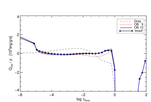
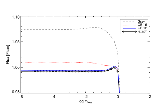
Figure 4: Performance of the opacity-binning scheme, illustrated for a 1D solar model atmosphere. The net radiative heating rate per unit mass, $Q_{\rm rad}/\rho$ (top), and the bolometric radiative flux, $F_{\rm rad}/F_{\odot}$ (bottom), and are shown as a function of Rosseland optical depth. In each panel, the results from gray (dashed), 5-bin/5-group (dotted), and 9-bin/12-group (solid) radiative transfer are compared with the “exact” solution (diamonds), obtained with very high frequency resolution.

At present, typically between four and twelve frequency groups $\Omega_{i}$ are used, depending on the desired precision. An estimate of the precision is obtained by comparing the integral radiative heating (or cooling) rates obtained from the binned opacities with the result obtained at high frequency resolution, both as a function of depth in the reference structure used for defining the opacity bins. The estimate relies on the assumption that the reference structure is indeed representative of the conditions encountered in the flow simulation. Some refinements to this basic scheme are nowadays often added. For instance, it is sometimes advantageous to split an opacity bin as defined before into frequency sub-groups, with the idea to separate frequency points which systematically heat or cool particular atmospheric layers. This helps to improve the overall energy exchange budget.

An example is given in Fig. 4, illustrating the results obtained for the 1D solar reference atmosphere. The basic 5-bin/5-group scheme is clearly superior to the gray approximation. The more sophisticated 9-bin/12-group scheme, in which three opacity bins are split into two frequency sub-groups, performs very satisfactory and almost perfectly reproduces the “exact” heating rate.

The binned opacities are obtained from a suitable average of the opacities in a particular frequency group and stored in look-up tables as a function of thermodynamic variables – in CO5BOLD as a function of gas pressure and temperature. In addition, the Planck function (as source function), integrated over the frequencies of a group, is stored as a function of temperature. This approach only works if the opacities and the source function can be calculated from the thermodynamic conditions alone, i.e., are thermodynamic equilibrium quantities. While this is often fulfilled to good approximation, there are exceptions. For instance, the formation of dust clouds in cool stellar atmospheres is a non-equilibrium process (Sect. 3.8.3), and actual particle properties are only known after solving the governing kinetic equations, taking into account the history of the evolution of a particular mass element in the flow. In CO5BOLD, we proceed by separating the equilibrium part (gas opacities) from the non-equilibrium part (dust opacities). The gas opacities are binned into frequency groups in the usual way, and the dust opacities are calculated during the simulation on-the-fly and added to the gas opacities. Obviously, this increases the computational demands.

All in all, opacity binning has been and still is working perhaps better than one might expect from the numerous approximations behind the construction of the scheme. Opacity binning has proved to be an efficient way to include the frequency dependence of the radiative transfer in multi-dimensional simulations. However, as alluded to already before, the increased computing power might allow to re-consider the approach trading greater computational costs for higher physical fidelity. The path to largest gains needs to be identified yet.

3.6.3 Long-characteristics radiation transport

The purpose of this algorithm is to compute the net radiative heating rate per unit volume, $Q_{\mathrm{rad}}(x_{i},y_{j},z_{k})$, at the center of each cell of the hydrodynamical grid (HD grid). The basic idea is to solve the equation of radiative transfer on a system of straight long rays (long-characteristics, LC) running from the upper to the lower model boundary at a number of different azimuthal angles $\phi$ and inclinations with respect to the vertical ($0\leq\theta<\pi/2)$. As a result, we obtain for each frequency group $\nu$ and for all bundles of rays with orientation $(\theta,\phi)$ the quantity $Q_{\mathrm{rad},\nu}(\theta,\phi)=\overline{\rho\kappa_{\nu}}\;\left(u_{\nu}(\theta,\phi)-S_{\nu}\right)$ at the mesh points along the rays, where the mean-intensity-like variable $u_{\nu}(\theta,\phi)$ is the average of incoming ($I_{\nu}^{-}$) and outgoing ($I_{\nu}^{+})$ intensity, $u_{\nu}=(I_{\nu}^{+}+I_{\nu}^{-})/2$ (see Fig. 5), $S_{\nu}$ is the group source function, and $\overline{\rho\kappa_{\nu}}$ is the group opacity averaged over the neighboring mesh points along the ray (see Eq. 63). $Q_{\mathrm{rad}}(x_{i},y_{j},z_{k})$ is then constructed by interpolating $Q_{\mathrm{rad},\nu}(\theta,\phi)$ from the ray system to the cell centers of the hydrodynamics grid, and appropriate angular averaging and summation over frequency groups.

Note that the technique described here basically evaluates $Q_{\mathrm{rad}}$ according to Eq. (54). It overcomes the difficulties explained in the context of Eq. (54) by solving the transport equation for the difference between mean intensity and source function, $p_{\nu}\equiv u_{\nu}-S_{\nu}$ (see Eq. 57), which gives accurate values of $(u_{\nu}-S_{\nu})$ for arbitrarily large optical depth. At the same time, it allows $Q_{\mathrm{rad},\nu}$ to be computed such that energy conservation is enforced (see Eq. 65). The procedure is very similar to that described in [23].

To simplify matters, $\phi$ is restricted to $0,(1/2)\pi,\pi,(3/2)\pi$, i.e., we consider only 2D ray systems in vertical slices along the $x$ and $y$ axis of the hydrodynamical grid. The $\theta$ angles are given by Lobatto’s quadrature formula [111]; typically, 2–4 non-zero inclination angles are sufficient, in addition to a set of vertical rays. All rays start at the cell centers of the uppermost level of the HD grid and follow the specified direction, assuming periodic lateral boundary conditions, until they reach the bottom of the computational domain.

As indicated in Fig. 5, the mesh points along the rays are defined as the intersection points with the $z$-planes of the HD grid. As this recipe would imply a rather coarse sampling along strongly inclined rays, we introduce additional horizontal planes such that the geometrical separation of mesh points along the inclined rays remains comparable to the vertical resolution of the original HD grid. The coordinates of the ray points, $(x_{mk},z_{k})$, where $m$ is the ray index and $k$ is the depth index of the refined HD grid, are equidistant in $x$.

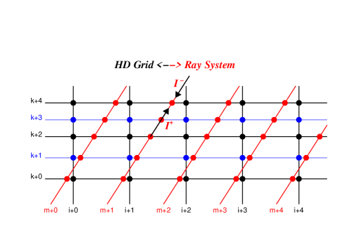
Figure 5: Schematic illustration of the different grids used with the long-characteristics radiative transfer method. The hydrodynamics equations are solved on a Cartesian grid (HD grid, black, dots representing cell centers), while the radiative transfer equation is solved on a system of inclined rays (red, dots representing the mesh points used with the Feautrier scheme). The HD grid can be refined in vertical direction by additional $z$-planes (thin, blue) to provide sufficient resolution for strongly inclined rays. The cell centers of the refined HD grid have indices ($i,k$), the mesh points along the rays have indices ($m,k$).

The main steps of the whole procedure may be summarized as follows: first, the source function, $S_{\nu}$, and the opacity per unit volume, $\rho\,\kappa_{\nu}$, are interpolated from the HD grid to the mesh points of the ray system. Linear interpolation of $S_{\nu}$ and $\log(\rho\,\kappa_{\nu})$ is adopted for the vertical direction (additional $z$-planes), while linear interpolation of $S_{\nu}$ and $\rho\,\kappa_{\nu}$ is used in horizontal direction. Note that only a 1D interpolation along the Cartesian grid lines is required. Given $\rho\,\kappa_{\nu}$ on the mesh points along the rays, we represent $\rho\,\kappa_{\nu}$ between two mesh points by a monotonic cubic polynomial [112] to obtain the optical depth increments $\Delta\tau_{\nu}$ by analytical integration. Next, we solve the equation of radiative transfer along bundles of rays in the form of the second-order differential equation:

$$\frac{{\rm d}^{2}p_{\nu}}{{\rm d}\tau_{\nu}^{2}}=p_{\nu}-\frac{{\rm d}^{2}S_{\nu}}{{\rm d}\tau_{\nu}^{2}}\enspace,\quad p_{\nu}\equiv u_{\nu}-S_{\nu}\,\enspace,$$ (57)

where $\tau_{\nu}$ is measured along the (inclined) rays. This modified Feautrier equation is solved by the forward-elimination and back-substitution formalism originally described by Feautrier [113] (see also Mihalas [3]), giving $p_{\nu}(x_{mk},z_{k})$ at the mesh points of the ray system.

At the lower boundary, where conditions are optically very thick in general, we can choose between two basic options: if the bottom layer is located in a radiative zone, and we want to enforce a given radiative flux $F_{\rm rad,\nu}$ through the lower boundary, the condition is

$$\frac{{\rm d}p_{\nu}}{{\rm d}\tau_{\nu}}=\frac{3}{4}\,\frac{F_{\rm rad,\nu}}{\pi}\,\cos(\theta)-\frac{{\rm d}S_{\nu}}{{\rm d}\tau_{\nu}}\enspace.$$ (58)

If the bottom layer is located in a convective zone, where the radiative flux through the lower boundary is negligible compared to the energy flux carried by the flow, a reasonable boundary condition is to require the net radiative energy exchange to vanish in each frequency group,

$${\nabla}\cdot F_{\rm rad,\nu}=0\quad\mathrm{or}\quad p_{\nu}=0\enspace.$$ (59)

Note that this does not imply $F_{\rm rad,\nu}=0$.

At the uppermost layer, the optical depth is computed as

$$\tau_{\nu,0}=H_{\tau}\,\rho_{0}\,\kappa_{\nu,0}\enspace,$$ (60)

where $H_{\tau}$ is the mean optical depth scale height at the top of the model, $(H_{\tau})^{-1}=-(\mathrm{d}\ln(\rho\,\kappa_{\nu})/\mathrm{d}z)_{0}\approx-(\mathrm{d}\ln\tau_{\nu}/\mathrm{d}z)_{0}$. The incident radiation is given by

$$I_{\nu}^{-}(\tau_{\nu,0})=(1-{\rm e}^{-\tau_{\nu,0}})\,S_{\nu,0}+I_{\nu}^{\ast}\enspace,$$ (61)

where $S_{\nu,0}$ is the mean source function of the upper layer, and $I_{\nu}^{\ast}$ denotes the incident intensity due to an arbitrary external source (usually zero). In terms of $p_{\nu}$, the upper boundary condition for radiation can be formulated as

$$p_{\nu}-\frac{{\rm d}p_{\nu}}{{\rm d}\tau_{\nu}}=(1-{\rm e}^{-\tau_{\nu,0}})\,S_{\nu,0}+I_{\nu}^{\ast}-S_{\nu}+\frac{{\rm d}S_{\nu}}{{\rm d}\tau_{\nu}}\enspace.$$ (62)

Next, the quantity $q_{\nu}$ is computed at all mesh points of the ray system as

$$q_{\nu}(x_{mk},z_{k}) = \cos\theta\,\frac{\tau_{\nu}(x_{m,k+1},z_{k+1})-\tau_{\nu}(x_{m,k-1},z_{k-1})}{z_{k+1}-z_{k-1}}\,p_{\nu}(x_{mk},z_{k})$$ (63)

$$\equiv \left\{\overline{\rho\,\kappa_{\nu}}\,(u_{\nu}-S_{\nu})\right\}_{mk}\enspace.$$

Finally, the partial heating rates $q_{\nu}$ are interpolated back onto the HD grid in a conservative way, such that for all height levels $k$

$$\sum_{m}{q_{\nu}({x}_{mk},z_{k})}=\sum_{i}{q_{\nu}(x_{i},z_{k})}\enspace.$$ (64)

$Q_{\mathrm{rad}}(x_{i},y_{j},z_{k})$ is then built up by adding the individual contributions $q_{\nu}(x_{i},y_{j},z_{k})$ of the different ray directions $(\theta,\phi)$ with their appropriate integration weights, and summation over all frequency groups $\nu$.

By virtue of the definition of $q$ according to Eq. (63), and the requirement of a conservative back interpolation as expressed by Eq. (64), our long-characteristics radiative-transfer scheme conserves energy in the sense that for each frequency group

$$\int_{x}\int_{y}F_{\rm rad,\nu}^{\rm top}\,\mathrm{d}x\,\mathrm{d}y-\int_{x}\int_{y}F_{\rm rad,\nu}^{\rm bot}\,\mathrm{d}x\,\mathrm{d}y=\int_{x}\int_{y}\int_{z}Q_{\rm rad,\nu}(x,y,z)\,\mathrm{d}x\,\mathrm{d}y\,\mathrm{d}z\enspace.$$ (65)

Here, $F_{\rm rad,\nu}^{\rm top}$ and $F_{\rm rad,\nu}^{\rm bot}$ are, respectively, the net radiative energy flux through the upper and lower boundaries of the model, computed directly from the ray system intensities at the top and bottom level. Note that Eq. (65) holds only if the volume integral includes the $Q_{\rm rad,\nu}$ obtained at the additional horizontal sub-levels introduced for grid refinement. The final $Q_{\rm rad}$ on the original HD grid must therefore be computed as a suitable average over the neighboring $z$ sub-levels to ensure energy conservation.

A distinct advantage of the long-ray approach is that it allows an efficient solution of the transfer equation for beams of parallel rays by means of the Feautrier scheme, which is very fast and elegant, automatically ensures the correct asymptotic diffusion limit at large optical depth, and could easily account for scattering along single rays (for an early example of this approach see Cannon [114]). In principle, the LC method can also be combined with integral-operator techniques (e.g. [115], [116]), which, however, are numerically less efficient and suffer from interpolation issues ([117], [118]). In contrast to what is assumed in Kunasz and Auer [119], the computing time of our LC scheme scales linearly with the number of HD cells and the number of frequency groups, as for the short-characteristics scheme. It scales in a non-linear way with the number of $\theta$-angles, since more-inclined rays are longer and have a larger number of mesh points. The computing time can be reduced by computing $Q_{\rm rad}$ from the diffusion approximation in the lower, optically very thick layers of the model. Compared to the ray-system solution, the computation of the diffusion approximation comes almost for free.

A disadvantage of the LC method is the necessity of extensive interpolation from the HD grid onto the ray system and back. This procedure is prone to problems with “leaking” of heating or cooling to neighboring cells in the presence of localized “hot spots”, as described in the following Section 3.6.4 (cf. Fig. 6). To some degree, such problems may be abated, at the expense of higher computational cost, by increasing the number of rays per unit length in horizontal direction.

3.6.4 Short-characteristics radiation transport

Figure 6: Initial run of the source function (top curve), induced changed of energy per cell (center curve), and run of the source function after one time step (bottom curve). The three quantities are plotted as function of optical depth for a few grid cells whose boundaries are depicted by vertical dotted lines. The values at the cell centers are marked by squares. The two sub-intervals in each cell can have different values of the energy change. The lower curve shows the source function after one time step for a constant heat capacity per grid cell (thick line) and the case where the heat capacity in the left neighbor of the hot cell is smaller by a factor 10.

Figure 7: The sketch on the left illustrates the naming convention used for the case of a linear dependence of source function $S$ on optical depth $\tau$ within a single interval as opposed to the case of a piecewise linear source function as in the plot on the right, where the interval $[\tau_{\rm 0},\tau_{\rm 1}]$ is split into two sub-intervals with width $\Delta\tau_{\rm 0}/2$ and $\Delta\tau_{\rm 1}/2$, respectively. The source function varies linearly in each sub-interval. However, it is allowed to have a jump at the transition.

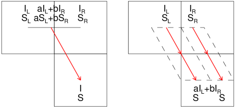
Figure 8: Short-characteristics step to get the intensity in the target cell (bottom) from the values at the previous cell plane (top) in two dimensions: left: standard integration with one short ray and interpolation of intensity and source function at the top grid plane; right: separate rays for each neighbor cell with a summing up of the intensity in the bottom grid cell, the splitting of each ray gives the intensity change within each cell.

The LC scheme described in the previous section is part of CO5BOLD since the very beginning. It is adapted to the conditions of plane-parallel atmospheres in local models: e.g., it heavily makes use of periodic side boundary conditions. The angular distribution of rays is chosen to optimize the vertical radiative flux. The diffusion approximation used in the deeper layers can save some computational time.

While for local models there was no reason to spend time on experimenting with another radiation-transport scheme, this changed for global models where the conditions are different: the vertical direction is not preferred anymore. Instead, all sides of the computational domain are open for radiation. The numerical resolutions is in general worse than for local models and the violent flows and give rise to large local temperature and opacity fluctuations. This means that errors caused by the interpolation in LC schemes would become more apparent.

The short-characteristics (SC) scheme in CO5BOLD overcomes these stability problems at the possible expense of the accuracy of the vertical radiative energy flux. The basic idea of not following rays through the entire volume is the same as in Kunasz and Auer [119]. But a different way of interpolating the intensity and the source function makes it better adapted to the use within an RHD code.

The main emphasis during the development of the SC scheme has been put on stability by preventing local peaks of the source function from “leaking” into neighbor cells and causing an unwanted smearing of the cooling or heating term (see Fig. 6). This requires a special reconstruction of the source function within optically thin cells in the 1D radiation transport operator and a carefully chosen interpolation within the SC scheme.

Instead of a Feautrier scheme as in Sect. 3.6.3, the analytic solution of the 1D version of the radiation transport equation (22) with linear source function (Fig. 7, left) is used as atomic operator,

$$I_{1}=I_{0}\,e^{-\Delta\tau}\,+\,S_{1}\,-\,S_{0}\,e^{-\Delta\tau}\,+\,\frac{\Delta S}{\Delta\tau}\left[e^{-\Delta\tau}-1\right]\enspace,$$ (66)

which guarantees the positivity of the source function everywhere.

The energy change has to be computed accurately in the optically very thick (e.g., in the center of a toy stellar model with $\Delta\tau>10^{8}$) and in the optically very thin (e.g., in some regions far away from the surface of a red supergiant model with $\Delta\tau<10^{-20}$). Both cases pose no problem for the formal solution because in the former case the intensity is essentially given by the local source function. And in the latter case, the changes to the radiation field due the contribution of the extremely thin regions can be safely ignored – or simply added to the much larger intensity along a ray and therefore absorbed by the limited machine precision. However, optically very thick or thin regions still interact with the radiation field and the local heating or cooling is significant and has to be computed in a time-dependent code. The SC scheme in CO5BOLD uses different arrangements of terms in optically thin and thick regimes to account for round-off errors, giving accurate values for optically very thick or thin regions – even running only in single precision.

Separate integration steps are employed for the interval from the cell center to the boundary and from the cell boundary to the next cell center (Fig. 7, right) to get the intensity change within each cell, from which the energy change per cell is computed. In the optically thin regime, the slope of the source function is reduced (Fig. 7, right) to suppress leaking of cooling or heating from one cell to the next (Fig. 6). Each ray inclination requires an integration of the intensity in both directions. For inclined ray directions, there is one pair of intensity-integration steps for each pair of neighbor cells to avoid the leaking of cooling or heating associated with the spatial interpolation of source function and/or intensity (Fig. 8). That means, that in contrast to the well-known SC scheme in Kunasz and Auer [119], even for a single direction there might be more than one ray connecting a cell with its neighbors.

The numerical scheme proceeds as follows:

At the beginning of each radiation-transport sub step, the temperature $T$ is computed from density $\rho$ and internal energy $e_{\mathrm{int}}$ for every mesh point of an equidistant 3D Cartesian grid. For every frequency group (Sect. 3.6.2) opacity $\kappa$ and source function $S$ are calculated by interpolating in precompiled tables. Next, for every ray inclination the optical thickness $\Delta\tau$ of each cell is calculated.

At the beginning of each integration step, the boundary values of the intensity have to be set. For the SC scheme, only open boundary conditions (zero infalling intensity) are implemented (for simulations with periodic side boundaries, the LC scheme (Sect. 3.6.3) is used, instead).

The integration proceeds then layer by layer along the axis that is closest to the inclined ray direction. For each ray direction, the intensity at each cell does not depend on its neighbors within a layer but only on cells in the previously computed layer. That means, that the innermost loop in each layer can be efficiently vectorized. The next loop is parallelized with OpenMP directives and the outermost loop performs the integration.

Each complete 3D radiation-transport step includes directions according to the coordinates of the corners of regular polyhedrons, which results in equal weights for all rays. After the loop over all inclinations and the loop over all frequency groups, the energy change per time is derived from all the accumulated intensity changes and used to update the internal energy $e_{\mathrm{int}}$ in each cell for given time step $\Delta t$. Here, “conservation of intensity” translates into “conservation of energy” and ensures the conservativity of the radiation-transport update step (except for the losses through the outer boundaries).

From one sub time step to the next, the orientation of the polyhedron can change randomly to give some coverage of the entire sphere. However, some simulations are restricted to rays aligned with axes or diagonals resulting in a considerable speed-up while loosing some angular resolution. There are several radiative time steps per hydrodynamics time step possible to compensate for the short radiative time scale compared to the hydrodynamic one.

In cool supergiants close to the Eddington limit, radiation pressure plays an important role in the stellar atmosphere and the wind of asymptotic giant branch (AGB) stars is driven by radiative pressure on dust. With the scheme presented above, the three components of the radiative acceleration can easily by computed from the intensity change per cell.

3.7 MHD

In CO5BOLD, the numerical scheme used for the solution of the equations of magneto-hydrodynamics is quite different from the one employed for the case of pure hydrodynamics described in Sect. 3.5. In the case of solar and stellar magnetoconvection, the scheme must be able to deal with highly stratified flows where the plasma-$\beta$ (i.e., the ratio of the thermal to the magnetic energy density of the plasma) varies over several orders of magnitude. A special requirement of MHD calculations is the enforcement of the divergence-free condition $\mathbf{\nabla}\cdot\mathbf{B}=0$ for the magnetic field. Violating this condition can lead to unphysical forces, which can degrade the solution [120]. Several methods have been developed to enforce this condition either to roundoff error or approximately to the order of the scheme. One method is to use the eight-wave formulation of the MHD equations [121, 122]. The additional wave is associated with the propagation of magnetic monopoles. In the eight-wave formulation, additional source terms proportional to $\mathbf{\nabla}\cdot\mathbf{B}$ appear, i.e., the equations are no longer conservative. Another method uses a cleanup step at the end of each time step, removing the errors in $\mathbf{\nabla}\cdot\mathbf{B}=0$. This requires the solution of a Poisson equation at each time step. A third possibility, which is used in the MHD module of CO5BOLD, is the constrained-transport method of Evans and Hawley [123]. It uses a special finite-difference discretization of the induction equation on a staggered grid such that a discrete formulation of the divergence-free condition for the magnetic field is maintained to machine accuracy. All of these methods can be treated as modifications of an underlying base scheme. A detailed comparison of these methods can be found in Tóth [124].

Another difficulty in MHD simulations is to keep the thermal gas pressure positive [125, 126]. Since the gas pressure is a dependent variable when using the conservative form of the MHD equations, it is computed by subtracting the potential, the kinetic, and the magnetic energy from the total energy, $e_{\mathrm{tot}}$. When the magnetic energy is much larger than the internal energy, i.e., for small values of the plasma-$\beta$, small errors in the total energy can drive the gas pressure to negative values. This can be a problem in the solar chromosphere, where values of $\beta\approx 10^{-4}$ are common, whereas the gas pressure dominates in the sub-photospheric layers where $\beta$ is huge. In the MHD module of CO5BOLD, several provisions are made to avoid a negative gas pressure. To keep the magnetic field solenoidal, CO5BOLD uses the constrained-transport method in combination with a Godunov-type finite-volume scheme as the base scheme. In the following, each component of the scheme is described in more detail.

3.7.1 Spatial and temporal discretization

The spatial discretization of the MHD equations is similar to the hydrodynamic case, i.e., the hydrodynamic variables are cell centered. The magnetic fields are located at the cell interfaces. The cell-centered magnetic field components, which are required by the Riemann solver of the base scheme, are computed from the magnetic field components at the cell interfaces by linear interpolation. Then all cell-centered variables are updated by the base scheme. The extension to second order in space is done by linear reconstruction of the primitive variables $\rho$, $\mathbf{v}$, $\mathbf{B}$, $P$, and $\rho e_{\mathrm{int}}$. Second order in time is achieved either by a Hancock predictor step [127, 128] or by a second-order TVD-Runge-Kutta time-integration scheme [129]. In some situations, where the second-order scheme would result in negative gas pressure, the scheme is locally reduced to first order.

3.7.2 The approximate Riemann solver

In the hydrodynamic scheme of CO5BOLD, a Roe solver is used (Sect. 3.5). However, the Roe solver does not guarantee positivity of the density and the pressure. This problem, which is also present in the hydrodynamic case gets worse for MHD. Whereas in the hydrodynamic case, reducing the time step often helps to overcome the problem, in MHD simulations, the problem remains, even if the time step is reduced considerably.

It can be shown that the HLL solver [130] ensures positivity of the gas pressure and the density if the exact solution of the Riemann problem is positive [131]. For MHD, this is the case only if there is no jump in the normal component of the magnetic field. In 1D, the divergence-free condition enforces the normal component of the magnetic field to be constant. For multi-dimensional problems however, using cell-centered magnetic fields, jumps in the normal component of the magnetic field occur even if the divergence-free condition is fulfilled in a discrete sense. It was shown by Janhunen [126] that allowing magnetic monopoles, which arise from these jumps, and taking into account their contribution to the Lorentz force, an additional source term occurs in the induction equation only. Using a special discretization of this source term, Janhunen [126] demonstrated numerically that the HLL solver for MHD always provides positive gas pressures.

We use the method of Janhunen for the MHD module of CO5BOLD. However, it should be noted that this source term is only used for the computation of the fluxes by the HLL-solver of the base scheme. For the update of the magnetic field by the constrained-transport method, this source term is not used so that the magnetic field stays divergence-free.

3.7.3 The constrained-transport step

CO5BOLD uses the flux-interpolated constrained-transport method of Balsara and Spicer [132]. First, the electric field at the cell edges is computed from the fluxes at the centers of the cell interfaces, provided by the base scheme. The magnetic field at the cell interfaces is then updated with this electric field, applying Stokes theorem to every face of a cell. The updated cell-centered magnetic field from the base scheme is discarded. The new cell-centered magnetic field is computed from the updated magnetic field at the cell interfaces by linear interpolation.

Since the new cell-centered magnetic field is different from the magnetic field provided by the base scheme, the internal energy, $e_{\mathrm{int}}$, must be modified after the constrained-transport step according to

$$e_{\mathrm{int}}=e_{\mathrm{int}}^{*}+\frac{\mathbf{B}^{*}\cdot\mathbf{B}^{*}-\mathbf{B}\cdot\mathbf{B}}{2\rho}\enspace,$$ (67)

where $\mathbf{B}^{*}$ and $e_{\mathrm{int}}^{*}$ are the magnetic field and the internal energy provided by the base scheme. If this correction would result in negative gas pressure, it is not performed, i.e., $e_{\mathrm{int}}=e_{\mathrm{int}}^{*}$ (see also Balsara and Spicer [132]) and the total-energy conservation is sacrificed in favor of improved robustness.

3.7.4 Dual-energy method and Alfvén-speed reduction

Even if a scheme guarantees positivity of the gas pressure, this does not necessarily mean that the gas pressure is computed accurately. In fact, by using the total energy equation for the computation of the internal energy, the discretization errors in the total energy, the kinetic energy, and the magnetic energy of the scheme tend to be imposed on the internal energy. One could use the entropy equation or the equation for the thermal energy itself, instead. Another possibility is to use the total energy equation in combination with one of these equations. For example Balsara and Spicer [125] use the entropy equation for the update of the internal energy in regions with strong magnetic fields. For the MHD module of CO5BOLD, the so-called dual-energy method, i.e., a combination of the equation for the total energy and the equation for the thermal energy is used. In regions with a large $\beta$, the internal energy is updated with the equation of the total energy. In turn, when $\beta$ is small ($\beta\lessapprox 10^{-3}$), the equation for the internal energy is used at the expense of strict energy conservation. Since typically $\beta$ is small in very restricted regions of the computational box only, conservation of total energy is still maintained in most parts of the computational domain.

In order to avoid extremely small time steps due to the CFL condition when the Alfvén speed is high, the Alfvén speed can be limited by artificially reducing the strength of the Lorentz force by a factor

$$f=\frac{v_{\mathrm{Amax}}^{2}}{v_{\mathrm{A}}^{2}+v_{\mathrm{Amax}}^{2}}\enspace,$$ (68)

where $v_{\mathrm{A}}$ is the actual Alfvén speed and $v_{\mathrm{Amax}}$ is the desired upper limit of the Alfvén speed. The method is similar to that used by Rempel et al. [133]. Of course, caution is indicated when using this method. Obviously, it can hardly be used for the study of magnetoacoustic wave propagation. However, it may be perfectly admissible in situations, where the low-$\beta$ regime is merely included as a buffer region to the (upper) boundary of the physical domain.

3.7.5 Ohmic diffusivity

While it is not necessary for stability, the MHD-scheme of CO5BOLD can also handle explicit magnetic diffusion. It is treated explicitly in the scheme by modifying the electric field in the constrained-transport-step. A constant magnetic diffusivity and the artificial magnetic diffusivity according to Stone and Pringle [134] are currently implemented in CO5BOLD. The constant magnetic diffusivity can be used to specify the magnetic Reynolds number

$$R_{m}=\frac{vL}{\eta}\enspace,$$ (69)

where $\eta$ is the magnetic diffusivity, $L$ is a typical length scale and $v$ is a typical velocity of the flow. The artificial magnetic diffusivity is given by

$$\eta=C\frac{\left(\Delta x\right)^{2}|\mathbf{j}|}{\sqrt{\rho}}\enspace,$$ (70)

where $\Delta x$ is the grid spacing, $\mathbf{j}=\mathbf{\nabla}\times\mathbf{B}$ is the current density, and $C$ is a dimensionless parameter.

3.7.6 Magnetic boundary conditions

The boundary conditions for the magnetic field can be specified independently from the hydrodynamic settings for the top and the bottom boundaries, and for each of the horizontal directions. Typical horizontal boundary conditions used for simulating magnetoconvection in a local box are periodic. Another boundary condition, mostly applied to the bottom and the top of the box, consists in setting the magnetic field tangential to the boundary to zero, so that the magnetic field lines stay normal to the boundary. A generalization of this boundary condition specifies the obliquity of the magnetic field at the boundary. There is also a special condition for the open lower boundary, which allows upflows to advect horizontal magnetic field into the computational box. Another boundary condition consists in setting the electric field to zero at the boundary. This means that the normal component of the magnetic field at the boundary does not change. In this case the magnetic field lines are effectively anchored at the boundary.

Conditions which keep the magnetic field vertical at the top and bottom boundaries are typically used for the simulation of intense, vertically directed magnetic flux tubes in the photosphere of the Sun as they occur in magnetically active regions such as plages and enhanced network regions. The advection of weak horizontal field across the bottom boundary is used for the simulation of magnetically inactive, very quiet regions on the Sun. With this boundary condition, it is assumed that convective updrafts transport magnetic fields from deep layers of the convection zone to the solar surface. Anchored fields may be useful for anchoring an entire sunspot at the bottom boundary or for anchoring horizontal fields at the side boundaries for the simulation of horizontally directed penumbral filaments.

3.8 Optional modules

The numerical treatment of the source terms $S_{i}$ in Eq. (29) dealing with different types of dust and chemical-reaction networks is implemented as a separate step (see below), following the general concept of operator splitting. The optional modules are called after the (magneto)hydrodynamics step for each computational time step. These modules treat the mass or number densities of the dust particles or chemical species as additional quantities, which are included in the in- and output of the simulation data. Only up to one of these extra modules can be used at a time, so far.

During the (magneto)hydrodynamics solver step, the additional densities are advected with the flow field analogously to the gas density. Their transport velocity across each cell boundary is computed from the gas mass flux divided by the upwind density, in some cases modified to account for the gravitational settling of dust.

The contribution of the additional components to the total opacity can be added to the standard equilibrium gas opacities (Sect. 3.6.2). The boundary conditions are made consistent with the hydrodynamics part of the code.

3.8.1 Chemical-reaction networks

Apart from advection across the cell boundaries, the number density $n_{i}$ of a chemical species in a grid cell can be changed due to chemical reactions:

$$\left(S_{i}\right)_{\mathrm{chem}}=-n_{i}\sum_{j}k_{2,ij}\ n_{j}\;+\;\sum_{j}\sum_{l}k_{2,jl}\ n_{j}n_{l}\;-\;n_{i}\sum_{j}\sum_{l}k_{3,ijl}\ n_{j}\ n_{l}\;+\;\sum_{j}\sum_{l}\sum_{m}k_{3,jlm}\ n_{j}\ n_{l}\ n_{m}$$ (71)

with the index $i$ for the included species. So far, the implementation is restricted to two- and three-body reactions, which is a reasonable assumption for comparatively hot stellar atmospheres. The losses (negative sign) and gains (positive sign) due to two-body reactions are described by the first and second right-hand terms with the corresponding reaction rates $k_{2,ij}$ and $k_{2,jl}$, respectively. Analogously, the third and fourth term describe the change due to three-body reactions. Such an equation is imposed for each included chemical species, resulting in a system of ordinary differential equations of first order. In CO5BOLD, the chemical reactions are handled locally for each grid cell separately by solving the system of differential equations. It starts with the calculation of the reaction rates $k$, which are functions of the local gas temperature and (for catalytic reactions) also of the number density of a representative metal. The influence of the radiation field has been neglected so far. The functions are parametrized with prescribed coefficients that are provided in the form of a table [see 135, for details].

The chemical-reaction rates, the number densities of the involved species, and thus their derivatives can differ by many orders of magnitude, which can cause the system of equations to be stiff. Thus, an implicit scheme is used for the numerical solution. We based our solver on the DVODE package [136] with an implicit BDF (backward differentiation formula) method and an automatic internal time step. The solution finally provides the number densities of the involved species after the overall (global) computational time step. For the numerical simulation of carbon monoxide, 7 chemical species and a representative metal are considered, which are connected through 27 chemical reactions [135].

Carbon monoxide is a non-negligible opacity source in the solar atmosphere, so that the opacity is in principle affected by the deviations from equilibrium of the CO number density. To account for this effect, the back-coupling to the radiative transfer was implemented [137]. It follows the approach by Steffen and Muchmore [138], which uses two frequency groups. The first comprises the gray Rosseland opacity $\kappa_{\mathrm{R}}$ without the wavelength region around the CO fundamental vibration-rotation band in the infrared at a wavelengths around $\sim 4.6~{}\mu\mathrm{m}$. This wavelength range is simulated with the second band, which is constructed from the gray Rosseland opacity $\kappa_{\mathrm{R}}$ and an additional opacity $\kappa_{\mathrm{CO}}$. The latter is directly connected to the CO number density that is derived from the preceding solution of the chemical-reaction network.

3.8.2 Time-dependent hydrogen ionization

A detailed treatment of the time-dependent ionization of hydrogen is important for atmospheric layers, where significant deviations from the ionization equilibrium occur, e.g., in the solar chromosphere (see Sect. 4.5). Current applications for the Sun use a hydrogen model atom with 5 bound energy levels and a level representing ionized hydrogen. The number densities of the individual level populations $n_{i}$ enter as additional quantities in CO5BOLD. The levels are connected by collisional transitions and 10 radiative transitions (5 bound-bound and 5 bound-free). The rate $P_{\ij}$ of a transition between a level $i$ and a level $j$ is given by $P_{\ij}=C_{\ij}+R_{\ij}$, where $C_{\ij}$ and $R_{\ij}$ are the rates due to collisional and radiative transitions, respectively. First, these rates are calculated from the local gas density and gas temperature, the imposed radiation field, and the level populations and electron densities, that are available from the previous time step. Apart from advection, the change of the population number densities and thus the ionization degree of hydrogen in a grid cell is then described by a set of time-dependent rate equations of the form

$$\left(S_{i}\right)_{\mathrm{hion}}=\sum_{j\neq i}^{n_{l}}n_{j}P_{ji}-n_{i}\sum_{j\neq i}^{n_{l}}P_{ij}\enspace,$$ (72)

where the terms on the right-hand side are the rates into and out of level $i$. In CO5BOLD, the set of rate equations for all considered energy levels is solved with the DVODE package like that for the chemical-reaction networks (see Sect. 3.8.1).

An important simplification concerns the usage of fixed radiative rates. In principle, the radiation field and the radiative transitions for hydrogen (both bound-bound and bound-free) are connected in such a way that a detailed solution has to be found by iteration, which makes it computationally expensive. For the implementation in a multi-dimensional radiation MHD code, the rates are fixed and calibrated so that they reproduce the full solution as it is implemented in time-dependent 1D simulations [139, 140]. There is no back-coupling to the equation of state and the opacities in the current implementation in CO5BOLD, a point, which will be worked on in the future. More details are given in Leenaarts and Wedemeyer-Böhm [141].

3.8.3 Dust

If the atmospheric temperatures are low enough, not only molecules but larger particles – dust – can form. In the Earth’s atmosphere, possible types of such particles are for instance aerosols of different compositions, rain, snow, or hail, mostly made of water, or particles from volcanic ashes. Many cool stars or substellar objects may contain dust in their atmospheres, too (see Fig. 11). In the hotter objects, the dust will mostly be made of minerals (e.g., forsterite). At lower temperatures (e.g., on the Earth) water plays an important role. For the dust chemistry of the warmer objects, it is crucial whether oxygen or carbon is more abundant, because these two elements first form carbon monoxide gas (CO) and only the remainder participates in dust formation. The formation, interaction, and destruction of grains of different chemical composition, size, and shape is difficult to model [142, 143]. Compared to the possible complexity of the processes occurring in real objects, the various dust modules in CO5BOLD are simple. They are permanently under development. Two examples will be outlined in the following:

Stars at the tip of the asymptotic giant branch lose part of their mass in form of a stellar wind, likely driven by radiation pressure on dust. The formation of carbon-rich dust around such stars was investigated by Freytag and Höfner [144] with CO5BOLD and with the 1D-RHD code of Höfner et al. [107]. The CO5BOLD dust model includes a time-dependent description of dust grain growth and evaporation using a method developed by Gail and Sedlmayr [145] and Gauger et al. [146]. In this approach, the dust component is described in terms of four moments $K_{j}$ of the grain-size distribution function, weighted with a power $j$ of the grain radius. The moment $K_{0}$ represents the total number density of grains (integral of the size distribution function over all grain sizes), while the ratio $K_{3}/K_{0}$ is proportional to the average volume of the grains. The equations, which determine the evolution of the dust components, are solved considering spherical grains consisting of amorphous carbon. The nucleation, growth, and evaporation of grains is assumed to proceed by reactions involving C, C₂, C₂H, and C₂H₂. The four moments $K_{j}$ are number densities and are advected with the gas as described in Sect. 3.8. The gas and dust opacities in this case are gray. Some results are shown in Sect. 4.7 and Fig. 15.

In contrast to the cool giants, the conditions for the formation of (oxygen-rich) dust in M dwarfs and brown dwarfs are fulfilled even in standard 1D atmosphere models. However, the comparatively heavy dust grains should sink under the influence of gravity and vanish from the visible photosphere, leaving no direct trace in emergent spectra, which is at variance with observations. The scheme used in [96] to investigate the question why the dust does not settle or how the material comes back up is based on a simplified version of the dust model used in [107], adapted to forsterite (Mg₂SiO₄, 3.3 g/cm³). In this method, there are only two density fields, one is used to specify the mass density of dust particles and the other to describe the monomers (the dust constituents), instead of four density fields for the dust and none for the monomers as in [107] and [144]. Therefore, the ratio of the sum of dust and monomer densities to the gas density is allowed to change, in contrast to the dust description in [107] used for the AGB simulations mentioned above. Instead of modeling the nucleation and the detailed evolution of the number of grains, a constant ratio of the number of seeds (dust nuclei) to the total number of monomers (in grains or free) per cell is assumed. If all the material in a grid cell were to be condensed into dust, the grains would have the maximum radius $r_{\mathrm{d,max}}$, which is set to a typical value of 1 $\mu$m. This is close to the typical particle sizes found for the optically thick part of the cloud deck in solar-metallicity brown dwarfs according to the DRIFT-PHOENIX models of Witte et al. [147].

Condensation and evaporation are modeled as in [107], with parameters and saturation vapor curve adapted to forsterite. In the hydrodynamics module, monomers and dust densities are advected with the gas density, with the terminal velocities given by the low-Reynolds-number case of Eq. (19) in Rossow [148] as settling speed added to the vertical advection velocity of dust grains. In contrast to the sophisticated treatment of the gas opacities, a simple formula for the dust opacities is used, which assumes that the large-particle limit is valid for all grain sizes and treats scattering as true absorption. The dust opacity in each cell of the simulated atmosphere is added to the gas opacity (Sect. 3.6.2). Experiments have been made with another dust model, that uses in addition to one density field for the monomers a number of further fields, one for each possible grain size.

4 Results

4.1 Code comparison: the solar benchmark

Table 1: Setup and emergent radiation of solar models computed with different codes.

	STAGGER	MURaM	CO5BOLD	CO5BOLD
			standard	high resolution
Box size [Mm3] ($x\times y\times z$)	$6.0$$\times$$6.0$$\times$$3.6$	$9.0$$\times$$9.0$$\times$$3.0$	$5.6$$\times$$5.6$$\times$$2.3$	$5.6$$\times$$5.6$$\times$$2.3$
Grid dimension	$240$$\times$$240$$\times$$230$	$512$$\times$$512$$\times$$300$	$140$$\times$$140$$\times$$150$	$400$$\times$$400$$\times$$300$
Cell size [km3] ($\Delta x\times\Delta y\times\Delta z$)	$25.1$$\times$$25.1$$\times$$\Delta z^{\ast}$	$17.6$$\times$$17.6$$\times$$10.0$	$40.0$$\times$$40.0$$\times$$15.1$	$14.0$$\times$$14.0$$\times$$7.5$
Height range [Mm] ($z=0$ at $\langle\tau\rangle=1$)	$-2.72\ldots+0.88$	$-2.00\ldots+1.00$	$-1.38\ldots+0.88$	$-1.38\ldots+0.88$
upper boundary condition	transmitting	closed	transmitting	transmitting
lower boundary condition	open	open	open	open
# snapshots used	$19$	$19$	$19$	$60$
# frequency groups used	$12$	$4$	$12$	$12$
Effective temperature [K]	$5762$	$5768$	$5781$	$5763$
Bol. intensity contrast ($\mu$=1) [%]	$14.9$	$15.4$	$14.4$	$14.1$

^∗ The STAGGER code uses a non-equidistant grid in the vertical direction, with spacings ranging from $\Delta z=7$ km near the optical surface to $\Delta z=32$ km in the deepest layers.

The natural benchmark for the comparison of different codes is of course the solar atmosphere. On the one hand, its mean thermal stratification is well known empirically, and its velocity field and associated temperature fluctuations have been studied in great detail based on a large body of observations. On the other hand, many numerical simulations have been carried out to study solar surface convection with a variety of different computer codes. Here, we compare some basic quantities obtained from numerical simulations of the solar surface layers with three different codes: STAGGER, MURaM, and CO5BOLD. All three codes solve the time-dependent equations of compressible (magneto)hydrodynamics for a gravitationally stratified, radiating fluid in a Cartesian box in 3 spatial dimensions, taking into account partial ionization and non-gray radiative energy exchange, the latter treated with the opacity-binning scheme (see Sect. 3.6.2).

The codes have been developed independently and use different numerical methods. STAGGER and MURaM are similar in that both use a method of lines for the hydrodynamics part as well as artificial (hyper)diffusivities to stabilize the numerical solution. The STAGGER code [59], [149] (see also Sect. 1) uses a sixth-order finite-difference method to determine the spatial derivatives on a staggered mesh, while the equations are stepped forward in time using an explicit third-order predictor-corrector procedure, conserving mass, momentum, energy, and magnetic-field divergence. Radiative energy exchange is found by the formal solution of the Feautrier equations on long rays. Similarly, MURaM [150], [54] uses a fourth-order central-difference scheme in space, and a fourth-order Runge-Kutta time stepping; radiation transport is computed with a short-characteristics method. On the other hand, CO5BOLD is based on a finite-volume approach and employs an approximate Riemann solver of Roe type to advance the hydrodynamics in time, relying on second-order monotonic reconstruction schemes to achieve numerical stability without the need to invoke artificial viscosities. Directional splitting reduces the 3D problem to one dimensional sub-steps. Similar to STAGGER, radiative transfer is treated with a Feautrier method on long characteristics (see Sect. 3.6.3).

The basic setup of the different solar simulation runs is summarized in Table 1. The two CO5BOLD models differ only in their spatial resolution. Since the models of the different groups have not been constructed for the purpose of this comparison, they differ in many aspects, such as horizontal box size, vertical extent, spatial resolution, boundary conditions, opacity tables, number of frequency groups, and equation of state (EOS), apart from the different numerical methods used to solve the equations of hydrodynamics and radiative transfer. Despite these substantial differences, the mean vertical structure, obtained from the various simulations by horizontal and temporal averaging, turns out to be remarkably similar, as demonstrated in Fig, 9. Obviously, the mean thermal structure is the most robust quantity. Ignoring the layers influenced by the top boundary, the temperature differences are everywhere below 2%; deviations seen in the deeper layers are probably related to differences in the EOS. Except for the photospheric layers above $\approx 300$ km, where the details of the opacity-binning recipe play a major role, the predicted amplitude of the horizontal temperature fluctuations is also amazingly similar. As a consequence, the predicted continuum-intensity contrast (see Sect. 4.2) is found to be in very good agreement (last row of Table 1).

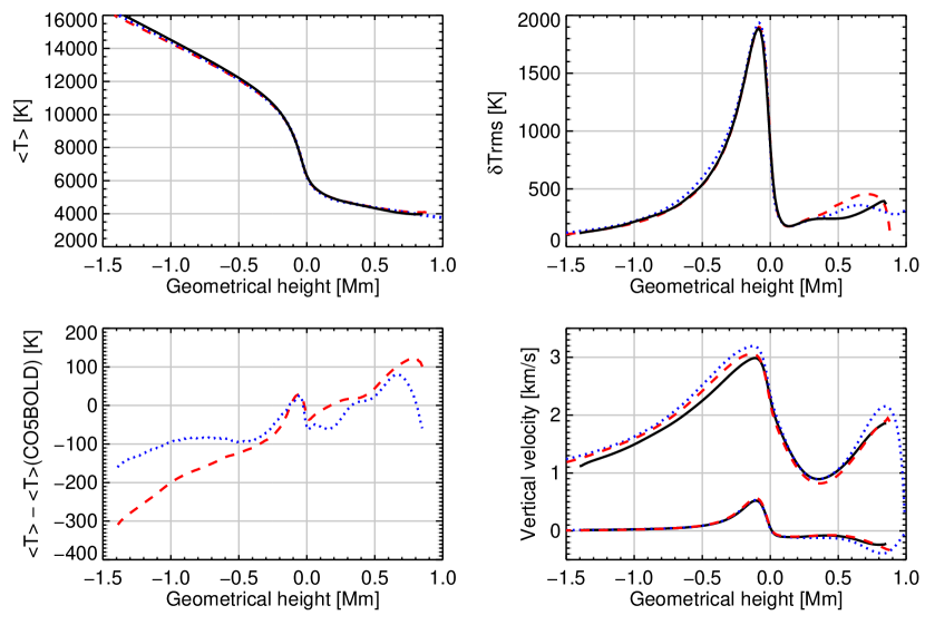
Figure 9: Comparison of the average vertical temperature structures, $\langle T\rangle(z)$ (left panels), the rms horizontal temperature fluctuations $\delta T_{\rm rms}=\sqrt{\langle T^{2}\rangle(z)-\langle T\rangle^{2}(z})$ (top right), and the mean and rms vertical velocity $\langle V_{z}\rangle(z)$, and $\sqrt{\langle V_{z}^{2}\rangle(z)}$, respectively (lower and upper set of curves in bottom right panel, respectively), as obtained with different codes for the solar simulations described in Table 1: STAGGER (dashed), MURaM (dotted), CO5BOLD standard (solid). Here $\langle.\rangle$ denotes averaging over horizontal planes of the numerical grid (constant geometric height $z$) and over selected snapshots in time.

The depth-dependence of the mean vertical velocity obtained from the three different simulations agrees closely (lower set of curves in lower right panel of Fig, 9). As theoretically expected, $\langle V_{z}\rangle$ is positive in the convectively unstable layers below the surface, and negative in the overshoot region. Somewhat larger deviations among the different models are found in the velocity dispersion, $\sqrt{\langle V_{z}^{2}\rangle(z)}$ (upper curves). Is seems that both the location of the lower boundary and the spatial resolution have some influence on the resulting velocity amplitude. Nevertheless, the overall agreement is very satisfactory.

We have to keep in mind that the different codes are largely based on the same physical assumptions and approximations. It may therefore not be too surprising that the resulting atmospheric structures are similar. And it does not prove that all details of the models are physically correct.

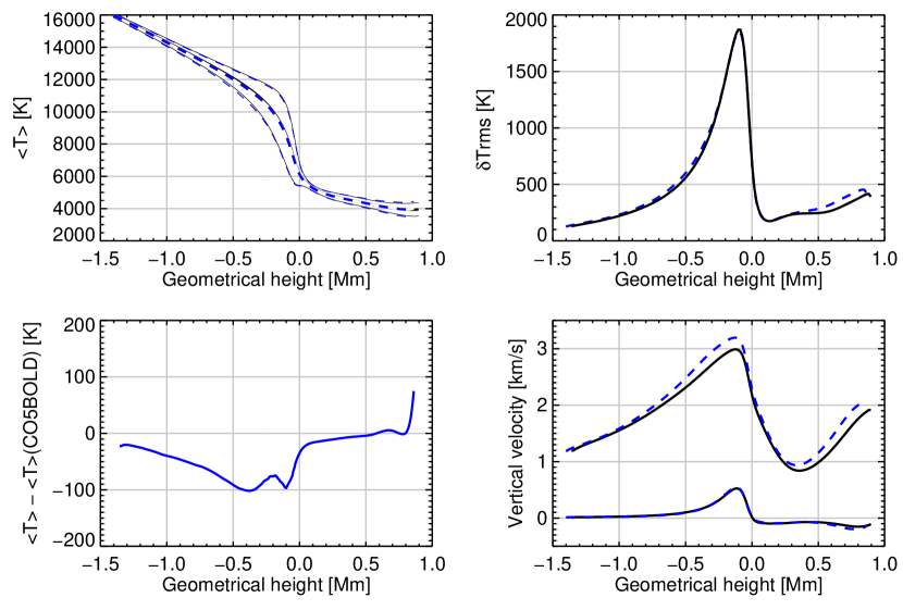
Figure 10: Comparison of the same quantities as in Fig. 9, but for two CO5BOLD solar simulations which differ only in spatial resolution: CO5BOLD standard (solid) and CO5BOLD high resolution (dashed). The thin curves in the upper left panel refer to $\langle T\rangle(z)\,\pm\,\delta T_{\rm rms}(z)$.

The role of the spatial resolution is illustrated in Fig. 10, where we compare two CO5BOLD models that differ only in spatial resolution: in the high-resolution model (cf. Fig. 1), the horizontal cell size is reduced by a factor $2\,\sqrt{2}$ with respect to the standard CO5BOLD model, while the vertical cell size is reduced by a factor of $2$. The mean thermal structure is practically unchanged, as is the amplitude of the T-fluctuations up to the mid photosphere. As a consequence, the intensity contrast is not significantly affected by the increased grid resolution (see Table 1). However, in the upper photosphere above $z\approx 300$ km, the amplitude of both the temperature and velocity fluctuations increases somewhat with increasing spatial resolution. The question whether the moderate spatial resolution of the standard hydrodynamical models is fully sufficient to account for the “turbulent” character of the solar photosphere, and hence for correctly capturing the non-thermal Doppler broadening of spectral lines, is currently under investigation. Obviously, this is an important issue in the context of accurate chemical abundance determinations based on 3D model atmospheres (cf. Sect. 4.3).

4.2 Granular intensity contrast

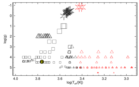
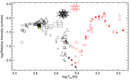
Figure 11: Top: grid of CO5BOLD models in the $\log T_{\mathrm{eff}}$-$\log g$ diagram. Bottom: logarithm of rms bolometric intensity contrast versus $\log T_{\mathrm{eff}}$. The squares mark 3D local models, the triangles 2D local models. The stars indicate global models (with very low surface gravity). Larger symbols indicate lower gravity. The Sun has its own standard symbol $\odot$ with yellow background. A red symbol (at lower effective temperatures) shows that some treatment of dust is included in the simulation.

The granulation pattern visible at the solar surface is a manifestation of convection in the sub-photospheric layers: bright granules correspond to hot rising gas, while the dark intergranular lanes consist of cooler downward-sinking material. The relative continuum-intensity contrast,

$$\delta I_{\rm rms}={\left\langle\frac{\sqrt{\langle I(x,y,t)^{2}\rangle_{x,y}-\langle I(x,y,t)\rangle^{2}_{x,y}}}{\langle I(x,y,t)\rangle_{x,y}}\,\right\rangle_{t}}{}\enspace,$$ (73)

of this granulation pattern and its variation from the centre of the solar disk to its limb are important tests for the degree of realism of numerical models. For many years, the values derived from observations were significantly lower than those calculated on the basis of numerical simulations [e.g., 151]. Recently, it was shown that synthetic continuum-intensity maps based on CO5BOLD [152] and also the code by Nordlund and Stein [149] can indeed reproduce the empirical values quite well, if the instrumental image degradation is taken into account properly [153]. The necessary image reconstruction is a very demanding task, which on the other hand turns out to be crucial, as was shown for observations obtained with the Solar Optical Telescope (SOT) onboard the Hinode satellite [154]. Hirzberger et al. [155] find very good agreement between the rms contrast of solar granulation obtained from measurements with a balloon-borne 1-m solar telescope and simulations at wavelengths of 388 nm and 312 nm. At shorter wavelengths, discrepancies between observations and simulations seem to persist.

By analogy, the surface of cool stars must be covered by a similar pattern, the stellar granulation. Its intensity contrast cannot be measured directly. Numerical simulations are necessary to infer how the intensity contrast depends on the stellar parameters: the effective temperature $T_{\mathrm{eff}}$, the surface gravity $\log g$, and the chemical composition.

The top panel in Fig. 11 shows the CO5BOLD models on the main sequence and above it (i.e., with gravities around $\log g$ 4 to 5 and lower: white dwarf models are not plotted) in a $\log T_{\mathrm{eff}}-\log g$ diagram. The displayed models comprise the solar-metallicity part of the CIFIST grid of solar-like 3D models [156], 3D M-dwarf models [157], local 2D “dusty” brown dwarf models [96], global 3D red supergiant [158, 159, 160] and AGB star models [144], as well as more experimental models of e.g., A-type stars (in 2D or 3D) and cepheids (in 2D). Larger symbols mean lower gravity (and usually a larger stellar radius). Squares depict 3D models, triangles 2D models. Solar models have the $\odot$ symbol. Global 3D models of red supergiants and AGB stars are marked as star symbols at the top. Red symbols indicate that the simulations have accounted for dust in some form. Models with non-solar metallicities are not shown.

The bottom panel shows the (bolometric) relative intensity contrast according to Eq. (73) versus $T_{\mathrm{eff}}$ for the same models and with the same symbols as in the top panel. On the main sequence (smallest symbols), the contrast decreases for stars cooler than the Sun since the stellar energy flux decreases and convection can transport it with smaller temperature fluctuations. The contrast does not increase further but has a plateau for stars a bit hotter than the Sun because convection does not carry the entire stellar flux anymore. Below a minimum at around 2600 K, the contrast increases again because fluctuating dust clouds start dominating the surface contrast (see Sect. 4.6). The contrast decreases at the very cool end due to the decreasing overall flux.

In general, lowering the gravity has a similar effect as increasing the effective temperature, but results in slightly more vigorous convective flows. The largest surface contrast is seen in the global AGB-star models, followed by the global red-supergiant models. 2D models have a larger contrast than 3D models. Other types of dust (and/or dust schemes) as well as global fluctuations might change the picture for the cooler models.

4.3 Solar and stellar abundances

One important application of multi-dimensional (multi-D) radiation-(magneto)hydrodynamics models is the determination of chemical abundances in late-type stars. Under most circumstances, information about the thermal and kinematic structure of a stellar atmosphere is necessary to interpret measured strengths of spectral lines in terms of chemical abundances. To this end, simulated time series of the evolution of the stellar photospheric flow field are serving as input for detailed spectral-synthesis calculations. The result of these calculations are time series of spatially resolved synthetic spectra which, after suitable averaging in space and time, can be compared to the observations. For CO5BOLD, we developed the spectral-synthesis code Linfor3D [161] which is on the one side adapted to the particular data formats and structures of CO5BOLD, and on the other side designed to facilitate the abundance analysis.

Historically, the application of multi-D models for deriving abundances started out on the Sun already early on. However, in the beginning mainly structural properties of surface convection and associated magnetic fields were in the modeling focus so that abundance analyses with multi-D models remained sparse. A turning point came with the work of Asplund and collaborators [162, 163] suggesting that multi-D effects are important in the Sun and metal-poor stars if one wishes to obtain high-fidelity abundances. Since then efforts are directed towards improving multi-D modeling aspects specific to abundance analysis work, and extending the model basis covering successively larger regions of the Hertzsprung-Russell diagram [156].

Hitherto, CO5BOLD models were applied to derive abundances of twelve elements in the Sun (see Caffau et al. [33] and references therein) including the CNO elements, which are important for the overall solar metallicity; work on further elements is in progress. In the field of metal-poor stars, CO5BOLD models were used to derive abundances from atomic (e.g., [164, 165]) as well as molecular lines (e.g., [166, 167]). An element of particular interest in metal-poor stars is lithium due to its connection to nucleosynthetic processes in the big bang and early universe. The lithium abundance is commonly derived from the Li I resonance line at 6707 Å. Since lithium is mostly ionized in the stars of interest, the formation of the line is highly temperature sensitive, which makes the resulting abundances strongly model-dependent. Hoping for lithium abundances of higher fidelity, multi-D models were rather extensively applied. CO5BOLD models were used to obtain lithium abundances in the most metal-poor dwarf stars known [168], to investigate the structure of the so-called “Spite plateau” at lowest metallicities [169], and to study the evolution of lithium in the globular cluster NGC 6397 [170]. A related aspect is the abundance ratio between the lithium isotopes ⁶Li/⁷Li in metal-poor stars. CO5BOLD models were applied to argue against claims of a non-zero isotopic ratio [34, 171]. The aforementioned investigations focused on dwarf or subgiant stars. There are also ongoing efforts to extend the application of CO5BOLD simulations to giant stars including studies of their abundances [172, 173, 174].

Besides conducting actual abundance analyses, CO5BOLD models were instrumental in a number of studies more indirectly linked to the derivation of stellar abundances from spectroscopy: the long-lasting issue of how small-scale velocity fields in stellar atmospheres give rise to the spectroscopically derived microturbulence [175, 157], and the influence of thermal inhomogeneities on effective temperatures derived from Balmer-line profiles [176].

The application of multi-D models to stellar-abundance studies is in its early stages and modeling challenges still exist: the need for a precise thermal structure of the optically thin, line-forming regions demands for a detailed representation of the radiation field. Sufficient wavelength resolution (Sect. 3.6.2), and inclusion of scattering processes are current challenges in the simulations proper. In the post-processing, line-formation calculations including departures from LTE are necessary to fully exploit the model potentialities but are demanding in terms of computational resources and amount of necessary atomic input data.

4.4 The magnetic Sun

4.4.1 Current status

Figure 12 exemplifies the type of MHD applications that are currently performed with CO5BOLD. It illustrates the magnetic field structure at the interface between the convection zone and the overlying atmosphere of the Sun. The top panel shows a close-up of a vertical cross section through the three-dimensional computational domain, where colors represent the magnetic field strength and arrows the velocity field. The dashed yellow/white curve indicates optical depth unity, i.e., the “solar surface” as seen in the visible part of the spectrum. Below this surface, the atmosphere is convectively unstable and energy is transported mainly by convection. Above this surface adjoins the stably stratified photosphere, where energy is mainly transported by radiation and where convective overshoot motions are rapidly damped. The panels in the bottom row show horizontal cross sections of corresponding size at three selected height levels and the emerging bolometric intensity in the rightmost panel (intensity map). The location of the vertical cross section is indicated by the dashed horizontal line in the bottom panels.

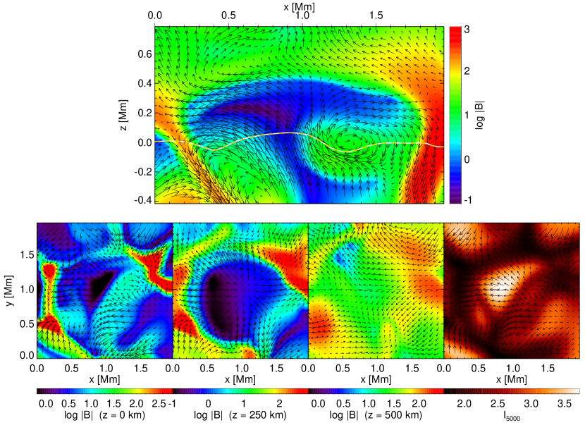
Figure 12: Flux expulsion in a close-up from a simulation of solar magnetoconvection: Logarithmic magnetic field strength in a vertical cross section (top) and in three horizontal cross sections (bottom) at heights of 0 km, 250 km, and 500 km. The emergent intensity is displayed in the rightmost panel. The arrows represent the velocity field projected in the respective coordinate planes. The yellow/white curve in the top panel marks the height of visible optical depth unity, i.e., the “solar surface”. From Wedemeyer-Böhm et al. [177].

We can see a strong central updraft in the vertical cross section of Fig. 12, which corresponds to the central granule visible in the intensity map. This granule is a typical representative for real solar granulation with respect to intensity contrast and size. Since the diffusion length scale of the magnetic field is small compared to the size of a granule, it is useful to think of the magnetic field to be “frozen into the plasma” so that the flow field transports the magnetic field from the granule center to its boundaries where it gets concentrated. This process is called the flux expulsion process, as magnetic flux is expelled from the granule interior to its boundaries. Correspondingly, the magnetic field in the central part of the granule is weak (dark blue) and it gets concentrated in the intergranular lanes (red), where plasma flows back into the convection zone again.

As the updraft runs into the stable stratification of the photospheric layer, it loses the driving buoyancy force and buoyancy starts to act in the opposite direction. Consequently, and also because of the strong density stratification, the flow must deviate in the horizontal direction and it drags the magnetic field with it as a consequence of the frozen-in condition. Hence, the magnetic field assumes a predominantly horizontal direction in the upper part of the photosphere, above the mushroom shaped void in Fig. 12 (top panel). While MHD simulation have since long predicted the existence of this prevalently horizontal field [178], it is only very recently that it got observationally detected with polarimetric measurements from the Hinode space observatory [179]. More details about MHD simulations with regard to this horizontal field can be found in Schüssler and Vögler [180], Steiner et al. [181], and Steiner et al. [182].

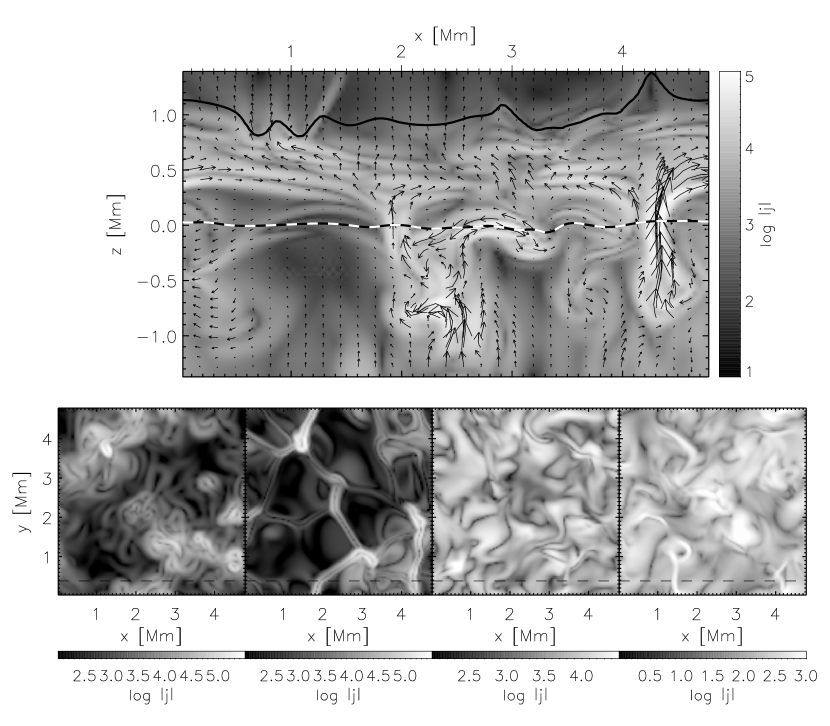
Figure 13: Logarithmic current density, $\log|j|$, in a vertical cross section (top panel) and in four horizontal cross sections (bottom panels) in a depth of 1180 km below, and at heights of 90 km, 610 km, and 1310 km above the mean surface of optical depth unity from left to right, respectively. The arrows in the top panel indicate the magnetic field strength and direction. The dashed line in the bottom row indicates the position of the vertical section. $j$ is given in units of $3\,\times\,10^{5}$ A/m². From Schaffenberger et al. [183].

Figure 13 shows the electric current density, $\mathbf{j}=\mathbf{\nabla}\times\mathbf{B}$, that forms as a consequence of the process discussed above, in a similar but larger domain than that of Fig. 12. Again, the top panel is a vertical cross section through the simulation domain, and the bottom row shows four horizontal cross sections at various heights. The magnetic flux concentrations in the intergranular lanes, which form as a consequence of the flux expulsion process, give rise to the conspicuous pairs of current sheets, visible in the horizontal cross section at $z=90$ km. Another system of current sheets forms in the region of predominantly horizontal magnetic fields above granules, in a height range from approximately 400–900 km, as can be seen from the vertical cross section. Higher up in the atmosphere, shock waves form where the supersonic plasma flow sweeps magnetic field into the compression zone downstream of and along the shock front. There again, current sheets form, e.g., the one extending from $x=1.1$ to $x=1.5$ Mm in the top part of the vertical cross section, which is also visible as a thin filament at $x=1.4$ Mm in the rightmost panel which corresponds to $z=1310$ km. More details about MHD simulations with CO5BOLD with regard to chromospheric shock waves can be found in Schaffenberger et al. [53] and Schaffenberger et al. [183]

Interestingly, the mean vertical Poynting flux, $\langle S_{3}\rangle$, where $\mathbf{S}=\mathbf{B}\times(\mathbf{v}\times\mathbf{B})=\mathbf{B}^{2}\mathbf{v}-(\mathbf{v}\cdot\mathbf{B})\mathbf{B}$ is all of the magnetic contribution to the total energy flux (see Eq.(19)), changes sign near optical depth unity. Below this depth, in the convection zone, the intense downdrafts in the intergranular lanes pump magnetic fields in the downward direction—cool and dense plumes compress and drag the magnetic field with them. This leads to a net Poynting flux in the downward direction. Above $\tau_{c}=1$, the Poynting flux that is connected to the magnetic field carried by the convective overshoot prevails, leading to a net Poynting flux in the upward direction. We expect that at least a part of this flux is turned into heat via ohmic dissipation by the current sheets that form on top of the overshoot in the chromospheric layers (see Fig. 13).

One purpose of performing realistic simulations is the synthesis of observable quantities from the simulation data, which then become directly comparable to actual observations of the Sun. This typically involves the integration of the radiation transfer equation along lines of sight across the computational domain in order to obtain (two-dimensional) synthetic intensity maps. This analysis step is performed post factum, after completion of the simulation. In case of magnetohydrodynamics, it requires the integration of the Unno-Rachkovsky equation for polarized radiation for obtaining intensity maps of the Stokes parameters. For direct comparison with observations from space-based or ground-based observatories, application of the corresponding instrumental point spread-function is necessary for degrading the synthetic intensity maps to the spatial resolution limits of the actual observation. Degradation in frequency space and addition of noise may be required for taking into account the frequency resolution of the spectrometer and the photon noise of the recording device, respectively. Quantitative comparisons of synthesized spectropolarimetric maps from CO5BOLD simulation data with corresponding intensity maps from the Hinode space observatory were performed by Steiner et al. [181] who focus on the above discussed horizontal magnetic fields and by Rezaei et al. [184] with respect to intergranular magnetic flux concentrations.

MHD simulations with CO5BOLD are also performed for studying the excitation and propagation of magnetoacoustic waves in the magnetically structured solar atmosphere. Effects of mode conversion, refraction, and transmission are studied for application in solar atmospheric seismology [185, 186, 187, 188].

4.4.2 Next steps

Most if not all simulations of stellar magnetoconvection rely on the MHD approximation. But the plasma in the photosphere of the Sun is weakly ionized so that the frozen-in condition may not really apply after all, despite the large scales of the magnetoconvective processes under consideration [see, e.g., 189, 190]. In the tenuous plasma of the chromosphere and corona, effects become important which are not included in the single-fluid model of the standard MHD equations, and a multi-fluid model or even a kinetic description of the plasma may become necessary.

Two consequences of a multi-fluid description are the Hall effect and the ambipolar diffusion. Since the electrons and ions are moving on curved trajectories between collisions, the current density vector is no longer colinear with the electric field vector, i.e., the electric conductivity is a tensor. Ambipolar diffusion occurs in partially ionized plasmas, where collisions between charged and neutral particles produce new diffusion mechanisms. Since only the charged particles are coupled to the magnetic field, the forces acting on the different particles are different. This leads to a drift between charged and neutral particles modifying the transport of magnetic flux in the plasma.

In the limit of a weakly ionized plasma consisting of electrons, ions, and neutrals, the single fluid description can still be applied along with an appropriate modification of the induction equation. This modification includes a term representing the Hall effect and a term representing the ambipolar diffusion. We plan to implement an optional inclusion of these terms in the computation of the numerical fluxes for the induction equation of CO5BOLD.

Ohmic dissipation of electric currents is probably the most important process in the heating of the outer solar atmosphere. In the present version of the MHD module of CO5BOLD, there is only an explicit implementation of a turbulent subgrid-scale magnetic diffusion (see Sect. 3.7.5). However, for taking a significant resistivity into account, an implicit treatment must be implemented. Also the occurrence of anomalous resistivity should be accounted for.

Currently, a much discussed topic in solar physics is the origin of the ubiquitous weak magnetic field outside sunspots. It is thought to be generated through induction due to the turbulent motion of the plasma near the solar surface, viz., by the turbulent dynamo [191]. On the other hand, turbulent pumping transports this magnetic field in the downward direction, away from the surface into the deep, less turbulent layers of the convection zone [192]. It is unclear, which effect prevails. First MHD simulations have been designed and carried out with the aim to improve our understanding of this riddle (Vögler and Schüssler [193], Moll et al. [194]). For a review see Stein [195] who argues that the solar dynamo has no preferred scale but rather acts throughout the convection zone over a wide range of scales.

Regarding global models of solar magnetohydrodynamics, the long term goal should be the global, three-dimensional, numerical simulation of the entire solar convection zone including at least the overshoot layers and a proper radiative transfer at its boundaries, but ideally also photosphere, chromosphere (see below), and corona. Thus, we seek a “Sun simulator” as a laboratory for the holistic simulation of the Sun on scales from the stellar radius to the size of granules of about 1000 km. The outcome should be a virtually self-consistent simulation of the differentially rotating convection zone including the self-exciting dynamo, which is thought to be at the origin of solar magnetic activity. Simulations should shed light on the functioning of the dynamo, the solar rotation law, the torsional oscillation, the luminosity variability, the sunspot cycle, and the global solar oscillation. Despite the apparent sphericity of stars, these processes are truly three-dimensional and therefore, they require a three-dimensional treatment unlike the traditional one-dimensional approach in stellar-evolution modeling.

The development of such a simulation tool is a formidable task (see Sect 2.1). The main challenge at the beginning consists in the recognition of the relevant physics to be included and in finding the proper physical approximations, numerical scheme, and adaptive meshing for achieving sufficient spatial resolution. So far, global MHD simulations have not been carried out with CO5BOLD. However, with CO5BOLD it should be possible to collect first experiences on the way to a true “Sun simulator”.

4.5 Solar chromosphere

The chromosphere is the thin atmospheric layer between the photosphere and the transition region and corona above. Although these layers are coupled by magnetic fields and waves, the properties of the atmospheric gas differ significantly. Compared to the photosphere below, the chromospheric gas is relatively thin, which has a number of important implications for the modeling (see Sect. 4.5.1) and also for observations. There are only a few diagnostics suitable for probing the chromosphere, which makes it hard to derive constraints and viable reality checks for numerical models. Even worse, the interpretation of most of these diagnostics is complicated by the fact that non-equilibrium effects must be taken into account. Advances in instrumentation both for ground-based and space-borne observations during the recent years made it nevertheless possible to access the dynamic and intermittent fine structure at small spatial scales like it is seen in current chromosphere simulations (see, e.g., the review by Wedemeyer-Böhm et al. [177]). The coexistence of magnetic fields and propagating waves and interaction of these makes the modeling of the chromosphere a challenging task and a true hardness test for the stability of the code.

4.5.1 Challenges in chromospheric modeling

Radiative transfer: The gas becomes optically thin (i.e., essentially transparent) in a substantial wavelength range, leading to a strongly non-local coupling of regions within this layer and also with the layers below and above. However, the chromosphere is neither completely optically thin nor completely optically thick. The often used simplifying assumption of local thermodynamic equilibrium (LTE) breaks down in the chromosphere and effects like scattering become important. All this makes the numerical treatment of radiation challenging. Detailed (non-LTE) calculations are today usually done for (a number of) single simulation snapshots but are still computationally too expensive to be included in 3D radiation magnetohydrodynamic simulations. Simplifications are unavoidable, so far.

Non-equilibrium effects: Many more processes depart from equilibrium conditions in the thin chromosphere. For instance, the ionization degree of hydrogen can no longer be modeled under the assumption of an instantaneous equilibrium (see Sect. 3.8.2). Some processes become so slow that the detailed time evolution must be followed. A detailed treatment, however, is computationally expensive. Current approaches [140, 141, 196] use a hydrogen model atom with 6 energy levels and 10 radiative transitions. The corresponding rate matrix can be stiff and is solved implicitly for each grid cell in the model chromosphere. Another example for non-equilibrium modeling is the application of chemical-reaction networks for carbon monoxide [135, 137, 197]. See Sect. 3.8 for a short description of the implementation of chemical-reaction networks and hydrogen ionization in CO5BOLD.

Computational time step: The thermal pressure is so low that the magnetic pressure can become larger already at relatively low magnetic field strengths. The plasma-$\beta$, which is defined as the ratio of thermal to magnetic pressure, is consequently less than one above heights of $\sim 1000$ km above the bottom of the photosphere. Under these conditions, the magnetic field is no longer advected passively and magnetic wave modes become important. A full magnetohydrodynamic approach is therefore necessary. The computational time step is then determined by the Alfvén speed, which easily can result in steps of the order of milliseconds (in simulations that cover a few hours), depending on the magnetic configuration in the chromosphere. This is a reduction by one to two orders of magnitude compared to purely hydrodynamic simulations. Under certain circumstances, an artificial reduction of the Alfvén speed can be used, as is discussed in Sect. 3.7.4.

Numerical stability: Acoustic waves, which are continuously excited by the non-stationary surface convection below, grow in amplitude while propagating into the thinner chromosphere. There, they develop (MHD) shocks with high peak temperatures of the order of 7000 K or more, and the dynamical pressure exceeds the gas pressure. The physical conditions in a grid cell can change drastically during the passage of a shock wave, which requires a high degree of stability of the numerical scheme. In the MHD case, the occurrence of strong gradients in thermal and magnetic properties can lead to exceptional situations in small parts of the computational domain. In this respect, the HLL solver (see Sect. 3.7) has been proven a good choice.

4.5.2 Chromospheric modeling in the recent years

The many complications in modeling the chromosphere made it inevitable to begin with simplified models and increase the degree of realism step by step. A very prominent example is the pioneering study by Carlsson and Stein [198, 199]. They restricted the simulations to one spatial dimension but implemented a detailed radiative transfer treatment [cf. 200]. Skartlien et al. [201] succeeded to produce a 3D hydrodynamic model with a relatively coarse spatial resolution by using a simplified description of the radiative transfer, which nevertheless included scattering. The 3D hydrodynamic simulations by Wedemeyer et al. [92], which were carried out with CO5BOLD, did not include scattering but used a higher spatial resolution. This type of local 3D models is restricted to a relatively small part of the atmospheric layers extending from the chromosphere into the upper convection zone. The latter is important as it provides an intrinsic driver for the atmospheric dynamics and thus avoids the need for an artificial driver like it is necessary in 1D simulations.

The step to multi-dimensional magnetohydrodynamic simulations of the chromosphere has been performed only a few years ago. The (non-local) radiative transfer is still a limiting factor. Consequently, simplifications of the radiative transfer are still necessary for 3D MHD simulations of the solar chromosphere. Schaffenberger et al. [53] therefore used a frequency-independent (“gray”) radiative transport and a weak initial magnetic field for the first 3D MHD simulations with CO5BOLD (see also Schaffenberger et al. [183]). Further 2D numerical experiments [202] combined higher magnetic field strengths ($B_{0}=100$ G) with the treatment of chemical-reaction networks including carbon monoxide and the methylidyne radical CH in view of their diagnostic potential.

The models mentioned above focus on the small-scale structure and dynamics of the solar chromosphere, while another class of models also includes the corona above [203, 204, 65, 64, 205, 52]. These models have a larger spatial extent so that the large-scale magnetic field structure can be fitted into the computational box. In order to keep the simulations feasible, compromises such as a lower spatial resolution were unavoidable for the earlier models. However, the progress in computational performance and efficient numerical methods allows for higher spatial resolution and at the same time a larger number of implemented physical processes, producing models with a increasing degree of realism.

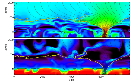
Figure 14: Vertical cross sections through the upper layers of a 3D MHD model by Wedemeyer-Böhm [206]. a) logarithmic magnetic field strength (color range 0.2 - 3.5 [G]), b) gas temperature (color range 2500 - 12000 K). The solid curves in both panels represent (projected) magnetic field lines (thin black curves), the contour for plasma-$\beta=1$ (thick yellow contour), and the height where the optical depth is unity (horizontally running black curve around $z=0$). The latter defines the bottom of the photosphere.

The chromospheric layer of the hydrodynamic CO5BOLD models by Wedemeyer et al. [92] exhibits a very dynamic and intermittent pattern made of propagating hot shock fronts and cool post-shock regions (cf. Fig. 14b). The resulting fluctuations of the gas properties are substantial like it was found already from 1D simulations. As the shock fronts are very narrow, the peak temperatures of 7000–8000 K in CO5BOLD simulations depend to some degree on the resolution of the computational grid. Adiabatic expansion of the post-shock regions produces gas temperatures down to $\sim 2000$ K. A similar shock pattern can already be perceived in the gas-temperature maps by Skartlien et al. [201] but much less clearly due to the lower spatial resolution. Martínez-Sykora et al. [64], who employed the Oslo Staggered Code for 3D simulations of magnetic-flux emergence, find a shock-induced pattern in their model chromosphere, too. The range in chromospheric gas temperature is similar to the CO5BOLD results, whereas there are differences in the temperature amplitudes. This is presumably caused by the different numerical treatment of the radiative transfer in the upper layers. The existence of a chromospheric small-scale pattern in quiet regions of the Sun is now supported by recent observations [e.g., 207, 208].

Also the MHD simulations carried out with CO5BOLD exhibit strong shock fronts in the chromosphere (see Fig. 14b). Compared to the photosphere below, the magnetic field in the model chromospheres is less concentrated and reaches a higher filling factor; it has a lower average field strength and evolves faster [53, 183]. See Sect. 4.4 for a description of the photosphere in this type of models. The topology of the chromospheric magnetic field is yet complex and features shock-induced compression and amplification into magnetic field filaments. Fig. 14a, shows the upper layers of a current 3D simulation. The vertical cross section is intersecting a magnetic flux concentration. The magnetic field lines (thin solid lines, projected into the view plane) show that the field is highly concentrated in the photosphere and expands in the chromosphere above. The thick yellow curve represents the surface where plasma-$\beta=1$. Although the height of this surface varies strongly, it is typically found around $z\sim 1000$ km outside strong magnetic flux concentrations. For plasma-$\beta=1$, sound speed and Alfvén speed are similar, which has important implications for the occurrence, conversion, and propagation of different wave modes [e.g., 209, 210, 211, 185, 187]. The simulations indeed show a different behavior in the domains with $\beta<1$ and $\beta>1$, resulting in a slowly evolving lower part and a highly dynamic upper part. Current sheets exist below and above the $\beta=1$ surface but differ in their orientation (see Fig. 13). They are stacked with predominantly horizontal orientation in the lower atmosphere (see Sect. 4.4) but are aligned with shock fronts in the low-$\beta$ regime in the chromosphere, resulting in oblique or even vertical orientation.

4.5.3 Next steps

The next steps towards realistic models of the solar chromosphere concern an improvement of the radiative transfer under chromospheric conditions and the detailed treatment of non-equilibrium processes that have a significant impact on the equation of state and the opacities. However, the detailed modeling of non-equilibrium effects might increase the computational costs to a degree that it can become impractical. For instance, important opacity sources that deviate from their equilibrium state can prevent the usage of numerically efficient opacity look-up tables (Sect. 3.6.2) and require a costly detailed line-by-line treatment of the radiation transfer. The inclusion of large-scale magnetic fields is another important point as most of the models discussed above resemble rather quiet Sun internetwork conditions with comparatively weak magnetic fields and thus cannot be applied to more active regions on the Sun. Chromospheric simulations with CO5BOLD have been restricted to heights below the transition region, where thermal conduction can still be neglected. Simulations that include the transition region and low corona have not been performed so far because it would require the implementation of the computationally expensive treatment of thermal conduction.

4.6 Local models of other stars

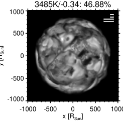
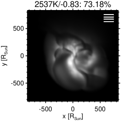
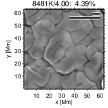
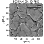
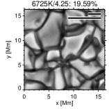
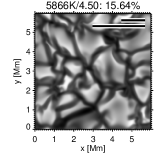
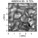
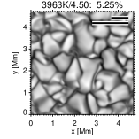
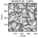
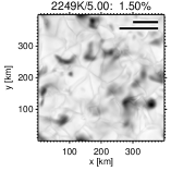
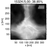
Figure 15: Frequency-integrated-intensity snapshots of global models of a red supergiant and an AGB star with low surface gravity (top row) and local models of stars near the main sequence with larger gravities. The title lines show the effective temperature, the decadic logarithm of the surface gravity in cm s², and the relative gray intensity contrast – averaged over a representative time span. The length of the upper bar in the top right of each frame is 10 times the surface pressure scale height. The bar below is 10 times the pressure scale height but measured 3 pressure scale heights below the other level.

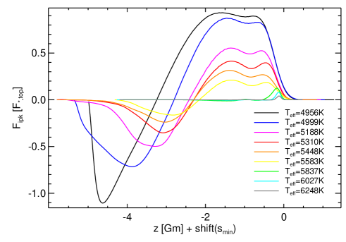
Figure 16: Convective fluxes (normalized by the flux emitted at the top of the model) versus height for a temperature sequence of cepheid models at $\log g$=2. The curves are shifted in $z$, so that the entropy minimum at the top of the convection zone lies at $z$=0.

Surface-intensity snapshots from the hot A-type star regime (about 8500 K) over solar-type stars ($T_{\mathrm{eff,Sun}}$=5775 K) to brown dwarfs (about 1500 K) are shown in Fig. 15. A-type stars [212, 213, 214] have only thin surface convection zones, where convection carries only a small fraction of the total energy flux. Of interest in these stars is the amount of overshoot below the convection zone, that causes a mixing of elements counteracting the separating effect of gravitational settling and radiative acceleration [36]. The shapes of spectral lines differ from solar counterparts [214], suggesting different atmospheric flow patterns or deviating correlations between temperature fluctuations and velocity fields. Due to the shorter radiative time scales, caused by efficient radiative energy exchange, the steeper and stronger subphotospheric temperature jump, and the larger convective cells, the simulations are numerically more challenging than those of solar-type stars, requiring more numerical grid cells and many more time steps. Therefore, the required CPU time per model goes up by a factor of 100 or more – depending on the stellar parameters – and an implicit treatment (at least of the radiation transport) seems appropriate [215]. The transition from a thin, inefficient convection zone to a deeper zone, where the convection carries in some layers almost all the energy flux, occurs in a similar way in the temperature sequence of 2D cepheid models at $\log g$=2 in Fig. 16. Remarkable is the extended overshoot region with significant negative convective flux.

F, G, and K dwarfs form a temperature sequence, in which the convection zone gets deeper, the Mach number of the convective velocity declines, the relative efficiency of convection compared to radiation increases, and the granular contrast decreases (Fig. 11). While the amplitude of pressure waves drops rapidly, the amplitude of gravity waves decreases more slowly: in solar models they are more difficult to detect than pressure waves [39], but they dominate in brown dwarfs [96] and influence the shape of the dust clouds (coolest models in Fig. 15). The change in the amount of photospheric overshoot and the optical depth at the top of the convection zone affect the appearance of granules in Fig. 15. The scale of the granules seems related to the surface – or rather the sub-surface – pressure scale height [216]. Both are indicated by the horizontal bars in Fig. 15, which have lengths of 10 $H_{p}$, measured at two different heights.

The first multi-D radiation-hydrodynamical model atmospheres for M-type stars were calculated by Ludwig and collaborators [217, 218] using the simulation code of Nordlund and Stein [219]. An important issue, that needed to be settled in the model construction, was the handling of molecular opacities in the opacity-binning scheme (see Sect. 3.6.2). It turned out that no particular treatment is necessary, as long as the molecular opacities dominate the atmospheric opacities. Subsequently, Wende et al. [157] used CO5BOLD with the previously developed opacity set-up to calculate a sequence of models covering the main-sequence in the temperature range $2600\,\mathrm{K}\leq T_{\mathrm{eff}}\leq 4000\,\mathrm{K}$, and probing surface gravities $3.0\leq\log(g)\leq 5.0$ at fixed effective temperature of $\approx 3300\,\mathrm{K}$. Motivated by observational demands, the authors investigated the impact of the velocity field and thermal structure on properties of FeH lines.

While the 2616 K model of an M-dwarf in Fig. 15 does not show visible amounts of dust, in brown dwarfs at even lower temperatures, dust clouds begin to form in the atmospheres [96], that show up as small dark patches (shaped by gravity waves) above the low-contrast granules in the 2249 K model in Fig. 15. The coolest model in Fig. 15 has completely opaque dust clouds, that hide the underlying gas convection zone. A long-wavelength and high-amplitude gravity wave creates the large-scale pattern in the plot, while convection within the dust clouds causes the thin bright filaments. The numerical challenges in these simulations come from the – hardly known – non-equilibrium dust chemistry, the long relaxation times of dust settling and mixing, and the need to account for the likely interaction of small “cloud” scales, covered by the local models in Freytag et al. [96], and global “weather front” scales, far beyond the size of the computational domain of the local models.

Cool hydrogen-rich white dwarfs are old stars, that have used up their nuclear fuel and cool down slowly. The large surface gravity causes high atmospheric pressures, small convective scales, and a settling of elements heavier than hydrogen from the atmosphere into subsurface layers. Recently, first models for those objects were computed with CO5BOLD [220]. The work follows up on earlier investigations by some of the authors (HGL, BF, MS) and collaborators [109, 221, 222] using a code which was a precursor of CO5BOLD. Similar to the case of M-type models, the intention is to study the influence of multi-D effects on the formation of Balmer lines.

4.7 Global models of supergiants and AGB stars

Early explanations of the irregular light curves of red supergiants as due to giant convection cells by Stothers and Leung [223] and Schwarzschild [224] got more recently support by interferometric detections of spatial inhomogeneities on the surface of Betelgeuse (e.g., [225]). When convective scales are not very small compared to the stellar diameter, global star-in-a-box simulations are possible (Sect. 3.2.2) making these stars the easiest targets for global models, that include a major part of the convective envelope as well as the near environment of the star. The top row of Fig. 15 shows snapshots of the emergent intensity of such models: on the left from a red-supergiant [158] and on the right from an AGB-star simulation [144]. The supergiant model confirms that convective scales are indeed huge, with a few very large, deep, long-lived envelope cells and many small, short-lived surface cells. The surface contrast is enormous (see Fig. 11), due to violent convective flows and in addition waves, that have already in the lower photosphere a large amplitude, in contrast to the solar case. Large scales and contrast values render the features observable with current interferometers: the models compare favorably with VLTI observations [159, 226, 160] indicating that these global models start to become “realistic”, too.

RHD simulations of an AGB star (Fig. 15, top right [144]) demonstrate that convection can excite pressure waves with amplitudes sufficient to turn them into shocks, which then push out dense material into layers cool enough that dust can form (included in the 3D models, see Sect. 3.8.3). This allows radiation pressure on dust to accelerate the material outward causing a stellar wind (not included yet in the 3D models of Freytag and Höfner [144] but in the 1D simulations of Höfner et al. [106, 107]). Major challenges for the simulations are posed by the molecular opacities varying strongly with frequency, that cause – together with large dust opacities – very small radiative time steps during the time-explicit treatment of the radiative energy exchange. So far, only 1D RHD models (e.g., [107]) include important ingredients like scattering, radiation pressure, and a sufficiently large computational volume to account for the extended wind acceleration region. While the properties of the simulated surface granulation seem already quite realistic, there are discrepancies further out: The models have a too steep density drop and show no “molsphere”, chromosphere, or wind. Future generations of models will help to investigate the role of radiation pressure on molecular lines and dust, magnetic fields, and rotation for these outer layers.

5 Conclusions

For stellar parameters close to the solar values, the transition from 1D static stellar-atmosphere models to 3D dynamic local stellar-atmosphere simulations is in full swing. RHD simulations of surface convection of such stars are routinely performed by codes like CO5BOLD, as presented in this paper. There is a good consistency between the results of similar codes and with solar observations. The simulations provide insight into processes related to stellar surface convection, and deliver high-accuracy model atmospheres for spectrum-synthesis and abundance-determination work for a variety of stellar parameters.

However, many physical effects are not properly incorporated by the current models: small-scale convective structures, covered by local-box simulations, interact with their environment via, for instance, large-scale convective flows, magnetic fields, waves, or global dust flows (the latter in cool substellar objects). The inclusion of the chromosphere, the corona, the wind-formation zone, etc., requires to cover an even wider range of densities and temperatures than the previous models. At lower densities, the detailed treatment of non-equilibrium processes (molecule formation, radiation transport not in local thermal equilibrium) are a major challenge, requiring algorithms with a complexity far beyond the current treatment. The modeling of magnetic phenomena needs appropriate MHD or plasma-physics simulations. Objects significantly cooler than the Sun require a detailed non-equilibrium treatment of dust and “weather phenomena”. Varying efficiency ratios between radiation and convection as a function of stellar parameters have to be considered: the extremely small radiative relaxation time scale in hotter stars causes small numerical time steps and slows down simulations significantly. Cool objects on the other hand need extended simulation runs because of their long thermal relaxation time scales. Low-gravity objects have extended atmospheres and can produce winds. Magnetic-field phenomena exist on very large and very small scales and couple the stellar interior to the photosphere and the envelope. In stars more active than the Sun, the fields are stronger and can form very different configurations.

In the future, we will see a refinement of local simulations and more and more extended model grids, providing reliable stellar model atmospheres. However, the main challenges arise from the need to extend the simulations in terms of stellar parameters (from A-type stars to planetary objects and from supergiants to white dwarfs), from physical effects, and from the extension of spatial and temporal scales towards 3D large-scale or even global dynamic models. These models should not only include the photosphere but the stellar interior and the outer atmospheric layers as well, covering short and long time scales (many rotation periods, dynamo cycles, stellar oscillation periods, climate cycles).

Realistic global 3D MHD simulations for cool stars will remain a dream for the foreseeable future. Nevertheless, numerical simulations will continue to be indispensable tools for the understanding of the various complex dynamical processes in stars.

References

- Vitense [1953] E. Vitense, Die Wasserstoffkonvektionszone der Sonne, Zeitschrift für Astrophysik 32 (1953) 135–164.
- Böhm-Vitense [1958] E. Böhm-Vitense, Über die Wasserstoffkonvektionszone in Sternen verschiedener Effektivtemperaturen und Leuchtkräfte, Zeitschrift für Astrophysik 46 (1958) 108–143.
- Mihalas [1978] D. Mihalas, Stellar atmospheres, W. H. Freeman and Co., San Francisco, 2nd edition, 1978.
- Kurucz [1970] R. L. Kurucz, Atlas: a Computer Program for Calculating Model Stellar Atmospheres, SAO Special Report 309 (1970).
- Kurucz [2005] R. L. Kurucz, ATLAS12, SYNTHE, ATLAS9, WIDTH9, et cetera, Mem. Soc. Astron. Italiana Suppl. 8 (2005) 14–24.
- Gustafsson et al. [1975] B. Gustafsson, R. A. Bell, K. Eriksson, Å. Nordlund, A grid of model atmospheres for metal-deficient giant stars. I, A&A 42 (1975) 407–432.
- Gustafsson et al. [2008] B. Gustafsson, B. Edvardsson, K. Eriksson, U. G. Jørgensen, Å. Nordlund, B. Plez, A grid of MARCS model atmospheres for late-type stars. I. Methods and general properties, A&A 486 (2008) 951–970.
- Allard and Hauschildt [1995] F. Allard, P. H. Hauschildt, Model atmospheres for M (sub)dwarf stars. I. The base model grid, ApJ 445 (1995) 433–450.
- Allard et al. [2001] F. Allard, P. H. Hauschildt, D. R. Alexander, A. Tamanai, A. Schweitzer, The Limiting Effects of Dust in Brown Dwarf Model Atmospheres, ApJ 556 (2001) 357–372.
- Steffen and Jordan [2000] M. Steffen, S. Jordan, Numerical Simulation of Stellar Convection: Comparison with Mixing-length Theory, in: P. Murdin (Ed.), Encyclopedia of Astronomy and Astrophysics, Taylor and Francis Group, 2000.
- Fuhrmann et al. [1993] K. Fuhrmann, M. Axer, T. Gehren, Balmer lines in cool dwarf stars. I. Basic influence of atmospheric models, A&A 271 (1993) 451–462.
- Steffen and Ludwig [1999] M. Steffen, H. Ludwig, Balmer Line Formation in Convective Stellar Atmospheres, in: A. Gimenez, E. F. Guinan, B. Montesinos (Eds.), Stellar Structure: Theory and Test of Convective Energy Transport, volume 173 of Astronomical Society of the Pacific Conference Series, pp. 217–220.
- Christensen-Dalsgaard et al. [1996] J. Christensen-Dalsgaard, W. Däppen, S. V. Ajukov, E. R. Anderson, H. M. Antia, S. Basu, V. A. Baturin, G. Berthomieu, B. Chaboyer, S. M. Chitre, A. N. Cox, P. Demarque, J. Donatowicz, W. A. Dziembowski, M. Gabriel, D. O. Gough, D. B. Guenther, J. A. Guzik, J. W. Harvey, F. Hill, G. Houdek, C. A. Iglesias, A. G. Kosovichev, J. W. Leibacher, P. Morel, C. R. Proffitt, J. Provost, J. Reiter, E. J. Rhodes, Jr., F. J. Rogers, I. W. Roxburgh, M. J. Thompson, R. K. Ulrich, The Current State of Solar Modeling, Science 272 (1996) 1286–1292.
- Bahcall et al. [2001] J. N. Bahcall, M. H. Pinsonneault, S. Basu, Solar Models: Current Epoch and Time Dependences, Neutrinos, and Helioseismological Properties, ApJ 555 (2001) 990–1012.
- Latour et al. [1976] J. Latour, E. A. Spiegel, J. Toomre, J. Zahn, Stellar convection theory. I. The anelastic modal equations, ApJ 207 (1976) 233–243.
- Latour et al. [1981] J. Latour, J. Toomre, J. Zahn, Stellar convection theory. III. Dynamical coupling of the two convection zones in A-type stars by penetrative motions, ApJ 248 (1981) 1081–1098.
- Toomre et al. [1976] J. Toomre, J. Zahn, J. Latour, E. A. Spiegel, Stellar convection theory. II. Single-mode study of the second convection zone in an A-type star, ApJ 207 (1976) 545–563.
- Musman and Nelson [1976] S. Musman, G. D. Nelson, The energy balance of granulation, ApJ 207 (1976) 981–988.
- Nelson [1978] G. D. Nelson, A two-dimensional solar model, Solar Physics 60 (1978) 5–18.
- Chan and Wolff [1982] K. L. Chan, C. L. Wolff, ADI on staggered mesh—A method for calculation of compressible convection, J. Comput. Phys. 451 (1982) 109–129.
- Hurlburt et al. [1984] N. E. Hurlburt, J. Toomre, J. M. Massaguer, Two-dimensional compressible convection extending over multiple scale heights, ApJ 282 (1984) 557–573.
- Steffen et al. [1989] M. Steffen, H.-G. Ludwig, A. Krüß, A numerical simulation study of solar granular convection in cells of different horizontal dimension, A&A 213 (1989) 371–382.
- Nordlund [1982] Å. Nordlund, Numerical simulations of the solar granulation. I. Basic equations and methods, A&A 107 (1982) 1–10.
- Dravins et al. [1981] D. Dravins, L. Lindegren, Å. Nordlund, Solar granulation - Influence of convection on spectral line asymmetries and wavelength shifts, A&A 96 (1981) 345–364.
- Toomre et al. [1990] J. Toomre, N. Brummell, F. Cattaneo, N. E. Hurlburt, Three-dimensional compressible convection at low Prandtl numbers, Computer Physics Communications 59 (1990) 105–117.
- Malagoli et al. [1990] A. Malagoli, F. Cattaneo, N. H. Brummell, Turbulent supersonic convection in three dimensions, ApJL 361 (1990) L33–L36.
- Cattaneo et al. [1991] F. Cattaneo, N. H. Brummell, J. Toomre, A. Malagoli, N. E. Hurlburt, Turbulent compressible convection, ApJ 370 (1991) 282–294.
- Hossain and Mullan [1991] M. Hossain, D. J. Mullan, Three-dimensional compressible hydrodynamic convection in the Sun and stars, ApJ 380 (1991) 631–654.
- Singh and Chan [1993] H. P. Singh, K. L. Chan, A study of the three-dimensional turbulent compressible convection in a deep atmosphere at various Prandtl numbers, A&A 279 (1993) 107–118.
- Asplund [2005] M. Asplund, New Light on Stellar Abundance Analyses: Departures from LTE and Homogeneity, Ann. Rev. Astron. & Astrophys. 43 (2005) 481–530.
- Asplund et al. [2009] M. Asplund, N. Grevesse, A. J. Sauval, P. Scott, The Chemical Composition of the Sun, Ann. Rev. Astron. & Astrophys. 47 (2009) 481–522.
- Caffau et al. [2008] E. Caffau, H.-G. Ludwig, M. Steffen, T. R. Ayres, P. Bonifacio, R. Cayrel, B. Freytag, B. Plez, The photospheric solar oxygen project. I. Abundance analysis of atomic lines and influence of atmospheric models, A&A 488 (2008) 1031–1046.
- Caffau et al. [2011] E. Caffau, H.-G. Ludwig, M. Steffen, B. Freytag, P. Bonifacio, Solar Chemical Abundances Determined with a CO5BOLD 3D Model Atmosphere, Solar Physics (2011) 255–269.
- Cayrel et al. [2007] R. Cayrel, M. Steffen, H. Chand, P. Bonifacio, M. Spite, F. Spite, P. Petitjean, H.-G. Ludwig, E. Caffau, Line shift, line asymmetry, and the 6Li/7Li isotopic ratio determination, A&A 473 (2007) L37–L40.
- Ludwig et al. [1999] H.-G. Ludwig, B. Freytag, M. Steffen, A calibration of the mixing-length for solar-type stars based on hydrodynamical simulations. I. Methodical aspects and results for solar metallicity, A&A 346 (1999) 111–124.
- Freytag et al. [1996] B. Freytag, H.-G. Ludwig, M. Steffen, Hydrodynamical models of stellar convection. The role of overshoot in DA white dwarfs, A-type stars, and the Sun, A&A 313 (1996) 497–516.
- Samadi et al. [2003] R. Samadi, Å. Nordlund, R. F. Stein, M. J. Goupil, I. Roxburgh, Numerical 3D constraints on convective eddy time-correlations: Consequences for stochastic excitation of solar p modes, A&A 404 (2003) 1129–1137.
- Samadi et al. [2007] R. Samadi, D. Georgobiani, R. Trampedach, M. J. Goupil, R. F. Stein, Å. Nordlund, Excitation of solar-like oscillations across the HR diagram, A&A 463 (2007) 297–308.
- Straus et al. [2008] T. Straus, B. Fleck, S. M. Jefferies, G. Cauzzi, S. W. McIntosh, K. Reardon, G. Severino, M. Steffen, The Energy Flux of Internal Gravity Waves in the Lower Solar Atmosphere, ApJL 681 (2008) L125–L128.
- Grossmann-Doerth et al. [1989] U. Grossmann-Doerth, M. Knölker, M. Schüssler, E. Weisshaar, Models of Magnetic Flux Sheets, in: R. J. Rutten, G. Severino (Eds.), Solar and Stellar Granulation, volume 263 of NATO Advanced Science Institutes, Series C, Kluwer Acad. Publishers, Dordrecht, 1989, pp. 481–492.
- Steiner et al. [1998] O. Steiner, U. Grossmann-Doerth, M. Knölker, M. Schüssler, Dynamical Interaction of Solar Magnetic Elements and Granular Convection: Results of a Numerical Simulation, ApJ 495 (1998) 468–484.
- Steiner et al. [1994] O. Steiner, M. Knölker, M. Schüssler, Dynamic interaction of convection with magnetic flux sheets: First results of a new MHD code, in: R. J. Rutten, C. J. Schrijver (Eds.), Solar Surface Magnetism, Kluwer Academic Publishers, Dordrecht, 1994, pp. 441–470.
- Atroshchenko and Sheminova [1996] I. N. Atroshchenko, V. A. Sheminova, Numerical simulation of the interaction between solar granules and small-scale magnetic fields., Kinematics and Physics of Celestial Bodies 12 (1996) 21–32.
- Nordlund [1986] Å. Nordlund, 3-D Model Calculations, in: W. Deinzer, M. Knölker, H. H. Voigt (Eds.), Small Scale Magnetic Flux Concentrations in the Solar Photosphere, Vandenhoeck & Ruprecht, Göttingen, 1986, pp. 83–102.
- Nordlund et al. [2009] Å. Nordlund, R. F. Stein, M. Asplund, Solar Surface Convection, Living Reviews in Solar Physics 6 (2009) 2.
- Galloway and Weiss [1981] D. J. Galloway, N. O. Weiss, Convection and magnetic fields in stars, ApJ 243 (1981) 945–953.
- Deinzer et al. [1984] W. Deinzer, G. Hensler, M. Schüssler, E. Weisshaar, Model calculations of magnetic flux tubes. II. Stationary results for solar magnetic elements, A&A 139 (1984) 426–449.
- Hurlburt and Toomre [1988] N. E. Hurlburt, J. Toomre, Magnetic fields interacting with nonlinear compressible convection, ApJ 327 (1988) 920–932.
- Weiss et al. [1990] N. O. Weiss, D. P. Brownjohn, N. E. Hurlburt, M. R. E. Proctor, Oscillatory convection in sunspot umbrae, MNRAS 245 (1990) 434–452.
- Fox et al. [1991] P. A. Fox, M. L. Theobald, S. Sofia, Compressible magnetic convection - Formulation and two-dimensional models, ApJ 383 (1991) 860–881.
- Hansteen and Gudiksen [2005] V. H. Hansteen, B. Gudiksen, 3D Numerical Models of Quiet Sun Coronal Heating, in: B. Fleck, T. H. Zurbuchen, H. Lacoste (Eds.), Connecting Sun and Heliosphere, volume 592 of ESA Special Publication, pp. 483–486.
- Gudiksen et al. [2011] B. V. Gudiksen, M. Carlsson, V. H. Hansteen, W. Hayek, J. Leenaarts, J. Martínez-Sykora, The stellar atmosphere simulation code Bifrost. Code description and validation, A&A 531 (2011) A154.
- Schaffenberger et al. [2005] W. Schaffenberger, S. Wedemeyer-Böhm, O. Steiner, B. Freytag, Magnetohydrodynamic Simulation from the Convection Zone to the Chromosphere, in: D. E. Innes, A. Lagg, S. A. Solanki (Eds.), Chromospheric and Coronal Magnetic Fields, volume 596 of ESA Special Publication, p. 65.
- Vögler et al. [2005] A. Vögler, S. Shelyag, M. Schüssler, F. Cattaneo, T. Emonet, T. Linde, Simulations of magneto-convection in the solar photosphere. Equations, methods, and results of the MURaM code, A&A 429 (2005) 335–351.
- Heinemann et al. [2007] T. Heinemann, Å. Nordlund, G. B. Scharmer, H. C. Spruit, MHD Simulations of Penumbra Fine Structure, ApJ 669 (2007) 1390–1394.
- Jacoutot et al. [2008] L. Jacoutot, A. G. Kosovichev, A. Wray, N. N. Mansour, Realistic Numerical Simulations of Solar Convection and Oscillations in Magnetic Regions, ApJL 684 (2008) L51–L54.
- Muthsam et al. [2010] H. J. Muthsam, F. Kupka, B. Löw-Baselli, C. Obertscheider, M. Langer, P. Lenz, ANTARES - A Numerical Tool for Astrophysical RESearch with applications to solar granulation, New Astronomy 15 (2010) 460–475.
- Stein et al. [2009] R. F. Stein, Å. Nordlund, D. Georgoviani, D. Benson, W. Schaffenberger, Supergranulation-Scale Convection Simulations, in: M. Dikpati, T. Arentoft, I. González Hernández, C. Lindsey, F. Hill (Eds.), Solar-Stellar Dynamos as Revealed by Helio- and Asteroseismology, volume 416 of Astronomical Society of the Pacific Conference Series, pp. 421–426.
- Nordlund and Galsgaard [1995] Å. Nordlund, K. Galsgaard, A 3D MHD code for Parallel Computers, Tech. Rep., Astron. Observ., Copenhagen Univ. (1995).
- Cheung et al. [2010] M. C. M. Cheung, M. Rempel, A. M. Title, M. Schüssler, Simulation of the Formation of a Solar Active Region, ApJ 720 (2010) 233–244.
- Rempel et al. [2009] M. Rempel, M. Schüssler, R. H. Cameron, M. Knölker, Penumbral Structure and Outflows in Simulated Sunspots, Science 325 (2009) 171–174.
- Hansteen et al. [2007] V. H. Hansteen, M. Carlsson, B. Gudiksen, 3D Numerical Models of the Chromosphere, Transition Region, and Corona, in: P. Heinzel, I. Dorotovič, R. J. Rutten (Eds.), The Physics of Chromospheric Plasmas, volume 368 of Astronomical Society of the Pacific Conference Series, pp. 107–114.
- Hansteen et al. [2010] V. H. Hansteen, H. Hara, B. De Pontieu, M. Carlsson, On Redshifts and Blueshifts in the Transition Region and Corona, ApJ 718 (2010) 1070–1078.
- Martínez-Sykora et al. [2008] J. Martínez-Sykora, V. Hansteen, M. Carlsson, Twisted Flux Tube Emergence From the Convection Zone to the Corona, ApJ 679 (2008) 871–888.
- Abbett [2007] W. P. Abbett, The Magnetic Connection between the Convection Zone and Corona in the Quiet Sun, ApJ 665 (2007) 1469–1488.
- Abbett and Fisher [2010] W. P. Abbett, G. H. Fisher, Improving large-scale convection-zone-to-corona models, Mem. Soc. Astron. Italiana 81 (2010) 721–728.
- Isobe et al. [2008] H. Isobe, M. R. E. Proctor, N. O. Weiss, Convection-driven Emergence of Small-Scale Magnetic Fields and their Role in Coronal Heating and Solar Wind Acceleration, ApJL 679 (2008) L57–L60.
- Weiss et al. [1996] N. O. Weiss, D. P. Brownjohn, P. C. Matthews, M. R. E. Proctor, Photospheric Convection in Strong Magnetic Fields, MNRAS 283 (1996) 1153–1164.
- Tobias et al. [1998] S. M. Tobias, N. H. Brummell, T. L. Clune, J. Toomre, Pumping of Magnetic Fields by Turbulent Penetrative Convection, ApJL 502 (1998) L177–L180.
- Cattaneo [1999] F. Cattaneo, On the Origin of Magnetic Fields in the Quiet Photosphere, ApJL 515 (1999) L39–L42.
- Ossendrijver et al. [2001] M. Ossendrijver, M. Stix, A. Brandenburg, Magnetoconvection and dynamo coefficients: Dependence of the alpha effect on rotation and magnetic field, A&A 376 (2001) 713–726.
- Cattaneo et al. [2003] F. Cattaneo, T. Emonet, N. Weiss, On the Interaction between Convection and Magnetic Fields, ApJ 588 (2003) 1183–1198.
- Archontis et al. [2005] V. Archontis, F. Moreno-Insertis, K. Galsgaard, A. W. Hood, The Three-dimensional Interaction between Emerging Magnetic Flux and a Large-Scale Coronal Field: Reconnection, Current Sheets, and Jets, ApJ 635 (2005) 1299–1318.
- Cheung et al. [2006] M. C. M. Cheung, F. Moreno-Insertis, M. Schüssler, Moving magnetic tubes: fragmentation, vortex streets and the limit of the approximation of thin flux tubes, A&A 451 (2006) 303–317.
- Glatzmaier [1984] G. A. Glatzmaier, Numerical simulations of stellar convective dynamos. I. The model and method, J. Comput. Phys. 55 (1984) 461–484.
- Browning et al. [2006] M. K. Browning, M. S. Miesch, A. S. Brun, J. Toomre, Dynamo Action in the Solar Convection Zone and Tachocline: Pumping and Organization of Toroidal Fields, ApJL 648 (2006) L157–L160.
- Clune et al. [1999] T. C. Clune, J. R. Elliott, M. S. Miesch, J. Toomre, G. A. Glatzmaier, Computational aspects of a code to study rotating turbulent convection in spherical shells, Parallel Computing 588 (1999) 361–380.
- Dobler et al. [2006] W. Dobler, M. Stix, A. Brandenburg, Magnetic Field Generation in Fully Convective Rotating Spheres, ApJ 638 (2006) 336–347.
- Ziegler [2005] U. Ziegler, Self-gravitational adaptive mesh magnetohydrodynamics with the NIRVANA code, A&A 435 (2005) 385–395.
- Nordlund and Stein [2009] Å. Nordlund, R. F. Stein, Accurate Radiation Hydrodynamics and MHD Modeling of 3-D Stellar Atmospheres, in: I. Hubeny, J. M. Stone, K. MacGregor, K. Werner (Eds.), Recent Directions in Astrophysical Quantitative Spectroscopy and Radiation Hydrodynamics, volume 1171 of American Institute of Physics Conference Series, pp. 242–259.
- Carlsson [2009] M. Carlsson, Hydrodynamics and radiative transfer of 3D model atmospheres. Current status, limitations, and how to make headway, Mem. Soc. Astron. Italiana 80 (2009) 606–613.
- Steiner [2010] O. Steiner, Magnetic Coupling in the Quiet Solar Atmosphere, in: S. S. Hasan, R. J. Rutten (Eds.), Magnetic Coupling between the Interior and Atmosphere of the Sun, Springer, 2010, pp. 166–185.
- Spitzer [1962] L. Spitzer, Physics of Fully Ionized Gases, Interscience Publishers, New York, 2nd edition, 1962.
- Thomas [1930] L. H. Thomas, The radiation field in a fluid in motion, The Quarterly Journal of Mathematics 1 (1930) 239–251.
- Nordlund et al. [1997] Å. Nordlund, H. C. Spruit, H.-G. Ludwig, R. Trampedach, Is stellar granulation turbulence?, A&A 328 (1997) 229–234.
- Spiegel [1957] E. A. Spiegel, The Smoothing of Temperature Fluctuations by Radiative Transfer, ApJ 126 (1957) 202–207.
- Unno and Spiegel [1966] W. Unno, E. A. Spiegel, The Eddington Approximation in the Radiative Heat Equation, Publ. Astron. Soc. Japan 18 (1966) 85–95.
- Brun et al. [2004] A. S. Brun, M. S. Miesch, J. Toomre, Global-Scale Turbulent Convection and Magnetic Dynamo Action in the Solar Envelope, ApJ 614 (2004) 1073–1098.
- Schrijver [2001] C. J. Schrijver, Catastrophic cooling and high-speed downflow in quiescent solar coronal loops observed with TRACE, Solar Physics 198 (2001) 325–345.
- Klimchuk [2006] J. A. Klimchuk, On Solving the Coronal Heating Problem, Solar Physics 234 (2006) 41–77.
- Strang [1968] G. Strang, On the construction and comparison of difference schemes, SIAM J. Numer. Anal. 5 (1968) 506–517.
- Wedemeyer et al. [2004] S. Wedemeyer, B. Freytag, M. Steffen, H.-G. Ludwig, H. Holweger, Numerical simulation of the three-dimensional structure and dynamics of the non-magnetic solar chromosphere, A&A 414 (2004) 1121–1137.
- Iglesias et al. [1992] C. A. Iglesias, F. J. Rogers, B. G. Wilson, Spin-orbit interaction effects on the Rosseland mean opacity, ApJ 397 (1992) 717–728.
- Hauschildt et al. [1997] P. H. Hauschildt, E. Baron, F. Allard, Parallel Implementation of the PHOENIX Generalized Stellar Atmosphere Program, ApJ 483 (1997) 390–398.
- Steffen and Freytag [1995] M. Steffen, B. Freytag, Lyapunov exponents for solar surface convection, Chaos Solitons and Fractals 5 (1995) 1965–1973.
- Freytag et al. [2010] B. Freytag, F. Allard, H.-G. Ludwig, D. Homeier, M. Steffen, The role of convection, overshoot, and gravity waves for the transport of dust in M dwarf and brown dwarf atmospheres, A&A 513 (2010) A19.
- Roe [1986] P. Roe, Characteristic-Based Schemes for the Euler Equations, Ann. Rev. Fluid Mech. 18 (1986) 337.
- LeVeque [1992] R. J. LeVeque, Numerical Methods for Conservation Laws, Birkhäuser Verlag, Basel, 1992.
- Colella and Woodward [1984] P. Colella, P. R. Woodward, The Piecewise Parabolic Method (PPM) for Gas-Dynamical Simulations, J. Comput. Phys. 54 (1984) 174–201.
- Mellema et al. [1991] G. Mellema, F. Eulderink, V. Icke, Hydrodynamical models of aspherical planetary nebulae, A&A 252 (1991) 718–732.
- Mottura et al. [1997] L. Mottura, L. Vigevano, M. Zaccanti, An Evaluation of Roe’s Scheme Generalizations for Equilibrium Real Gas Flows, J. Comput. Phys. 138 (1997) 354–399.
- Glaister [1988] P. Glaister, An approximate linearized Riemann solver for the Euler equations for real gases,, J. Comput. Phys. 74 (1988) 382–408.
- Quirk [1994] J. Quirk, A contribution to the great Riemann solver debate, Int. J. for Numerical Methods in Fluids 18 (1994) 555–574.
- Smagorinsky [1963] J. S. Smagorinsky, General Circulation experiments with the primitive equations I. The basic experiment, Monthly Weather Rev. 91 (1963) 99–164.
- Stone et al. [1992] J. M. Stone, D. Mihalas, M. L. Norman, ZEUS-2D: A radiation magnetohydrodynamics code for astrophysical flows in two space dimensions. III. The radiation hydrodynamic algorithms and tests, ApJS 80 (1992) 819–845.
- Höfner et al. [1995] S. Höfner, M. U. Feuchtinger, E. A. Dorfi, Dust formation in winds of long-period variables. III. Dynamical models and confirmation of a dust-induced -mechanism, A&A 297 (1995) 815–827.
- Höfner et al. [2003] S. Höfner, R. Gautschy-Loidl, B. Aringer, U. G. Jørgensen, Dynamic model atmospheres of AGB stars. III. Effects of frequency-dependent radiative transfer, A&A 399 (2003) 589–601.
- Ludwig [1992] H.-G. Ludwig, Non-gray radiation transport in numerical simulations of stellar convection, Ph.D. thesis, University of Kiel, 1992.
- Ludwig et al. [1994] H.-G. Ludwig, S. Jordan, M. Steffen, Numerical simulations of convection at the surface of a ZZ Ceti white dwarf, A&A 284 (1994) 105–117.
- Vögler [2004] A. Vögler, Effects of non-grey radiative transfer on 3D simulations of solar magneto-convection, A&A 421 (2004) 755–762.
- Davis and Polonsky [1972] P. J. Davis, I. Polonsky, Numerical Interpolation, Differentiation and Integration, in: M. Abramowitz, I. A. Stegun (Eds.), Handbook of Mathematical Functions, Dover Publications, New York, 1972, pp. 877–924.
- Steffen [1990] M. Steffen, A Simple Method for Monotonic Interpolation in One Dimension, A&A 239 (1990) 443–450.
- Feautrier [1964] P. Feautrier, Sur la résolution numérique de l’équation de transfert, Comptes Rendus de l’Académie des Sciences 258 (1964) 3189–3194.
- Cannon [1970] C. J. Cannon, Line Transfer in Two Dimensions, ApJ 161 (1970) 255–264.
- Avrett and Loeser [1971] E. H. Avrett, R. Loeser, Radiative transfer in two-component stellar atmospheres, J. Quant. Spectrosc. & Rad. Transfer 11 (1971) 559–571.
- Jones and Skumanich [1973] H. P. Jones, A. Skumanich, The Formation of Resonance Lines in Multidimensional Media. II. Radiation Operators and Their Numerical Representation, ApJ 185 (1973) 167–182.
- Jones [1973] H. P. Jones, The Formation of Resonance Lines in Multidimensional Media. III. Interpolation Functions, Accuracy, and Stability, ApJ 185 (1973) 183–196.
- Mihalas et al. [1978] D. Mihalas, L. H. Auer, B. R. Mihalas, Two-dimensional radiative transfer. I. Planar geometry, ApJ 220 (1978) 1001–1023.
- Kunasz and Auer [1988] P. Kunasz, L. H. Auer, Short characteristic integration of radiative transfer problems - Formal solution in two-dimensional slabs, J. Quant. Spectrosc. & Rad. Transfer 39 (1988) 67–79.
- Brackbill and Barnes [1980] J. U. Brackbill, D. C. Barnes, The effect of nonzero product of magnetic gradient and B on the numerical solution of the magnetohydrodynamic equations, J. Comput. Phys. 35 (1980) 426–430.
- Gombosi et al. [1994] T. I. Gombosi, K. G. Powell, D. L. de Zeeuw, Axisymmetric modeling of cometary mass loading on an adaptively refined grid: MHD results, J. Geopys. Res. 99 (1994) 21525–21539.
- Powell [1994] K. G. Powell, An approximate Riemann solver for magnetohydrodynamics (that works in more than one dimension), Technical Report ICASE-Report 94-24 (NASA CR-194902), NASA Langley Research Center, Hampton, VA 23681-0001, 1994.
- Evans and Hawley [1988] C. R. Evans, J. F. Hawley, Simulation of magnetohydrodynamic flows - A constrained transport method, ApJ 332 (1988) 659–677.
- Tóth [2000] G. Tóth, The Constraint in Shock-Capturing Magnetohydrodynamics Codes, J. Comput. Phys. 161 (2000) 605–652.
- Balsara and Spicer [1999] D. S. Balsara, D. Spicer, Maintaining Pressure Positivity in Magnetohydrodynamic Simulations, J. Comput. Phys. 148 (1999) 133–148.
- Janhunen [2000] P. Janhunen, A Positive Conservative Method for Magnetohydrodynamics Based on HLL and Roe Methods, J. Comput. Phys. 160 (2000) 649–661.
- van Leer [1984] B. van Leer, On the Relation between the Upwind-Differencing Schemes of Godunov, Enquist-Osher and Roe, SIAM J. Sci. Stat. Comput. 5 (1984) 1–20.
- Toro [2009] E. F. Toro, Riemann Solvers and Numerical Methods for Fluid Dynamics, A Practical Introduction, Springer, 3rd edition, 2009.
- Gottlieb and Shu [1998] S. Gottlieb, C. W. Shu, Total variation diminishing Runge-Kutta schemes, Mathematics of Computation 67 (1998) 73–85.
- Harten et al. [1983] A. Harten, P. D. Lax, B. van Leer, On Upstream Differencing and Godunov-Type Schemes for Hyperbolic Conservation Laws, SIAM Review 25 (1983) 35–61.
- Einfeldt et al. [1991] B. Einfeldt, P. L. Roe, C. D. Munz, B. Sjogreen, On Godunov-type methods near low densities, J. Comput. Phys. 92 (1991) 273–295.
- Balsara and Spicer [1999] D. S. Balsara, D. S. Spicer, A Staggered Mesh Algorithm Using High Order Godunov Fluxes to Ensure Solenoidal Magnetic Fields in Magnetohydrodynamic Simulations, J. Comput. Phys. 149 (1999) 270–292.
- Rempel et al. [2009] M. Rempel, M. Schüssler, M. Knölker, Radiative Magnetohydrodynamic Simulation of Sunspot Structure, ApJ 691 (2009) 640–649.
- Stone and Pringle [2001] J. M. Stone, J. E. Pringle, Magnetohydrodynamical non-radiative accretion flows in two dimensions, MNRAS 322 (2001) 461–472.
- Wedemeyer-Böhm et al. [2005] S. Wedemeyer-Böhm, I. Kamp, J. Bruls, B. Freytag, Carbon monoxide in the solar atmosphere. I. Numerical method and two-dimensional models, A&A 438 (2005) 1043–1057.
- Brown et al. [1989] P. Brown, G. Byrne, A. Hindmarsh, VODE: A Variable-Coefficient ODE Solver, SIAM J. Sci. Stat. Comp. 10 (1989) 1038–1051.
- Wedemeyer-Böhm and Steffen [2007] S. Wedemeyer-Böhm, M. Steffen, Carbon monoxide in the solar atmosphere. II. Radiative cooling by CO lines, A&A 462 (2007) L31–L35.
- Steffen and Muchmore [1988] M. Steffen, D. Muchmore, Can granular fluctuations in the solar photosphere produce temperature inhomogeneities at the height of the temperature minimum?, A&A 193 (1988) 281–290.
- Sollum [1999] E. Sollum, Hydrogen Ionization in the Solar Atmosphere: Exact and Simplified Treatments, Master’s thesis, University of Oslo, 1999.
- Carlsson and Stein [2002] M. Carlsson, R. F. Stein, Dynamic Hydrogen Ionization, ApJ 572 (2002) 626–635.
- Leenaarts and Wedemeyer-Böhm [2006] J. Leenaarts, S. Wedemeyer-Böhm, Time-dependent hydrogen ionisation in 3D simulations of the solar chromosphere. Methods and first results, A&A 460 (2006) 301–307.
- Helling et al. [2001] C. Helling, M. Oevermann, M. J. H. Lüttke, R. Klein, E. Sedlmayr, Dust in brown dwarfs. I. Dust formation under turbulent conditions on microscopic scales, A&A 376 (2001) 194–212.
- Woitke and Helling [2003] P. Woitke, C. Helling, Dust in brown dwarfs. II. The coupled problem of dust formation and sedimentation, A&A 399 (2003) 297–313.
- Freytag and Höfner [2008] B. Freytag, S. Höfner, Three-dimensional simulations of the atmosphere of an AGB star, A&A 483 (2008) 571–583.
- Gail and Sedlmayr [1988] H.-P. Gail, E. Sedlmayr, Dust formation in stellar winds. IV. Heteromolecular carbon grain formation and growth, A&A 206 (1988) 153–168.
- Gauger et al. [1990] A. Gauger, E. Sedlmayr, H.-P. Gail, Dust formation, growth and evaporation in a cool pulsating circumstellar shell, A&A 235 (1990) 345–361.
- Witte et al. [2009] S. Witte, C. Helling, P. H. Hauschildt, Dust in brown dwarfs and extra-solar planets. II. Cloud formation for cosmologically evolving abundances, A&A 506 (2009) 1367–1380.
- Rossow [1978] W. B. Rossow, Cloud microphysics - Analysis of the clouds of Earth, Venus, Mars, and Jupiter, Icarus 36 (1978) 1–50.
- Stein and Nordlund [2006] R. F. Stein, Å. Nordlund, Solar Small-Scale Magnetoconvection, ApJ 642 (2006) 1246–1255.
- Vögler [2003] A. Vögler, Three-dimensional simulations of magneto-convection in the solar photosphere, Ph.D. thesis, Göttingen University, 2003.
- Kiselman [2008] D. Kiselman, Solar 3D models versus observations - a few comments, Physica Scripta Volume T 133 (2008) 014016.
- Steffen [2007] M. Steffen, Radiative hydrodynamics models of stellar convection, in: F. Kupka, I. Roxburgh, K. Chan (Eds.), Convection in Astrophysics, volume 239 of IAU Symposium, Cambridge University Press, 2007, pp. 36–43.
- Wedemeyer-Böhm and Rouppe van der Voort [2009] S. Wedemeyer-Böhm, L. Rouppe van der Voort, On the continuum intensity distribution of the solar photosphere, A&A 503 (2009) 225–239.
- Tsuneta et al. [2008] S. Tsuneta, K. Ichimoto, Y. Katsukawa, S. Nagata, M. Otsubo, T. Shimizu, Y. Suematsu, M. Nakagiri, M. Noguchi, T. Tarbell, A. Title, R. Shine, W. Rosenberg, C. Hoffmann, B. Jurcevich, G. Kushner, M. Levay, B. Lites, D. Elmore, T. Matsushita, N. Kawaguchi, H. Saito, I. Mikami, L. D. Hill, J. K. Owens, The Solar Optical Telescope for the Hinode Mission: An Overview, Solar Physics 249 (2008) 167–196.
- Hirzberger et al. [2010] J. Hirzberger, A. Feller, T. L. Riethmüller, M. Schüssler, J. M. Borrero, N. Afram, Y. C. Unruh, S. V. Berdyugina, A. Gandorfer, S. K. Solanki, P. Barthol, J. A. Bonet, V. Martínez Pillet, T. Berkefeld, M. Knölker, W. Schmidt, A. M. Title, Quiet-sun Intensity Contrasts in the Near-ultraviolet as Measured from SUNRISE, ApJL 723 (2010) L154–L158.
- Ludwig et al. [2009] H.-G. Ludwig, E. Caffau, M. Steffen, B. Freytag, P. Bonifacio, A. Kučinskas, The CIFIST 3D model atmosphere grid, Mem. Soc. Astron. Italiana 80 (2009) 711–714.
- Wende et al. [2009] S. Wende, A. Reiners, H.-G. Ludwig, 3D simulations of M star atmosphere velocities and their influence on molecular FeH lines, A&A 508 (2009) 1429–1442.
- Freytag et al. [2002] B. Freytag, M. Steffen, B. Dorch, Spots on the surface of Betelgeuse – Results from new 3D stellar convection models, Astron. Nachr. 323 (2002) 213–219.
- Chiavassa et al. [2009] A. Chiavassa, B. Plez, E. Josselin, B. Freytag, Radiative hydrodynamics simulations of red supergiant stars. I. Interpretation of interferometric observations, A&A 506 (2009) 1351–1365.
- Chiavassa et al. [2010] A. Chiavassa, X. Haubois, J. S. Young, B. Plez, E. Josselin, G. Perrin, B. Freytag, Radiative hydrodynamics simulations of red supergiant stars. II. Simulations of convection on Betelgeuse match interferometric observations, A&A 515 (2010) A12.
- Steffen et al. [2010] M. Steffen, H.-G. Ludwig, S. Wedemeyer-Böhm, Linfor3D User Manual, http://www.aip.de/mst/Linfor3D/linfor_3D_manual.pdf, 2010.
- Asplund et al. [1999] M. Asplund, Å. Nordlund, R. Trampedach, R. F. Stein, 3D hydrodynamical model atmospheres of metal-poor stars. Evidence for a low primordial Li abundance, A&A 346 (1999) L17–L20.
- Asplund et al. [2000] M. Asplund, Å. Nordlund, R. Trampedach, R. F. Stein, Line formation in solar granulation. II. The photospheric Fe abundance, A&A 359 (2000) 743–754.
- Caffau et al. [2010] E. Caffau, L. Sbordone, H.-G. Ludwig, P. Bonifacio, M. Spite, Sulphur abundances in halo stars from multiplet 3 at 1045 nm, Astron. Nachr. 331 (2010) 725–730.
- Bonifacio et al. [2010] P. Bonifacio, E. Caffau, H.-G. Ludwig, Cu I resonance lines in turn-off stars of NGC 6752 and NGC 6397. Effects of granulation from CO5BOLD models, A&A 524 (2010) A96.
- González Hernández et al. [2010] J. I. González Hernández, P. Bonifacio, H.-G. Ludwig, E. Caffau, N. T. Behara, B. Freytag, Galactic evolution of oxygen. OH lines in 3D hydrodynamical model atmospheres, A&A 519 (2010) A46.
- Behara et al. [2010] N. T. Behara, P. Bonifacio, H.-G. Ludwig, L. Sbordone, J. I. González Hernández, E. Caffau, Three carbon-enhanced metal-poor dwarf stars from the SDSS. Chemical abundances from CO5BOLD 3D hydrodynamical model atmospheres, A&A 513 (2010) A72.
- González Hernández et al. [2008] J. I. González Hernández, P. Bonifacio, H.-G. Ludwig, E. Caffau, M. Spite, F. Spite, R. Cayrel, P. Molaro, V. Hill, P. François, B. Plez, T. C. Beers, T. Sivarani, J. Andersen, B. Barbuy, E. Depagne, B. Nordström, F. Primas, First stars. XI. Chemical composition of the extremely metal-poor dwarfs in the binary CS 22876-032, A&A 480 (2008) 233–246.
- Sbordone et al. [2010] L. Sbordone, P. Bonifacio, E. Caffau, H.-G. Ludwig, N. T. Behara, J. I. González Hernández, M. Steffen, R. Cayrel, B. Freytag, C. van’t Veer, P. Molaro, B. Plez, T. Sivarani, M. Spite, F. Spite, T. C. Beers, N. Christlieb, P. François, V. Hill, The metal-poor end of the Spite plateau. I. Stellar parameters, metallicities, and lithium abundances, A&A 522 (2010) A26.
- González Hernández et al. [2009] J. I. González Hernández, P. Bonifacio, E. Caffau, M. Steffen, H.-G. Ludwig, N. T. Behara, L. Sbordone, R. Cayrel, S. Zaggia, Lithium in the globular cluster NGC 6397. Evidence for dependence on evolutionary status, A&A 505 (2009) L13–L16.
- Steffen et al. [2010] M. Steffen, R. Cayrel, P. Bonifacio, H.-G. Ludwig, E. Caffau, Convection and 6Li in the atmospheres of metal-poor halo stars, in: C. Charbonnel, M. Tosi, F. Primas, C. Chiappini (Eds.), Light Elements in the Universe, volume 268 of IAU Symposium, Cambridge University Press, 2010, pp. 215–220.
- Kučinskas et al. [2010] A. Kučinskas, V. Dobrovolskas, A. Ivanauskas, H.-G. Ludwig, E. Caffau, K. Blaževičius, J. Klevas, D. Prakapavičius, Can we trust elemental abundances derived in late-type giants with the classical 1D stellar atmosphere models?, in: K. Cunha, M. Spite, B. Barbuy (Eds.), Chemical Abundances in the Universe: Connecting First Stars to Planets, volume 265 of IAU Symposium, Cambridge University Press, 2010, pp. 209–210.
- Dobrovolskas et al. [2010] V. Dobrovolskas, A. Kučinskas, H. G. Ludwig, E. Caffau, J. Klevas, D. Prakapavicius, Chemical abundances in metal-poor giants: limitations imposed by the use of classical 1D stellar atmosphere models, in: 11th Symposium on Nuclei in the Cosmos, PoS(NIC XI)288, Proceedings of Science, 2010.
- Ivanauskas et al. [2010] A. Ivanauskas, A. Kučinskas, H. G. Ludwig, E. Caffau, 3D hydrodynamical CO5BOLD model atmospheres of late-type giants: stellar abundances from molecular lines, in: 11th Symposium on Nuclei in the Cosmos, PoS(NIC XI)290, Proceedings of Science, 2010.
- Steffen et al. [2009] M. Steffen, H.-G. Ludwig, E. Caffau, Micro- and macroturbulence derived from 3D hydrodynamical stellar atmospheres, Mem. Soc. Astron. Italiana 80 (2009) 731–734.
- Ludwig et al. [2009] H.-G. Ludwig, N. T. Behara, M. Steffen, P. Bonifacio, Impact of granulation effects on the use of Balmer lines as temperature indicators, A&A 502 (2009) L1–L4.
- Wedemeyer-Böhm et al. [2009] S. Wedemeyer-Böhm, A. Lagg, Å. Nordlund, Coupling from the Photosphere to the Chromosphere and the Corona, Space Science Reviews 144 (2009) 317–350.
- Grossmann-Doerth et al. [1998] U. Grossmann-Doerth, M. Schüssler, O. Steiner, Convective intensification of solar surface magnetic fields: results of numerical experiments, A&A 337 (1998) 928–939.
- Lites et al. [2008] B. W. Lites, M. Kubo, H. Socas-Navarro, T. Berger, Z. Frank, R. Shine, T. Tarbell, A. Title, K. Ichimoto, Y. Katsukawa, S. Tsuneta, Y. Suematsu, T. Shimizu, S. Nagata, The Horizontal Magnetic Flux of the Quiet-Sun Internetwork as Observed with the Hinode Spectro-Polarimeter, ApJ 672 (2008) 1237–1253.
- Schüssler and Vögler [2008] M. Schüssler, A. Vögler, Strong horizontal photospheric magnetic field in a surface dynamo simulation, A&A 481 (2008) L5–L8.
- Steiner et al. [2008] O. Steiner, R. Rezaei, W. Schaffenberger, S. Wedemeyer-Böhm, The Horizontal Internetwork Magnetic Field: Numerical Simulations in Comparison to Observations with Hinode, ApJL 680 (2008) L85–L88.
- Steiner et al. [2009] O. Steiner, R. Rezaei, R. Schlichenmaier, W. Schaffenberger, S. Wedemeyer-Böhm, The Horizontal Magnetic Field of the Quiet Sun: Numerical Simulations in Comparison to Observations with Hinode, in: B. Lites, M. Cheung, T. Magara, J. Mariska, K. Reeves (Eds.), The Second Hinode Science Meeting, volume 415 of Astronomical Society of the Pacific Conference Series, pp. 67–70.
- Schaffenberger et al. [2006] W. Schaffenberger, S. Wedemeyer-Böhm, O. Steiner, B. Freytag, Holistic MHD-Simulation from the Convection Zone to the Chromosphere, in: J. Leibacher, R. F. Stein, H. Uitenbroek (Eds.), Solar MHD Theory and Observations: A High Spatial Resolution Perspective, volume 354 of Astronomical Society of the Pacific Conference Series, pp. 345–350.
- Rezaei et al. [2007] R. Rezaei, O. Steiner, S. Wedemeyer-Böhm, R. Schlichenmaier, W. Schmidt, B. W. Lites, Hinode observations reveal boundary layers of magnetic elements in the solar photosphere, A&A 476 (2007) L33–L36.
- Steiner et al. [2007] O. Steiner, G. Vigeesh, L. Krieger, S. Wedemeyer-Böhm, W. Schaffenberger, B. Freytag, First local helioseismic experiments with CO5BOLD, Astron. Nachr. 328 (2007) 323–328.
- Nutto et al. [2010] C. Nutto, O. Steiner, M. Roth, Magneto-acoustic wave propagation and mode conversion in a magnetic solar atmosphere: Comparing results from the CO5BOLD code with ray theory, Astron. Nachr. 331 (2010) 915–919.
- Nutto et al. [2011] C. Nutto, O. Steiner, W. Schaffenberger, M. Roth, Modification of wave propagation and wave travel-time through the presence of magnetic fields in the solar network atmosphere., A&A (2011). In press.
- Kato et al. [2011] Y. Kato, O. Steiner, M. Steffen, Y. Suematsu, Excitation of slow modes in network magnetic elements through magnetic pumping, ApJL 730 (2011) L24–L28.
- Petrović et al. [2007] D. Petrović, J. Vranjes, S. Poedts, Analysis of the effect of neutral flow on the waves in the solar photosphere, A&A 461 (2007) 277–284.
- Singh and Krishan [2010] K. A. P. Singh, V. Krishan, Alfvén-like mode in partially ionized solar atmosphere, New Astronomy 15 (2010) 119–125.
- Cattaneo [1999] F. Cattaneo, On the Origin of Magnetic Fields in the Quiet Photosphere, ApJL 515 (1999) L39–L42.
- Tobias et al. [1998] S. M. Tobias, N. H. Brummell, T. L. Clune, J. Toomre, Pumping of Magnetic Fields by Turbulent Penetrative Convection, ApJL 502 (1998) L177–L180.
- Vögler and Schüssler [2007] A. Vögler, M. Schüssler, A solar surface dynamo, A&A 465 (2007) L43–L46.
- Moll et al. [2011] R. Moll, J. Pietarila Graham, J. Pratt, R. H. Cameron, W.-C. Müller, M. Schüssler, Universality of the Small-scale Dynamo Mechanism, ApJ 736 (2011) 36–45.
- Stein [2011] R. F. Stein, Magneto-Convection, Phil. Trans. Royal Soc. A (2011). In press.
- Leenaarts et al. [2007] J. Leenaarts, M. Carlsson, V. Hansteen, R. J. Rutten, Non-equilibrium hydrogen ionization in 2D simulations of the solar atmosphere, A&A 473 (2007) 625–632.
- Wedemeyer-Böhm et al. [2006] S. Wedemeyer-Böhm, I. Kamp, B. Freytag, J. Bruls, M. Steffen, A First Three-Dimensional Model for the Carbon Monoxide Concentration in the Solar Atmosphere, in: J. Leibacher, R. F. Stein, H. Uitenbroek (Eds.), Solar MHD Theory and Observations: A High Spatial Resolution Perspective, volume 354 of Astronomical Society of the Pacific Conference Series, pp. 301–305.
- Carlsson and Stein [1994] M. Carlsson, R. F. Stein, Radiation Shock Dynamics in the Solar Chromosphere - Results of Numerical Simulations, in: M. Carlsson (Ed.), Chromospheric Dynamics, Institute of Theoretical Astrophysics, University of Oslo, 1994, pp. 47–77.
- Carlsson and Stein [1995] M. Carlsson, R. F. Stein, Does a nonmagnetic solar chromosphere exist?, ApJL 440 (1995) L29–L32.
- Ulmschneider et al. [1977] P. Ulmschneider, T. Nowak, U. Bohn, W. Kalkofen, Acoustic waves in the solar atmosphere. I. The hydrodynamic code, A&A 54 (1977) 61–70.
- Skartlien et al. [2000] R. Skartlien, R. F. Stein, Å. Nordlund, Excitation of Chromospheric Wave Transients by Collapsing Granules, ApJ 541 (2000) 468–488.
- Wedemeyer-Böhm et al. [2005] S. Wedemeyer-Böhm, W. Schaffenberger, O. Steiner, M. Steffen, B. Freytag, I. Kamp, Simulations of Magnetohydrodynamics and CO Formation from the Convection Zone to the Chromosphere, in: D. E. Innes, A. Lagg, S. A. Solanki (Eds.), Chromospheric and Coronal Magnetic Fields, volume 596 of ESA Special Publication, p. 16.
- Gudiksen and Nordlund [2002] B. V. Gudiksen, Å. Nordlund, Bulk Heating and Slender Magnetic Loops in the Solar Corona, ApJL 572 (2002) L113–L116.
- Gudiksen and Nordlund [2005] B. V. Gudiksen, Å. Nordlund, An ab Initio Approach to Solar Coronal Loops, ApJ 618 (2005) 1031–1038.
- Hansteen [2010] V. H. Hansteen, Numerical Simulations of the Chromosphere, in: AAS Meeting 216, volume 42 of Bulletin of the American Astronomical Society, p. 305.05.
- Wedemeyer-Böhm [2011] S. Wedemeyer-Böhm, MHD simulations of the solar chromosphere, 2011. A&A in prep.
- Cauzzi et al. [2008] G. Cauzzi, K. P. Reardon, H. Uitenbroek, F. Cavallini, A. Falchi, R. Falciani, K. Janssen, T. Rimmele, A. Vecchio, F. Wöger, The solar chromosphere at high resolution with IBIS. I. New insights from the Ca II 854.2 nm line, A&A 480 (2008) 515–526.
- Wöger et al. [2006] F. Wöger, S. Wedemeyer-Böhm, W. Schmidt, O. von der Lühe, Observation of a short-lived pattern in the solar chromosphere, A&A 459 (2006) L9–L12.
- Rosenthal et al. [2002] C. S. Rosenthal, T. J. Bogdan, M. Carlsson, S. B. F. Dorch, V. Hansteen, S. W. McIntosh, A. McMurry, Å. Nordlund, R. F. Stein, Waves in the Magnetized Solar Atmosphere. I. Basic Processes and Internetwork Oscillations, ApJ 564 (2002) 508–524.
- Bogdan et al. [2003] T. J. Bogdan, M. Carlsson, V. H. Hansteen, A. McMurry, C. S. Rosenthal, M. Johnson, S. Petty-Powell, E. J. Zita, R. F. Stein, S. W. McIntosh, Å. Nordlund, Waves in the Magnetized Solar Atmosphere. II. Waves from Localized Sources in Magnetic Flux Concentrations, ApJ 599 (2003) 626–660.
- Cally [2007] P. S. Cally, What to look for in the seismology of solar active regions, Astron. Nachr. 328 (2007) 286–291.
- Freytag and Steffen [2004] B. Freytag, M. Steffen, Numerical simulations of convection in A-stars, in: J. Zverko, J. Žižňovský, S. J. Adelman, W. W. Weiss (Eds.), The A-Star Puzzle, volume 224 of IAU Symposium, Cambridge University Press, 2004, pp. 139–147.
- Steffen et al. [2005] M. Steffen, B. Freytag, H.-G. Ludwig, 3D simulation of convection and spectral line formation in A-type stars, in: F. Favata, G. A. J. Hussain, B. Battrick (Eds.), 13th Cambridge Workshop on Cool Stars, Stellar Systems and the Sun, volume 560 of ESA Special Publication, pp. 985–988.
- Kochukhov et al. [2007] O. Kochukhov, B. Freytag, N. Piskunov, M. Steffen, 3-D hydrodynamic simulations of convection in A stars, in: F. Kupka, I. W. Roxburgh, K. L. Chan (Eds.), Convection in Astrophysics, volume 239 of IAU Symposium, Cambridge University Press, 2007, pp. 68–70.
- Viallet et al. [2011] M. Viallet, I. Baraffe, R. Walder, Towards a new generation of multi-dimensional stellar evolution models: development of an implicit hydrodynamic code, A&A 531 (2011) A86.
- Freytag et al. [1997] B. Freytag, H. Holweger, M. Steffen, H.-G. Ludwig, On the Scale of Photospheric Convection, in: F. Paresce (Ed.), Science with the VLT Interferometer, Springer, 1997, p. 316.
- Ludwig et al. [2002] H.-G. Ludwig, F. Allard, P. H. Hauschildt, Numerical simulations of surface convection in a late M-dwarf, A&A 395 (2002) 99–115.
- Ludwig et al. [2006] H.-G. Ludwig, F. Allard, P. H. Hauschildt, Energy transport, overshoot, and mixing in the atmospheres of M-type main- and pre-main-sequence objects, A&A 459 (2006) 599–612.
- Stein and Nordlund [1998] R. F. Stein, Å. Nordlund, Simulations of Solar Granulation. I. General Properties, ApJ 499 (1998) 914–933.
- Tremblay et al. [2011] P.-E. Tremblay, H.-G. Ludwig, M. Steffen, P. Bergeron, B. Freytag, Solution to the problem of the surface gravity distribution of cool DA white dwarfs from improved 3D model atmospheres, A&A 531 (2011) L19+.
- Steffen et al. [1995] M. Steffen, H.-G. Ludwig, B. Freytag, Synthetic spectra computed from hydrodynamical model atmospheres of DA white dwarfs, A&A 300 (1995) 473–480.
- Gautschy et al. [1996] A. Gautschy, H.-G. Ludwig, B. Freytag, Overtures to the pulsational instability of ZZ Ceti variables., A&A 311 (1996) 493–508.
- Stothers and Leung [1971] R. Stothers, K.-C. Leung, Luminosities, masses and periodicities of massive red supergiants, A&A 10 (1971) 290–300.
- Schwarzschild [1975] M. Schwarzschild, On the scale of photospheric convection in red giants and supergiants, ApJ 195 (1975) 137–144.
- Buscher et al. [1990] D. F. Buscher, J. E. Baldwin, P. J. Warner, C. A. Haniff, Detection of a bright feature on the surface of Betelgeuse, MNRAS 245 (1990) 7–11.
- Chiavassa et al. [2010] A. Chiavassa, S. Lacour, F. Millour, T. Driebe, M. Wittkowski, B. Plez, E. Thiébaut, E. Josselin, B. Freytag, M. Scholz, X. Haubois, VLTI/AMBER spectro-interferometric imaging of VX Sagittarii’s inhomogenous outer atmosphere, A&A 511 (2010) A51.