Microwave quantum optics and electron transport through a metallic dot strongly coupled to a transmission line cavity.

Abstract

We investigate theoretically the properties of the photon state and the electronic transport in a system consisting of a metallic quantum dot strongly coupled to a superconducting microwave transmission line cavity. Within the framework of circuit quantum electrodynamics we derive a Hamiltonian for arbitrary strong capacitive coupling between the dot and the cavity. The dynamics of the system is described by a quantum master equation, accounting for the electronic transport as well as the coherent, non-equilibrium properties of the photon state. The photon state is investigated, focusing on, for a single active mode, signatures of microwave polaron formation and the effects of a non-equilibrium photon distribution. For two active photon modes, intra mode conversion and polaron coherences are investigated. For the electronic transport, electrical current and noise through the dot and the influence of the photon state on the transport properties are at the focus. We identify clear transport signatures due to the non-equilibrium photon population, in particular the emergence of superpoissonian shot-noise at ultrastrong dot-cavity couplings.

I Introduction

The field of circuit Quantum Electro Dynamics (QED) has over the last decade emerged as an on-chip version of cavity QED. In circuit QED the interaction between solid-state quantum systems and high-quality on-chip circuit elements is investigated. The pioneering works of the Yale group proposed Blais et al. (2004) and demonstrated Wallraff et al. (2004) strong coupling between a superconducting qubit and a microwave transmission line resonator. This opened up for an impressive development in the field of quantum information processing with superconducting circuits, Schoelkopf and Girvin (2008) with a number of key experiments demonstrating e.g. long distance qubit state transfer,Sillanpää et al. (2007); Majer et al. (2007) controllable multi-qubit entanglementDiCarlo et al. (2009) and the execution of basic quantum algorithms. DiCarlo et al. (2010) Recently also nanoscale qubits, based on e.g. semiconductor nanowires or carbon nanotubes, coupled to transmission lines, have received increasing attention.Childress et al. (2004); Burkard and Imamoglu (2006); Trif et al. (2008); Guo et al. (2008); Lambert et al. (2009); Cottet and Kontos (2010); Cottet et al. (2011) A parallel development concerned the possibilities to perform fundamental quantum optics experiments with microwave photons in cavities. Experiments on microwave quantum optics range from arbitrary photon state preparation Hofheinz et al. (2009) and entanglement of cavity photonsWang et al. (2011) to single photon generation, Houck et al. (2007) microwave lasingAstafiev et al. (2007) and fast tuning of cavity photon properties.Sandberg et al. (2008); Wilson et al. (2010)

An important recent development is the efforts to reach the ultrastrong coupling regime, where the strength of the coupling between the qubit and the cavity becomes comparable to the frequency of the fundamental cavity mode. In this regime the Jaynes-Cummings model breaks down and new physical effects become important. Recent experiments Niemczyk et al. (2010); Fedorov et al. (2010); Forn-Diaz et al. (2010) with flux qubits directly coupled to a superconductor transmission line cavity demonstrated couplings of the order of ten percent of the resonator frequency. These findings spurred a number of theoretical works on microwave quantum optics in the ultrastrong regime, see e.g. Refs. Casanova et al., 2010; Ashhab and Nori, 2010; Hausinger and Grifoni, 2010.

Lately also systems with mesoscopic or nanoscale conductors, such as Josephson junctions, Basset et al. (2010); Pashkin et al. (2011); Hofheinz et al. (2011) superconducting single electrons transistorsAstafiev et al. (2007); Marthaler et al. (2008); Pashkin et al. (2011) and quantum dots, Frey et al. (2011a); Delbecq et al. (2011); Frey et al. (2011b); Jin et al. (2011) inserted into microwave cavities have been investigated. In particular, the spectral properties of microwaves emitted from a Josephson junction in the dynamical Coulomb blockade regime were investigated in Ref. Hofheinz et al., 2011. Also, in a number of very recent experiments, single Frey et al. (2011a); Delbecq et al. (2011) and double Frey et al. (2011b) quantum dots were coupled to external leads and the electronic transport was investigated via the scattering properties of injected microwaves. Moreover, microwave lasing with population inversion caused by electron tunneling through a superconducting single electron transistor was demonstrated experimentallyAstafiev et al. (2007) and investigated theoretically.Rodrigues et al. (2007); Marthaler et al. (2008) These experimental achievements open up for a detailed investigation of the interplay of transport electrons and individual cavity photons. Of particular interest is the strong coupling regime, where the rate for tunnel induced photon excitation (and de-excitation) is much larger than the intrinsic cavity photon decay rate. In this regime the photon distribution is non-equilibrium and back-action of the tunnel induced photons on the transported electrons becomes important. This will introduce new physical effects, beyond what was investigated in earlier works where electronic transport through conductors in the presence of a thermalized electromagnetic environment was at the focus. Ingold and Nazarov (1992); Delsing et al. (1989); Girvin et al. (1990); Devoret et al. (1990); Cleland et al. (1990); Holst et al. (1994); Basset et al. (2010); Pashkin et al. (2011); Hofheinz et al. (2011)

The ultrastrong coupling regime in transport corresponds to a coupling strength between the transport electrons and cavity photons of the order of the frequency of the fundamental mode of the cavity. In this regime electrons entering the conductor strongly modify the photon states of the cavity and microwave polarons are formed. To the best of our knowledge the ultrastrong coupling regime has not been reached experimentally in conductor-cavity systems. In this context it is interesting to point out the strong similarities between the physics of transport through conductors coupled to microwave cavities and molecular electronics and nano-electro mechanics, where the conduction electrons couple to vibrational degrees of freedom, or phonons.Park et al. (2000); Boese and Schoeller (2001); Braig and Flensberg (2003); Mitra et al. (2004); Sapmaz et al. (2006); Leturcq et al. (2009) In fact, in these type of systems ultrastrong electron-phonon coupling has recently been demonstrated.Sapmaz et al. (2006); Leturcq et al. (2009) Several non-trivial transport properties resulting from a non-equilibrium phonon distribution has further been investigated theoretically in this regime, e.g. super-poissonian Koch and von Oppen (2005a) or suppressed Haupt et al. (2006) shot-noise and negative differential conductance. Boese and Schoeller (2001); Koch and von Oppen (2005b); Koch et al. (2006); Shen et al. (2007) Moreover, the non-equilibrium phonon distribution itself has been found to possess non-trivial properties.Koch et al. (2006); Merlo et al. (2008); Ioffe et al. (2008); Hartle and Thoss (2011a); Piovano et al. (2011) These results clearly promotes investigations of electron-photon analogs of electron-phonon phenomena, performed in strongly coupled conductor-cavity systems.

Taken together these observations provide strong motivation for a careful theoretical investigation of the regimes of strong and ultrastrong coupling between electrical conductors and microwave cavities. In this work we present a detailed investigation of a conductor capacitively coupled to a microwave cavity, focusing on the properties of the electronic transport through the conductor and the transport-induced photon state in the cavity. The conductor is taken to be an electrostatically gated metallic dot, a single electron transistor, in the normal state. The combined all-metal dot-cavity system can be realized with existing lithographic techniques, giving large experimental versatility when trying to increase the coupling strength. Moreover, as we demonstrate in this work, the metallic dot-cavity system allows for a detailed and consistent strong coupling analysis, analytical as well as numerical, of the deep quantum, few photon regime where interesting, new physical phenomena are most clearly manifested. We point out that albeit focusing on a metallic dot conductor, our approach can directly be applied to few-level quantum dots.

In the first part of the paper we provide a detailed description of the dot-cavity system and describe how to derive, based on the Lagrangian formulation of circuit QED, a Hamiltonian for the isolated dot-cavity system for arbitrary strong coupling. We demonstrate the importance of a consistent strong-coupling treatment in order to avoid unphysical effects that would follow from a naive extension of the weak-coupling model to stronger couplings. We also discuss possible experimental realizations of the strong capacitive-coupling regime relevant for our model. For the dot coupled to external leads, the total system is described by a quantum master equation which accounts for both the electronic transport in the sequential tunneling regime as well as the coherent, non-equilibrium dynamics of the photon state. We first analyze the properties of the photon state for the cases where one and two photon modes in the cavity are active. For a single active mode we describe the transport-induced photon state for different dot-cavity couplings, focusing on the non-equilibrium distribution and the signatures of microwave polaron formation. Analytical results are obtained in the limit where the coupling strength is small compared to the fundamental frequency of the cavity. For two active modes we investigate inter-mode conversion of photons and in particular the coherence properties of the photon state, important in the ultrastrong coupling regime. An effective model for the maximally coherent situation is presented, allowing us to find accurate expressions for the photon state also at ultrastrong couplings. Turning to the electron transport, the conductance and the noise through the dot is analyzed for different dot-cavity coupling strengths. For coupling strengths much smaller than the fundamental frequency of the cavity the current and noise are shown to be independent on the photon state. For stronger couplings the current and noise are compared to results for an equilibrated photon state and we identify clear effects on the transport due to the non-equilibrium photon state. Most prominently we find super-poissonian noise at ultrastrong couplings, an indication of the avalanche effect discussed for molecular electronics in Ref. Koch and von Oppen, 2005a.

II System and method

We consider the system shown in Fig. 1. A normal state metallic dot is inserted between the central conductor and one of the ground planes in a superconducting transmission line cavity. The cavity has a length $d$ and the dot is placed a distance $a$ from the left end. $C$ and $C_{D}$ denotes the capacitance between the dot and ground, and between the dot and the cavity central conductor, respectively. The cavity has a characteristic impedance $Z_{0}=\sqrt{L_{0}/C_{0}}$, where $L_{0}$ and $C_{0}$ are the inductance and capacitance per unit length. The central conductor can be made of a superconducting material or e.g. a metamaterial, as a SQUID-array.Castellanos-Beltran and Lehnert (2007); Castellanos-Beltran et al. (2008) The dot is further tunnel coupled to electronic leads $\ell=L,R$, kept at bias voltages $V_{\ell}$. We assume that the lead-dot resistances are much larger than the quantum resistance quantum $R_{q}=h/e^{2}$; the transport is in the Coulomb blockade regime with a well defined charge on the dot. The leads are assumed to be in thermal equilibrium at a temperature $T$. Moreover the electron relaxation rate of the dot is assumed to be much shorter than the tunneling rate, i.e. the electrons reach thermal equilibrium, at temperature $T$, in between each tunneling event. The background charge on the dot can be controlled with a gate electrode, kept at a bias $V_{g}$, via a gate capacitance denoted $C_{g}$. The relaxation of the photons in the cavity due to electron tunneling is much faster than the the intrinsic relaxation rate, $\kappa$, in high quality cavities and we thus neglect all intrinsic sources of photon loss.

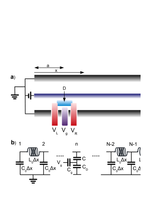
Figure 1: (Color online) a) Schematic of the system with a normal state metallic dot (D) inserted in a transmission line cavity a distance $a$ from the left end. The central conductor (blue) can be a superconductor or e.g. an array of SQUIDS. The dot is tunnel coupled to two metallic leads L,R (red) kept at voltages $V_{L}$ and $V_{R}$, respectively. The dot is capacitively coupled to a gate electrode (purple) kept at the voltage $V_{g}$. b) Discrete circuit representation of the dot-cavity system with $N$ nodes. The dot is connected to node $n$. The inductance between two adjacent nodes is $L_{0}\Delta x$ and the capacitance to ground from node $i\neq n$ is $C_{0}\Delta x$, giving the cavity a characteristic impedance $\sqrt{L_{0}/C_{0}}$. The dot-cavity capacitance is $C$, the dot-to-ground capacitances is $C_{D}$ and the gate capacitance is $C_{g}$.

II.1 Cavity-dot system

Our initial aim is to arrive at a Hamiltonian for the total system, without any approximation on the dot-cavity coupling strength. We start by considering the isolated dot-cavity system and derive a Hamiltonian expressed in terms of the charge on the dot, the photons in the cavity and the interaction between them. Following standard circuit QED procedure Yurke and Denker (1984); Devoret (1997) we first write down the Lagrangian for the circuit. We note that similar systems, with the focus on arbitrary strong dot-cavity coupling have been treated in e.g. Refs. Paladino et al., 2003; Koch et al., 2010. The discussion here is therefore kept short and details are presented only where our derivation differs from previous works.

The transmission line cavity is represented by a chain of $N\gg 1$ identical LC-circuits with capacitance $C_{0}\Delta x$ and inductance $L_{0}\Delta x$, where $\Delta x=d/N$. The quantum dot is coupled to the chain node $n=Na/d$ and to ground via capacitances $C$ and $C_{D}$, respectively. The Lagrangian of the circuit is then

$$L=\sum_{i\neq n}^{N}\frac{C_{0}\Delta x\dot{\phi}_{i}^{2}}{2}-\sum_{i}^{N-1}\frac{(\phi_{i+1}-\phi_{i})^{2}}{2L_{0}\Delta x}+\frac{C_{D}\dot{\phi}_{D}^{2}}{2}+$$

$$+\frac{C(\dot{\phi}_{n}-\dot{\phi}_{D})^{2}}{2}+\frac{C_{g}(V_{g}+\dot{\phi}_{D})^{2}}{2}$$ (1)

where $\phi_{i}$ is the phase of the i:th node and $\phi_{D}$ the phase of the dot.

To find the normal modesGoldstein et al. (2002) of the combined cavity-dot system we consider the Euler-Lagrange equations $\frac{d}{dt}\frac{\partial L}{\partial\dot{\phi}_{i}}-\frac{\partial L}{\partial\phi_{i}}=0$, for $i=1,..N,D$. Using the equation of $i=D$, $\ddot{\phi}_{D}$ can be expressed in terms of $\ddot{\phi}_{N}$ and substituted into the equation $i=N$. We can then write the equations for the cavity phases in matrix form

$$\mathcal{T}\mbox{\boldmath$\ddot{\phi}$}=\cal{V}\mbox{\boldmath$\phi$}$$ (2)

where $\mbox{\boldmath$\phi$}=[\phi_{1}..\phi_{N}]^{T}$ and the matrices $\cal{T},\cal{V}$ have elements $\mathcal{T}_{ij}=\delta_{ij}\left[C_{0}\Delta x+\frac{C(C_{0}\Delta x+C_{g})}{C+C_{D}+C_{g}}\delta_{in}\right]$ and $\mathcal{V}_{ij}=\frac{1}{L_{0}\Delta x}(\delta_{ij}(2-\delta_{i1}-\delta_{iN})-\delta_{i(j-1)}-\delta_{i(j+1)})$. Since $\mathcal{T}$ is diagonal with positive elements and $\cal{V}$ is real and symmetric we can express Eq. (2) in the basis of normal modes as $\mbox{\boldmath$\ddot{\varphi}$}=\Lambda\mbox{\boldmath$\varphi$}$, where $\mbox{\boldmath$\phi$}=M\mbox{\boldmath$\varphi$}$. The elements $\Lambda_{p}$ of the diagonal matrix $\Lambda$ are the frequencies of the normal modes squared, i.e. $\Lambda_{p}=\omega_{p}^{2}$. The columns, $\bf{m}_{p}$, in $M$ are the solutions to the eigenvalue problem

$$\mathcal{T}^{-1}\mathcal{V}{\bf{m}}_{p}=\omega_{p}^{2}{\bf{m}}_{p},$$ (3)

with the normalization condition ${\bf{m}}_{p}^{T}\mathcal{T}{\bf{m}}_{q}=C_{0}d\delta_{pq}$. We can then express the Lagrangian in terms of the normal modes as

$$L=\sum_{p}\left(\frac{C_{0}d\dot{\varphi}_{p}^{2}}{2}-\frac{C_{0}d\omega_{p}^{2}\varphi_{p}^{2}}{2}\right)+\frac{C^{2}}{2C_{\Sigma}}\sum_{pq}M_{np}M_{nq}\dot{\varphi}_{p}\dot{\varphi}_{q}$$

$$+C_{g}V_{g}\dot{\varphi}_{D}+\frac{C_{D}\dot{\varphi}_{D}^{2}}{2}-C\dot{\varphi}_{D}\sum_{p}M_{np}\dot{\varphi}_{p}$$ (4)

where $C_{\Sigma}=C_{D}+C+C_{g}$ and we write $\phi_{D}=\varphi_{D}$ for notational convenience.

In the continuum limit, $N\rightarrow\infty$, $\Delta x\rightarrow 0$ with $N\Delta x=d$ constant, the vectors $\bf{m}_{p}$ turn into continuous functions, $\zeta_{p}(x)$, of the coordinate $x$ along the transmission line. From Eq. (3) it is found that the functions $\zeta_{p}(x)$ satisfy the differential equation

$$\zeta_{p}^{\prime\prime}(x)+k_{p}^{2}[1+d\alpha\delta(x-a)]\zeta_{p}(x)=0,$$ (5)

with boundary conditions $\zeta_{p}^{{}^{\prime}}(0)=\zeta_{p}^{{}^{\prime}}(d)=0$. Here $k_{p}=\sqrt{L_{0}C_{0}}\omega_{p}$ and $\alpha=C_{g}C/(C_{\Sigma}C_{0}d)$. The normalization condition above becomes

$$\frac{1}{d}\int_{0}^{d}dx\zeta_{p}(x)\zeta_{q}(x)[1+\alpha d\delta(x-a)]=\delta_{pq}.$$ (6)

This generalized Sturm-Liouville problem has solutions

$$\zeta_{p}(x)=\left\{\begin{array}[]{cc}A_{p}\cos(k_{p}x)&0\leq x\leq a\\ B_{p}\cos[k_{p}(d-x)]&a\leq x\leq d,\end{array}\right.$$ (9)

where $A_{p}\cos(k_{p}a)=B_{p}\cos[k_{p}(d-a)]$ and $k_{p}$ are the positive solutions to the equation

$$\frac{\tan(k_{p}d)[1+\tan^{2}(k_{p}a)]}{1+\tan(k_{p}a)\tan(k_{p}d)}=-\alpha k_{p}d,$$ (10)

following from Eq. (5) with boundary conditions. The solutions are illustrated in Fig. 2. The normalization condition in Eq. (6) gives

$$A_{p}^{2}=\frac{d}{2}\left[a+\frac{\sin(2k_{p}a)}{2k_{p}}+\cos^{2}(k_{p}a)F_{p}\right]^{-1}$$ (11)

with

$$F_{p}=\frac{(d-a)}{\cos^{2}[k_{p}(d-a)]}+\frac{\tan[k_{p}\left(d-a\right)]}{2k_{p}}+\alpha d.$$ (12)

We see that in the limit $\alpha k_{p}d\ll 1$, corresponding to low frequencies $\omega_{p}$, the solutions $k_{p}$ in Eq. (10) approach $p\pi/d$, the result for the cavity disconnected from the dot. In the opposite limit, $\alpha k_{p}d\gg 1$, the solutions approach $(p+1/2)\pi/a$ and $(p+1/2)\pi/(d-a)$. This gives, from Eq. (9) that the amplitudes $\zeta_{p}(x)$, at $x=a$, will be zero: for large $\omega_{p}$ the cavity is effectively grounded via the dot.

Thus, in the continuum limit we obtain the Lagrangian for the system

$$L=\sum_{p}\left(\frac{C_{C}\dot{\varphi}_{p}^{2}}{2}-\frac{(k_{p}d)^{2}\varphi_{p}^{2}}{2L_{C}}\right)-C\dot{\varphi}_{D}\sum_{p}\zeta_{p}(a)\dot{\varphi}_{p}$$

$$+\frac{C^{2}}{2C_{\Sigma}}\sum_{pq}\zeta_{p}(a)\zeta_{q}(a)\dot{\varphi}_{p}\dot{\varphi}_{q}+\frac{C_{\Sigma}\dot{\varphi}_{D}^{2}}{2}+C_{g}V_{g}\dot{\varphi}_{D},$$

where $C_{C}=C_{0}d$ and $L_{C}=L_{0}d$ are the total capacitance and inductance of the cavity. This Lagrangian can now be used to obtain the conjugate variables $Q_{D}=\partial L/\partial\dot{\varphi}_{D}$ and $Q_{p}=\partial L/\partial\dot{\varphi}_{p}$ to $\varphi_{D}$ and $\varphi_{p}$ respectively. We point out that $Q_{D}$ is the charge on the dot.

Expressing $\dot{\varphi}_{D}$ and $\dot{\varphi}_{p}$ in terms of $Q_{D}$ and $Q_{p}$ and using the Legendre transformation, $H_{S}=Q_{D}\dot{\varphi}_{D}+\sum_{p}Q_{p}\dot{\varphi}_{p}-L$, the following classical Hamiltonian of the system is obtained:

$$H_{S}=\sum_{p}\left(\frac{Q_{p}^{2}}{2C_{C}}+\frac{(k_{p}d)^{2}\varphi_{p}^{2}}{2L_{C}}+\frac{C(Q_{D}-C_{g}V_{g})}{C_{\Sigma}C_{0}}\zeta_{p}(a)Q_{p}\right)$$

$$+\frac{(Q_{D}-C_{g}V_{g})^{2}}{2C_{\Sigma}}\left(1+\frac{C^{2}}{C_{\Sigma}C_{C}}\sum_{p}\zeta_{p}(a)^{2}\right).$$ (14)

The quantum Hamiltonian is obtained by canonical quantization. The generalized coordinates $Q_{p},\varphi_{p},Q_{D}$ and $\varphi_{D}$ are replaced by operators $\hat{Q}_{p},\hat{\varphi}_{p},\hat{Q}_{D}$ and $\hat{\varphi}_{D}$ and the commutation relations $[\hat{Q}_{p},\hat{\varphi}_{q}]=i\hbar\delta_{pq}$, for $p,q=D,1,2,..$, are imposed. For the coordinates of the cavity $\hat{\varphi}_{p},\hat{Q}_{p}$ creation and annihilation operators $\hat{a}_{p},\hat{a}_{p}^{{\dagger}}$ are introduced for $p=1,2,..$ according to

$$\hat{Q}_{p}=\sqrt{\hbar k_{p}d}\left(\frac{C_{0}}{L_{0}}\right)^{1/4}\frac{(\hat{a}_{p}^{{\dagger}}+\hat{a}_{p})}{\sqrt{2}}$$

$$\hat{\varphi}_{p}=i\sqrt{\frac{\hbar}{k_{p}d}}\left(\frac{L_{0}}{C_{0}}\right)^{1/4}\frac{(\hat{a}_{p}^{{\dagger}}-\hat{a}_{p})}{\sqrt{2}}.$$ (15)

These operators fulfill bosonic commutation relations $[\hat{a}_{p},\hat{a}^{{\dagger}}_{q}]=\delta_{pq}$. The Hamiltonian of the isolated dot-cavity system can then be written

$$\hat{H}_{S}=\underbrace{\sum_{p}\hbar\omega_{p}\hat{a}_{p}^{{\dagger}}\hat{a}_{p}}_{\hat{H}_{C}}+\underbrace{\frac{(\hat{Q}_{D}-C_{g}V_{g})^{2}}{2C_{\Sigma}}\left(1+\frac{C^{2}}{C_{\Sigma}C_{C}}\sum_{p}\zeta_{i}^{2}(a)\right)}_{\hat{H}_{D}}$$

$$+\underbrace{\frac{C(\hat{Q}_{D}-C_{g}V_{g})}{C_{\Sigma}}\sum_{p}\sqrt{\frac{\hbar\omega_{p}}{2C_{C}}}(\hat{a}_{p}+\hat{a}_{p}^{{\dagger}})\zeta_{p}(a)}_{\hat{H}_{DC}}.$$ (16)

This Hamiltonian has the desired form $\hat{H}_{S}=\hat{H}_{C}+\hat{H}_{D}+\hat{H}_{DC}$. The first term, $\hat{H}_{C}$, is the Hamiltonian of a set of harmonic oscillators corresponding to cavity modes with frequencies $\omega_{p}$. These frequencies are obtained by solving Eq. (10). The second term, $\hat{H}_{D}$, corresponds to the charging energy of the dot. We see that this is larger than for a dot with self-capacitance $C_{\Sigma}$. The third term in the Hamiltonian, $\hat{H}_{DC}$, is the linear coupling between the charge of the dot and the modes in the cavity. It is convenient for the further analysis to introduce the dimensionless coupling constant

$$\lambda_{p}=\frac{C}{C_{\Sigma}}\frac{e\zeta_{p}(a)}{\sqrt{2\hbar\omega_{p}C_{C}}}=\frac{C}{C_{\Sigma}}\sqrt{\frac{Z_{0}}{R_{q}}}\frac{\zeta_{p}(a)}{\sqrt{k_{p}d/(2\pi)}},$$ (17)

We emphasize that the Hamiltonian Eq. (16) has been obtained in an exact way, without any assumptions about the cavity-dot coupling strength. It is interesting to note, just as was done in Ref. Paladino et al., 2003, that this exact treatment gives a Caldeira-Leggett type Hamiltonian, naturally including the so called counter term. Weiss (2008) This counter term is typically introduced by hand to ensure a spatially uniform damping in the Caldeira-Leggett model. In our model the counter term just comes from the part of the charging energy term $\hat{H}_{D}$ arising from the normalization of the capacitance $C_{\Sigma}$.

II.2 Coupling to leads and Lang-Firsov transformation

As a next step we consider the tunnel coupling of the dot to external leads $L$ and $R$. Following the standard path for transport through single-electron-transistors, Ingold and Nazarov (1992) the orbital and charge degrees of freedom of the metallic dot are treated separately. We describe the orbital degrees of freedom by the Hamiltonian

$$H_{O}=\sum_{k^{\prime}}\epsilon_{Dk^{\prime}}\hat{c}^{{\dagger}}_{Dk^{\prime}}\hat{c}_{Dk^{\prime}},$$ (18)

where $\hat{c}_{Dk^{\prime}}^{{\dagger}}$ creates an electron with energy $\epsilon_{Dk^{\prime}}$ in the dot. The Hamiltonian of the leads is

$$\hat{H}_{L}=\sum_{\ell,k}\epsilon_{\ell k}\hat{c}^{{\dagger}}_{\ell k}\hat{c}_{\ell k},$$ (19)

where $\hat{c}^{{\dagger}}_{\ell k}$ is the creation operator of an (uncharged) electron with energy $\epsilon_{\ell k}$ in lead $\ell=L,R$. In Eqs. (18) and (19) the indices $k$ and $k^{\prime}$ denotes both wave number and spin. The tunnel Hamiltonian is written as

$$\hat{H}_{T}=\sum_{\ell,k,k^{\prime}}t_{\ell kk^{\prime}}\hat{c}_{\ell k}^{{\dagger}}\hat{c}_{Dk^{\prime}}\exp\left(\frac{ie\hat{\varphi}_{D}}{\hbar}\right)+h.c,$$ (20)

where the operators $\exp\left(\mp ie\hat{\varphi}_{D}/\hbar\right)$ has the effect of changing the dot charge by $\pm 1$. This yields a Hamiltonian of the total system

$$\hat{H}=\hat{H}_{O}+\hat{H}_{C}+\hat{H}_{D}+\hat{H}_{DC}+\hat{H}_{T}+\hat{H}_{L}.$$ (21)

For further analysis it is convenient to first perform a canonical transformation of $\hat{H}$ that removes the linear-in-charge term $\hat{H}_{DC}$. Such a Lang-Firsov, or polaron,Mahan (2000) transformation is carried out by transforming the Hamiltonian as $\bar{H}=\exp(\hat{s})\hat{H}\exp(-\hat{s})$ and state kets as $\ket{\bar{\Psi}}=\exp(-\hat{s})\ket{\Psi}$ with $\hat{s}=[(\hat{Q}_{D}-C_{g}V_{g})/e]\sum_{p}\lambda_{p}(\hat{a}_{p}^{{\dagger}}-\hat{a}_{p})$. We then arrive at the Hamiltonian

$$\bar{H}=\hat{H}_{L}+\hat{H}_{O}+\sum_{p}\hbar\omega_{p}\hat{a}_{p}^{{\dagger}}\hat{a}_{p}+\frac{(\hat{Q}_{D}-C_{g}V_{g})^{2}}{2C_{\Sigma}}$$

$$\!\!\!\!\!\!+\sum_{\ell,k,k^{\prime}}t_{\ell kk^{\prime}}\hat{c}_{\ell k}^{{\dagger}}\hat{c}_{Dk^{\prime}}\exp\left(\frac{ie\hat{\varphi}_{D}}{\hbar}\right)\exp\left[-\sum_{p}\lambda_{p}(\hat{a}_{p}^{{\dagger}}-\hat{a}_{p})\right]$$

$$+h.c,$$ (22)

The eigenstates of the isolated dot-cavity system, decoupled from the leads, are up to an unimportant phase factor given by

$$\ket{N\mathbb{n}}=\ket{N}_{el}\exp\left[N\sum_{p}\lambda_{p}(\hat{a}_{p}^{{\dagger}}-\hat{a}_{p})\right]\ket{\mathbb{n}},$$ (23)

the tensor product of the charge state with $N$ excess electrons on the dot, $\ket{N}_{el}$, and the Fock states of the cavity modes, $\ket{\mathbb{n}}=\ket{n_{1}n_{2}...}$, displaced by $N\lambda_{p}$ each. We refer to the states $\ket{N\mathbb{n}}$ as microwave polaron states and $n_{p}$ as the number of photons in mode $p$. The energies of the polarons are given by

$$\epsilon_{N\mathbb{n}}=\frac{e^{2}(N-n_{g})^{2}}{2C_{\Sigma}}+\sum_{p}n_{p}\hbar\omega_{p}$$ (24)

with $n_{g}=C_{g}V_{g}/e$. Looking at Eq. (24) we note that the shift in charging energy from the coupling to the cavity modes, a polaron shift, is exactly canceled by the extra charging energy due to the renormalization of the capacitance of the dot. This cancellation is a direct consequence of the exact treatment of the cavity-dot coupling throughout the derivation. If one instead of Eq. (16) naively would start with a standard Anderson-Holstein type Hamiltonian, i.e. without the renormalized capacitance $C_{\Sigma}$, and then perform the polaron transformation, the resulting charging energy term could become negative for large dot-cavity couplings. For a metallic dot, with a continuous density of states, such a model would be unphysical; the system would lack a well defined ground state since increasing the number of electrons on the dot always would lower the total energy of the system. It should be noted that problems with infinite negative energies typically do not appear in related electron-phonon models in molecular electronics.not

III Quantum master equation

From the Hamiltonian in Eq. (22) we can then derive a quantum master equation describing the dynamics of both the charge state in the dot and the state of the cavity modes. The derivation follows a standard path, see e.g. Refs. Gardiner and Zoller, 2004; Mitra et al., 2004; Rodrigues and Armour, 2005; Hübener and Brandes, 2009.

III.1 Derivation

In the rest of the paper we consider the case where the charging energy of the dot, $e^{2}/(2C_{\Sigma})$, is the largest energy in the system. It is then safe to assume that the number of excess electrons on the dot will only fluctuate between $N$ and $N+1$. For simplicity, we consider gate voltages such that $N$ can only take values 0 and 1. The difference in charging energy between states with $0$ and $1$ electrons is denoted $\Delta E_{C}$.

Starting from the Liouville equation for the density matrix, expanding to leading order in tunnel-coupling and tracing over reservoir and fermionic dot degrees of freedom we arrive at a quantum master equation for the elements of the reduced density matrix $\rho$ of the dot-cavity system. A more detailed derivation is presented in Appendix A. This equation is in the polaron basis given by

$$\frac{d}{dt}\braket{0\mathbb{n}}{\rho}{0\mathbb{m}}=-\frac{i}{\hbar}(\epsilon_{0\mathbb{n}}-\epsilon_{0\mathbb{m}})\braket{0\mathbb{n}}{\rho}{0\mathbb{m}}$$

$$+\sum_{\ell,\mathbb{k},\mathbb{l}} \Gamma_{\ell}[-h_{\ell}(\epsilon_{1\mathbb{l}}-\epsilon_{0\mathbb{k}})\prod_{p}X^{p}_{k_{p}l_{p}}X^{p}_{m_{p}l_{p}}\braket{0\mathbb{n}}{\rho}{0\mathbb{k}}$$

$$+g_{\ell}(\epsilon_{1\mathbb{l}}-\epsilon_{0\mathbb{m}})\prod_{p}X^{p}_{n_{p}k_{p}}X^{p}_{m_{p}l_{p}}\braket{1\mathbb{k}}{\rho}{1\mathbb{l}}$$

$$+g_{\ell}(\epsilon_{1\mathbb{k}}-\epsilon_{0\mathbb{n}})\prod_{p}X^{p}_{n_{p}k_{p}}X^{p}_{m_{p}l_{p}}\braket{1\mathbb{k}}{\rho}{1\mathbb{l}}$$

$$-h_{\ell}(\epsilon_{1\mathbb{k}}-\epsilon_{0\mathbb{l}})\prod_{p}X^{p}_{n_{p}k_{p}}X^{p}_{l_{p}k_{p}}\braket{0\mathbb{l}}{\rho}{0\mathbb{m}}]$$

$$\frac{d}{dt}\braket{1\mathbb{n}}{\rho}{1\mathbb{m}}=-\frac{i}{\hbar}(\epsilon_{1\mathbb{n}}-\epsilon_{1\mathbb{m}})\braket{1\mathbb{n}}{\rho}{1\mathbb{m}}$$

$$+\sum_{\ell,\mathbb{k},\mathbb{l}} \Gamma_{\ell}[-g_{\ell}(\epsilon_{1\mathbb{k}}-\epsilon_{0\mathbb{l}})\prod_{p}X^{p}_{l_{p}k_{p}}X^{p}_{l_{p}m_{p}}\braket{1\mathbb{n}}{\rho}{1\mathbb{k}}$$

$$+h_{\ell}(\epsilon_{1\mathbb{m}}-\epsilon_{0\mathbb{l}})\prod_{p}X^{p}_{k_{p}n_{p}}X^{p}_{l_{p}m_{p}}\braket{0\mathbb{k}}{\rho}{0\mathbb{l}}$$

$$+h_{\ell}(\epsilon_{1\mathbb{n}}-\epsilon_{0\mathbb{k}})\prod_{p}X^{p}_{k_{p}n_{p}}X^{p}_{l_{p}m_{p}}\braket{0\mathbb{k}}{\rho}{0\mathbb{l}}$$

$$-g_{\ell}(\epsilon_{1\mathbb{l}}-\epsilon_{0\mathbb{k}})\prod_{p}X^{p}_{k_{p}n_{p}}X^{p}_{k_{p}l_{p}}\braket{1\mathbb{l}}{\rho}{1\mathbb{m}}]$$

where $h_{\ell}(x)=(x-[\mu_{\ell}-\mu_{D}])/(\hbar\omega_{1})[\exp[(x-[\mu_{\ell}-\mu_{D}])/k_{B}T]-1]^{-1}$, $g_{\ell}(x)=\exp[(x-[\mu_{\ell}-\mu_{D}])/k_{B}T]h_{\ell}(x)$ and $\Gamma_{\ell}=2\pi|t_{\ell}|^{2}\nu_{\ell}\nu_{D}\omega_{1}$. Here, $\mu_{\ell}$ and $\mu_{D}$ are the chemical potentials of the leads and the dot, respectively. Moreover, we have assumed tunneling amplitudes independent of lead and dot energy, i.e. $t_{kk^{\prime}\ell}\approx t_{\ell}$ and $\nu_{\ell}$, $\nu_{D}$ denotes the density of states of lead $\ell$ and the dot, respectively. Furthermore

$$X^{p}_{nm}=\braket{n}{\exp[-\lambda_{p}(\hat{a}^{{\dagger}}_{p}-\hat{a}_{p})]}{m}=\frac{1}{\sqrt{m!}}e^{-\lambda_{p}^{2}/2}$$

$$\times\sum_{j=0}^{min(m,n)}\lambda^{n+m-2j}_{p}(-1)^{n-j}\left(\begin{array}[]{c}m\\ j\end{array}\right)\frac{\sqrt{n!}}{(n-j)!}$$ (28)

are the Franck-Condon factorsMahan (2000) for the p:th mode. These are the amplitudes for the transition from the state in mode $p$ going between polaron states with $n$ and $m$ quanta as the electron tunnels into or our of the dot. Formally $X^{p}_{nm}$ is given by the overlap of oscillator wavefunctions before and after the tunneling. We emphasize that Eq. (LABEL:gme) is a quantum master equation: it describes the dynamics of the polaron states as well as coherences between them.

III.2 Franck-Condon effect

From Eq. (28) we note that for all Franck-Condon factors $X^{p}_{nm}\propto\exp(-\lambda_{p}^{2}/2)$. This means that even if no photons are excited as the electrons tunnel into and out of the dot, $n=m=0$, the presence of the modes in the cavity will still affect transport via renormalized, suppressed tunneling rates. This Franck-Condon suppression of electron tunneling is a pure vacuum effect, a consequence of the tunneling charge having to displace all the oscillators in the cavity. We introduce the vacuum renormalized tunneling rates

$$\tilde{\Gamma}_{\ell}=\Theta\Gamma_{\ell},\quad\Theta=\exp(-\sum_{p}\lambda_{p}^{2}),$$ (29)

where $\Theta$ denotes the renormalization factor. It is convenient to also introduce the notation $Y^{p}_{nm}=\exp(\lambda_{p}^{2}/2)X^{p}_{nm}$ for the remaining part of the Franck-Condon factors for the $p$:th mode.

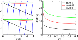
Figure 2: (Color online) Left panels: Intersections of the left and right hand side of Eq. (10), for different $\alpha$ (see right panel inset). The ratios $a/d=0$ and $a/d=1/4$ for upper and lower panel respectively. Right panel: Position dependence of the renormalization factor $-\ln(\Theta)/\gamma^{2}$, with $\gamma=(C/C_{\Sigma})\sqrt{Z_{0}/R_{q}}$. Only positions $0\leq a\leq d/2$ are plotted since the renormalization factor is symmetric with respect to $d/2$.

From Eq. (17) it follows that the coupling constant, $\lambda_{p}$, is proportional $\zeta_{p}(a)/\sqrt{k_{p}d}$. Consequently [see Eqs. (9) and (10)], the renormalization factor depends on the the distance $a$ and the parameter $\alpha=CC_{g}/(C_{\Sigma}C_{C})$. Since the dot can be placed at any position $a$, or effectively be moved by tuning the boundary conditions of the cavity,Wallquist et al. (2006); Sandberg et al. (2008) it is interesting to study the position dependence of $\Theta$, plotted in Fig. 2 for different values of $\alpha$. Several observations can be made: $(i)$ Albeit the renormalization factor can be large, it is always finite for $\alpha>0$. There is thus no tunneling orthogonality catastrophe, i.e zero over-lap between initial and final state in a tunneling event. Such an orthogonality catastrophe would occur if one naively replaces $\zeta_{p}(a)$ and $k_{p}$ with the corresponding amplitude, $\sqrt{2/d}\cos(p\pi a/d)$, and wavenumber $p\pi/d$, of the cavity disconnected from the dot. The exponent of the renormalization factor would then be proportional to $\sum_{p}\cos(p\pi/d)^{2}/p$ which diverges logarithmically. We emphasize that it is our exact treatment of the dot charge-cavity coupling fully taking into account the effect of the presence of the dot on the cavity modes that gives a finite $\tilde{\Gamma}_{\ell}$. $(ii)$ We see that the renormalization factor has a strong dependence on the distance $a$, with a minimum at $a=d/2$ and maximum at $a=0$. This is a consequence of that all modes have maximal amplitude, $\zeta_{p}(a)$, at $a=d$, while at $a=d/2$ half of the modes, i.e. the anti-symmetric, will have zero amplitude. $(iii)$ We note that $\Theta$ decreases with decreasing $\alpha$. This is to be expected, since a small $\alpha$ means that the amplitude of the cavity modes at the connection point remains finite for higher frequencies. It is also interesting to point out that a position dependence of the coupling constant was very recently investigated in the context of nano-electro mechanical systems. Traverso Ziani et al. (2011); Donarini et al. (2011)

III.3 Parameter regime

The quantum master equation in Eq. (LABEL:gme) allows us to investigate the charge and photon dynamics in a broad range of parameters. The main interest of the present work is to investigate new physical phenomena becoming important for strong dot-cavity coupling. This motivates us to focus on the deep quantum regime, with only a few photons in the cavity, where these phenomena can be investigated both qualitatively and quantitatively. Spelling out explicitly the parameter range, we consider symmetric tunnel couplings, $\Gamma_{L}=\Gamma_{R}=\Gamma$, and a symmetric bias $\mu_{L}=-\mu_{R}=eV/2$, giving a chemical potential of the dot $\mu_{D}=0$. We also consider the case where only the two lowest photon modes have finite populations. This restriction puts limits on the bias voltage; a careful investigation gives that $|eV/2\pm\Delta E_{C}|<\hbar\omega_{2}$ is necessary to guarantee a negligible occupation of the third and higher modes in all cases of interest. This condition means that it is energetically forbidden for a tunneling electron to emit a photon directly into the second mode. However, population of the second mode is still possible by inter-mode conversion of photons from the first mode, as discussed below. In the rest of the article we will use the simplified notation $\ket{Nn_{1}n_{2}}$ for the polaron states with $N=0,1$ electrons and $n_{1},n_{2}$ photons in the first and second mode, respectively.

We further assume that the tunneling rate is much smaller than the fundamental cavity frequency, i.e $\tilde{\Gamma}\ll\omega_{1}$. For the case where only the first photon mode is active, the off-diagonal elements $\braket{\mu n_{1}0}{\rho}{\mu m_{1}0}$, with $n_{1}\neq m_{1}$, of the steady state density matrix in Eq. (LABEL:gme) are a factor $\sim\tilde{\Gamma}/\omega_{1}\ll 1$ smaller than the diagonal elements and can be disregarded. This amounts to performing a secular, or rotating-wave, approximation and reduces Eq. (LABEL:gme) to a standard master equation. For two active modes the situation is different since two polaron states $\ket{Nn_{1}n_{2}}$ and $\ket{Nm_{1}m_{2}}$ can be degenerate, i.e. for $n_{1}\omega_{1}+n_{2}\omega_{2}-(m_{1}\omega_{1}+m_{2}\omega_{2})\ll\tilde{\Gamma}$ the secular approximation can not be performed. The off-diagonal density matrix elements $\braket{Nn_{1}n_{2}}{\rho}{Nm_{1}m_{2}}$, corresponding to coherences between polaron states with different number of photons, must thus be retained in Eq. (LABEL:gme). The simplest case giving degeneracy, discussed in detail below, occurs for $\alpha\ll 1$ when from Eq. (10) $\omega_{2}\approx 2\omega_{1}$. Moreover, to highlight the effect of the coherences we compare in several cases below the results based on Eq. (LABEL:gme) to the results based on a master equation where the off-diagonal elements are disregarded from the outset.

A key parameter in our work is the coupling constant, $\lambda_{1}$. To reach the strong coupling regime, the time scale for tunnel induced excitation and relaxation of the cavity photons must be much shorter than the intrinsic relaxation time. This amounts to the restriction

$$\sqrt{\kappa/\tilde{\Gamma}}\ll\lambda_{1},$$ (30)

on the coupling constant, where $\kappa=\omega_{1}/(2\pi Q)$ is the intrinsic relaxation rate of the first cavity mode and $Q$ the quality factor. To provide a concrete estimate, for reasonable parameters of a superconducting transmission line cavity $\omega_{1}/2\pi=10$GHz, $Q=10^{6}$, $Z_{0}=100\Omega$ and $C\sim C_{\Sigma}$ one has $\kappa=10$kHz and $\lambda_{1}=0.06$. Then, for a tunneling rate $\tilde{\Gamma}=200$MHz, the left-hand side of Eq. (30) is an order of magnitude smaller than the right-hand side.

The ultrastrong regime requires the coupling constant $\lambda_{1}$ to be of order unity. For the capacitive dot-cavity coupling considered here it has however been pointed out Devoret et al. (2007); Schoelkopf and Girvin (2008) that standard superconducting transmission lines only allow couplings $\lambda_{1}$ up to a few percent. The limiting factor, clear from Eq. (17), is the ratio $Z_{0}/R_{q}\ll 1$. To reach larger couplings one thus has to consider ways of increasing the characteristic impedance $Z_{0}$ of the transmission line. One promising possibility is transmission lines with a central conductor consisting of an array of Josephson junctions or SQUIDS acting as linear inductors. In recent experiments with SQUID array conductors Castellanos-Beltran and Lehnert (2007); Castellanos-Beltran et al. (2008) $Z_{0}\approx 6k\Omega$, i.e. $Z_{0}/R_{q}\approx 0.25$ was demonstrated, which would correspond to $\lambda_{1}$ of the order of tens of percent for a dot capacitively coupled to the transmission line. It should however be pointed out that in such high impedance transmission lines non-linear effects, not accounted for in our model, start to become relevant.

The relation between the coupling constants $\lambda_{1}$ and $\lambda_{2}$ is determined by Eq. (17) and Eq. (10) as

$$\frac{\lambda_{2}}{\lambda_{1}}\approx\frac{\cos(2\pi a/d)}{\cos(\pi a/d)},$$ (31)

for $\alpha\ll 1$. This relation is thus specified by $a$. Below we will consider two important qualitatively distinct cases, $a=d/4$ and and $a=0$. For $a=d/4$ we have $\lambda_{2}=0$ and only a the first mode has finite population. The case $a=0$ corresponds to a position in the cavity yielding maximal coupling strength. Eq. (31) then gives $\lambda_{1}=\sqrt{2}\lambda_{2}$ and both the first and the second mode can have finite population.

IV State of the photon modes of the cavity

We first consider the current-induced photon state in the cavity, the electronic transport is considered below. Experimentally, the photon state in the cavity can e.g. be investigated by capacitively coupling the cavity to a transmission line and measuring the state of the output itinerant modes.Bozyigit et al. (2010) This gives access to the frequency resolved population,Hofheinz et al. (2011) as well as higher moments of the cavity field via e.g. quantum state tomography of oneEichler et al. (2011a) or twoEichler et al. (2011b) itinerant modes. Moreover, the photon number Hofheinz et al. (2008) as well as the full photon state, Hofheinz et al. (2009) can also be obtained by coupling the cavity to a superconducting qubit, embedded in the cavity. Studying specific experimental setups to extract information about the photon state is however out of the scope of the present article. Hence we concentrate on the photon state of the cavity described by the steady-state density matrix, obtained from Eq. (LABEL:gme).

IV.1 Single-mode

We first consider the case of a single active mode, obtained when the coupling strength for the second mode is zero, i.e $\lambda_{2}=0$. To demonstrate the effect of the tunneling electrons on the state of the first mode it is instructive to consider the average number of photon excitations in the two polaron states, $n_{ph}=\sum_{n}nP_{n}$ with $P_{n}=\braket{0n0}{\rho_{s}}{0n0}+\braket{1n0}{\rho_{s}}{1n0}$ and $\rho_{s}$ the steady-state density matrix. The average number of excitations, $n_{ph}$, is related to the photon population in the unrotated basis $\braket{\hat{n}_{1}}$ as $\braket{\hat{n}_{1}}=n_{ph}+\lambda_{1}^{2}\sum_{n}\braket{1n0}{\rho_{s}}{1n0}$. In Fig. 3 $n_{ph}$ is plotted against the bias voltage for different coupling strengths, $\lambda_{1}$. Considering the curves corresponding to charge degeneracy i.e. $\Delta E_{C}=0$, we note that $n_{ph}$ is zero until the bias voltage, $eV$ reaches $2\hbar\omega_{1}$, after which it starts to increase continuously with bias voltage. For the curves corresponding to $\Delta E_{C}=0.25\hbar\omega_{1}$ the onset occurs at $eV=1.5\hbar\omega_{1}$ and there is an additional kink on each curve at $eV=2.5\hbar\omega_{1}$.

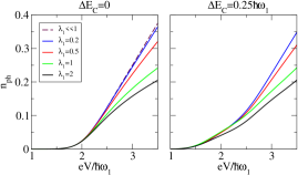
Figure 3: (Color online) Mean number of photon excitations $n_{ph}$ for a single active mode $(\lambda_{2}=0)$ as a function of bias voltage $eV$ for different coupling strengths $\lambda_{1}$ and charging energy differences $\Delta E_{C}=0$ (left) and $0.25\hbar\omega_{1}$ (right). The temperature is $k_{B}T=0.05\hbar\omega_{1}$. In the left panel the dashed line gives the analytical result Eq. (34) for $eV-2\hbar\omega_{1}\gg k_{B}T$.

These onsets and kinks can be understood from the energetics of allowed tunneling processes: Due to the continuous density of states of the dot all electrons in the lead with energies above $\Delta E_{C}$, can tunnel into the dot. Photon emission by the tunneling electrons is however only possible for electrons with energies above $\hbar\omega_{1}+\Delta E_{C}$. Similarly, an electron in the dot can tunnel out to unoccupied states in the leads with energies below $\Delta E_{C}$, but can only tunnel out with photon emission to states with energies below $\Delta E_{C}-\hbar\omega_{1}$. Therefore, at low temperatures photon emission is only possible by an electron tunneling from (to) the left (right) lead for a bias voltages $eV/2\geq\hbar\omega_{1}+(-)\Delta E_{C}/2$. The onsets and kinks in Fig. 3 thus correspond to thresholds of tunneling processes with photon emission into the cavity.

The rate of increase of the population $n_{ph}$ with increasing $eV>2\hbar\omega_{1}-\Delta E_{C}$ can most easily be understood for $\Delta E_{c}=0$. We see in Fig. 3 that the population goes from growing almost linearly for $\lambda_{1}=0.2$ to a slower, sub linear increase for larger $\lambda_{1}\sim 1$. In the limit $\lambda_{1}\ll 1$ an analytical formula for the photon distribution, $\{P_{n}\}$, can be derived by only taking into account processes to leading order in $\lambda_{1}$ (see Appendix C). For $eV-2\hbar\omega_{1}\gg k_{B}T$ we obtain

$$P_{n}=\frac{2\hbar\omega_{1}}{eV+2\hbar\omega_{1}}\left(\frac{eV-2\hbar\omega_{1}}{eV+2\hbar\omega_{1}}\right)^{n},$$ (32)

independent of $\lambda_{1}$. We note that the probabilities, $P_{n}$, are Boltzmann distributed. Hence the distribution can be described by an effective temperature

$$k_{B}T_{\text{eff}}=\hbar\omega_{1}/\ln[(eV+2\hbar\omega_{1})/(eV-2\hbar\omega_{1})].$$ (33)

Using standard thermodynamics we then obtain the following linear relation between the population and bias voltage as

$$n_{ph}=\frac{1}{\exp\left(\hbar\omega_{1}/[k_{B}T_{\text{eff}}]\right)-1}=\frac{eV-2\hbar\omega_{1}}{4\hbar\omega_{1}}.$$ (34)

Looking at Fig. 3 we see that $n_{ph}$ is well described by Eq. (34) for coupling strengths up to $\lambda_{1}\approx 0.2$. The slower increase with voltage for larger $\lambda_{1}$ can be understood as follows: In the limit $\lambda_{1}\ll 1$ only processes where the number of photons are changed $-1,0$ or $1$ are important, since they are the only ones having non-zero amplitude to leading order in $\lambda_{1}$. This is deduced from the corresponding Franck-Condon factors [see Eq. (28)]. However, at the considered bias voltages only processes where the number of photons is increased by at most one are allowed energetically. Thus, when $\lambda_{1}$ is increased the rate for the higher order processes where the photons number is decreased becomes larger, but not for the ones where the photon number is increased. Hence, the population $n_{ph}$ is decreased. The results are qualitatively similar for $\Delta E_{C}=0.25\hbar\omega_{1}$.

To further investigate the properties of the distribution, $\{P_{n}\}$ for coupling strengths approaching $\lambda_{1}\sim 1$, $P_{n}$ is plotted against $n$ for bias $eV=3\hbar\omega_{1}$ in Fig. 4. We see that the distribution decreases exponentially with $n$ for couplings $\lambda_{1}\ll 1$ in line with Eq. (32). For stronger couplings the decrease is faster, due to higher order relaxation processes. This observation shows that the probabilities $P_{n}$ are not Boltzmann distributed and hence an effective temperature cannot be defined. The cavity mode is thus clearly in a non-thermal state. This can be further illustrated by investigating e.g. the photon Fano factorMerlo et al. (2008) (not presented here).

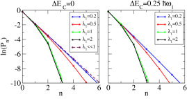
Figure 4: (Color online) Logarithm of the probability of $n$ photons for different coupling strengths and $\Delta E_{C}=0$ (left) $\Delta E_{C}=0.25\hbar\omega_{1}$ (right) for bias voltage $eV=3\hbar\omega_{1}$ and $k_{B}T=0.05\hbar\omega_{1}$.

An important feature of the photon state, not captured in the above analysis, is that an electron tunneling into the dot displaces the harmonic oscillator corresponding to the first cavity mode by an amount proportional to the coupling strength, $\lambda_{1}$. To illustrate the effect of the displacement of the mode we plot in Fig. 5 the Wigner-functionCahill and Glauber (1969)

$$W(\beta)=\int{\frac{d^{2}\xi}{\pi}}\operatorname{tr}\left(\rho_{s}\exp\left[\xi\hat{a}_{1}^{\dagger}-\xi^{*}\hat{a}_{1}\right]\right)\exp\left(\xi\beta^{*}-\xi^{*}\beta\right),$$ (35)

where the trace is taken over both electron and photon degrees of freedom. From Fig. 5 we note that for coupling $\lambda_{1}=0.2$, we can only discern a single peak of the Wigner function while for the larger coupling, $\lambda_{1}=2$, the peak is split into two. The second peak comes from the photons of the polaron of the charged dot and it becomes visible for coupling strengths $\lambda_{1}\sim 1$. We also note that $\Delta E_{C}$ has an impact on the photon distribution as the second peak is weaker for $\Delta E_{C}=0.25\hbar\omega_{1}$ than for $\Delta E_{C}=0$. This is a consequence of a smaller probability of the dot being occupied in the previous case.

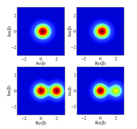
Figure 5: (Color online) Wigner function $W(\beta)$ for coupling strengths $\lambda_{1}=0.2$ (upper panel) and $2$ (lower panel) and charging energy differences $\Delta E_{C}=0$ (left) and $0.25\hbar\omega_{1}$ (right). The color scale goes from blue (small value) to red (large value). The bias voltage is $eV=3\hbar\omega_{1}$ and the temperature is $k_{B}T=0.05\hbar\omega_{1}$.

It is interesting to briefly compare our results to those obtained for the current-induced non-equilibrium state of a single boson mode coupled to a single-level, see e.g. Refs. Mitra et al., 2004; Hartle and Thoss, 2011a; Koch et al., 2006; Hartle and Thoss, 2011b. For a single-level dot, in contrast to our metallic dot, the population grows stepwise with bias voltage, where each step corresponds to an onset of photon emission in a tunneling process. Furthermore, in contrast our result Eq. (34), the photon distribution and hence the population is not convergent for charge degeneracy, $\Delta E_{C}=0$, in the limit of couplings, $\lambda_{1}\ll 1$, for voltages above the first onset of photon emission. Koch et al. (2006); Hartle and Thoss (2011a) This is because the rate for going from a state with $n$ to a state with $n+1$ photons is equal to the rate for the opposite process, which gives an equal probability of all photon states. In metallic dot the processes $n+1\rightarrow n$ has larger rate than $n\rightarrow n+1$, as discussed in detail in Appendix C.

IV.2 Two active modes

We then turn to the case with two active modes with $\lambda_{1}=\sqrt{2}\lambda_{2}$. As for the single-mode case, we first consider the average number of photon excitations in the two polaron states, defined by $n_{ph1(2)}=\sum_{n,m}n(m)\left[\braket{0nm}{\rho_{s}}{0nm}+\braket{1nm}{\rho_{s}}{1nm}\right]$. The dependence of $n_{ph1}$ and $n_{ph2}$ on bias voltage for different coupling strengths are depicted in Fig. 6. We see that the onsets and slopes in the curves for $n_{ph1}$ show the same qualitative behavior as in the single mode case. Moreover, importantly $n_{ph2}$ have onsets and kinks at the same bias voltages. This is despite the fact that direct excitation of this mode is not energetically allowed at the considered bias voltages. The population in the second mode is thus due to inter-mode conversion. The mechanism of this conversion is that a tunneling electron excites a photon in the second mode and simultaneously de-excites a photon in the first mode. Since the change of the energy of the tunneling electron is the same as when it emits a photon into the first mode, both process become energetically allowed at the same bias voltage. We note from Fig. 6 that $n_{ph2}$ initially increases with $\lambda_{1}=1$ up to and starts to decrease again, for even large $\lambda_{1}=2$. We also point out that there is a difference between the results obtained from calculations with and without the coherences retained. This is particularly apparent for the coupling strength $\lambda_{1}=1$. Here $n_{ph1}$ and $n_{ph2}$ are larger and significantly larger, respectively, in the presence of coherences. To identify the dependence of the coherent effects on the coupling strengths we plot the difference between the coherent and the incoherent occupations $n_{ph1}$ and $n_{ph2}$ as a function of $\lambda_{1}$ and $\lambda_{2}$ for bias voltage $eV=3\hbar\omega_{1}$ in Fig. 7.

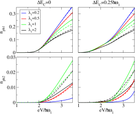
Figure 6: Color online). Mean number of photons in first and second mode, $n_{ph1},n_{ph2}$, against bias voltage for different coupling strengths and $\Delta E_{C}$. The temperature is $k_{B}T=0.05\hbar\omega_{1}$. Solid (dashed) lines show results with (without) coherences retained.

Polaron coherences

As is clear from both Figs. 6, 7, the effect of coherences on $n_{ph1}$ and $n_{ph2}$ are most pronounced around $\lambda_{1}=1$, for which they are enhanced. For the coupling strength to the second mode, the effect of the coherence is maximal around $\lambda_{2}\sim 1$ for $n_{ph1}$, while the effect on $n_{ph2}$ is maximal for $\lambda_{2}\ll 1$. A representative pair of couplings giving large coherence effects is $\lambda_{1}=1$ and $\lambda_{2}=1/\sqrt{2}$. For these specific coupling strengths a detailed investigation of the coherences can be performed. By a careful inspection of the numerically obtained steady-state density matrix for voltages above onset we find that only a limited number of polaron states have non-negligible amplitude. This allows us to describe the long-time charge and photon properties by an effective master-equation

$$\frac{d\mathbb{P}}{dt}=M\mathbb{P},$$ (36)

where $\mathbb{P}=[P_{000},\quad P_{010},\quad P_{0\Omega},\quad P_{100},\quad P_{110},\quad P_{1\Phi}]^{T}$, with $P_{\mu 00},P_{\mu 10}$, $P_{0\Omega}$ and $P_{1\Phi}$ being the probabilities for the states $\ket{\mu 00},\ket{\mu 10}$, $\ket{0\Omega}$ and $\ket{1\Phi}$, respectively. The latter states are given by

$$\ket{0\Omega}=\frac{\ket{020}-\ket{001}}{\sqrt{2}},\quad\ket{1\Phi}=\frac{\ket{120}+\ket{101}}{\sqrt{2}},$$ (37)

and are thus superpositions of degenerate polaron states with two photons in the first mode and one photon in the second mode. The matrix $M$ in Eq. (36) is further given by

$$M/\tilde{\Gamma}=$$

$$\!\!\!\!\!\!\!\!\!\!\!\!\!\begin{pmatrix}-\underset{j=0,1}{\sum}\tilde{h}_{j}&0\!\!\!&0\!\!&\tilde{g}_{0}&\tilde{g}_{1}&\!\!\!\!\!\!\!\!\!\!\!0\\ 0&-\underset{j=-1,1}{\sum}\!\!\!\!\tilde{h}_{j}\!\!\!&0&\tilde{g}_{-1}&0&\!\!\!\!\!\!\!\!\!\!\!\tilde{g}_{1}\\ 0&0\!\!&-\underset{j=-1,0}{\sum}\!\!\!\!\tilde{h}_{j}\!\!\!&0\!\!&\tilde{g}_{-1}&\!\!\!\!\!\!\!\!\!\!\!\!\tilde{g}_{0}\\ \!\!\!\tilde{h}_{0}&\tilde{h}_{-1}\!\!&0\!\!&-\underset{j=0,-1}{\sum}\!\!\!\!\tilde{g}_{j}&0&\!\!\!\!\!\!\!\!\!\!0\\ \tilde{h}_{1}&0&\tilde{h}_{-1}\!\!&0\!\!&-\underset{j=-1,1}{\sum}\!\!\!\!\tilde{g}_{j}&\!\!\!\!\!\!\!\!\!\!0\\ 0&\tilde{h}_{1}&\tilde{h}_{0}\!\!&0\!\!&0\!\!&\!\!\!\!\!\!\!\!-\underset{j=0,1}{\sum}\tilde{g}_{j}\end{pmatrix},$$ (38)

where $\tilde{h}_{j}=\sum_{\ell=L,R}h_{\ell}(j\hbar\omega_{1}+\Delta E_{C})$ and $\tilde{g}_{j}=\sum_{\ell=L,R}g_{\ell}(j\hbar\omega_{1}+\Delta E_{C})$.

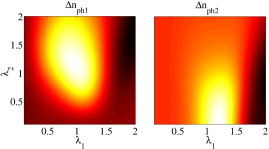
Figure 7: (Color online) The difference between the obtained average number of excitations in the first mode $n_{ph1}$ (left) and second mode $n_{ph2}$ (right) when coherences are retained and not in the quantum master equation. The color scale goes from black (small difference) to white (large difference). The bias voltage is $eV=3\hbar\omega_{1}$ and temperature $k_{B}T=0.05\hbar\omega_{1}$.

To illustrate the origin of the coherences in the master equation, the transitions described by Eq. (36) are depicted in Fig. 8. For comparison, the transitions of the corresponding incoherent master equation, with probabilities $P_{\mu 00}$, $P_{\mu 10}$, $P_{\mu 20}$ and $P_{\mu 01}$, are shown to the right. The transitions between states with an energy in the cavity modes less or equal to $\hbar\omega_{1}$ are the same in the coherent and incoherent case. For transitions to, from or between states with an energy $2\hbar\omega_{1}$ in the cavity modes, however, the picture is different. Consider e.g. the transition from $\ket{110}$ in which an additional quanta, $\hbar\omega_{1}$, is excited in the cavity modes. Two processes contribute to this transition: An additional photon can be excited in the first mode, $\ket{110}\rightarrow\ket{020}$, and a photon can be excited in the second mode by inter-mode conversion $\ket{110}\rightarrow\ket{001}$. Since $\ket{020}$ and $\ket{001}$ are degenerate the final state is a superposition of them in the coherent case, $\ket{0\Omega}$, while there is no superposition in the incoherent case. Similar explanations hold for the other transitions to, from or between states with energy $2\hbar\omega_{1}$.

From Eq. (36) an expression for the steady-state density matrix, $\rho_{s}$, can be obtained. Considering e.g. $\Delta E_{C}=0$ and $eV-2\hbar\omega_{1}\gg k_{B}T$ the steady- state density matrix has the simple form

$$\rho_{s}=\frac{1}{2}\frac{1}{3(eV)^{2}+4(\hbar\omega_{1})^{2}}$$

$$\times[\left(\ket{000}\bra{000}+\ket{100}\bra{100}\right)(eV+2\hbar\omega_{1})^{2}$$

$$+\left(\ket{010}\bra{010}+\ket{110}\bra{110}\right)\left[(eV)^{2}-4(\hbar\omega_{1})^{2}\right]$$

$$+[\ket{0\Omega}\bra{0\Omega}+\ket{1\Phi}\bra{1\Phi}][eV-2\hbar\omega_{1}]^{2}].$$ (39)

This expression clearly shows that the superpositions of polaron states have finite probabilities. We point out that $\ket{0\Omega}$ is an odd superposition while $\ket{1\Phi}$ is even [see Eq. (37)]. The amplitudes for the two states in the superposition are determined by the Franck-Condon factors for the two processes [see Eq.(LABEL:gme)]. The steady-state density matrix thus displays non-trivial correlations between the cavity photon state and the charge state of the dot. From Eq. (39) we also find the populations

$$n_{ph1}=\frac{2eV(eV-2\hbar\omega_{1})}{3(eV)^{2}+4(\hbar\omega_{1})^{2}}$$

$$n_{ph2}=\frac{1}{2}\frac{(eV-2\hbar\omega_{1})^{2}}{3(eV)^{2}+4(\hbar\omega_{1})^{2}},$$ (40)

in good agreement with the numerical results in Fig. 6.

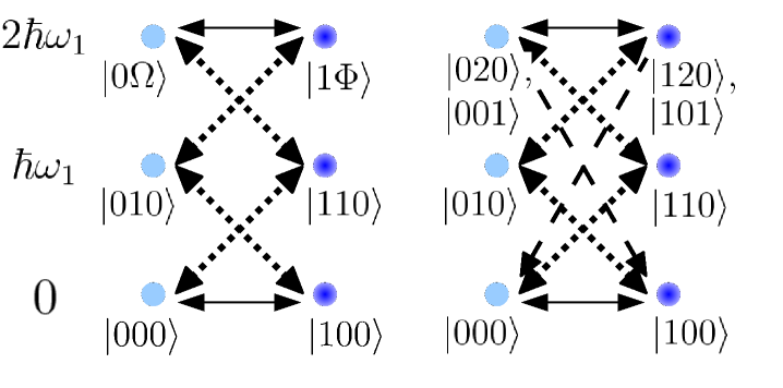
Figure 8: (Color online) Scheme of transition between different states for the effective master equation Eq. (36) (left) and the corresponding incoherent master equation (right). The filled lines represents transitions when no photon is emitted or absorbed, the dotted lines represent transitions involving one photon. The dashed lines represents transitions where two photons are emitted.

To understand qualitatively the effect of the coherences on the populations we again consider Fig. 8. We see that the major difference between the coherent and incoherent master equation is that there is no direct relaxation from states with energy $2\hbar\omega_{1}$ to states with zero energy in the photon modes in the former case. This coherent blocking of relaxation provides a plausible explanation of why $n_{ph1}$ and $n_{ph2}$ are enhanced for this case (see Fig. 6).

V Electronic transport and noise

Having investigated the current-induced non-equilibrium photon state we now turn to the properties of the electronic transport itself, fully accounting for the back-action of the cavity photons on the tunneling electrons. We focus our investigation on the average current and the low frequency current fluctuations, or noise, Blanter and Büttiker (2000) experimentally accessible in metallic quantum dots.Kafanov and Delsing (2009) The current $I$ and the noise $S$ can conveniently be calculated from the number resolved version of the quantum master equation Eq. (LABEL:gme), as discussed in the context of full counting statistics, see e.g. early works Bagrets and Nazarov (2003); Flindt et al. (2005); Kießlich et al. (2006); Braggio et al. (2006) for a detailed discussion. For completeness of the present work we give in Appendix B a short derivation of the expressions for the current and the noise, used in the analytical and numerical calculations below.

Conductance and noise for a single active mode

We first consider the I-V characteristics when only a single mode is active, i.e. $\lambda_{2}=0$. In Fig. 9 the conductance $G=dI/dV$ is plotted against bias voltage for different coupling strengths and charging energy differences $\Delta E_{C}$. The main feature of the conductance is a stepwise increase as the bias voltage passes $2\hbar\omega_{1}$ and $(2\pm 0.5)\hbar\omega_{1}$ for $\Delta E_{C}=0$ and $\Delta E_{C}=0.25\hbar\omega_{1}$, respectively. As concluded in the last section, at these bias voltages photon emission in the tunneling process becomes energetically allowed. In the low bias regime, $eV<2\hbar\omega_{1}-\Delta E_{C}$, the cavity modes effect the transport only by renormalizing the tunneling rate [Franck-Condon effect see Eq. (29)]. Considering specifically $\Delta E_{C}=0$ the conductance is

$$G_{0}=\frac{e^{2}\tilde{\Gamma}}{4\hbar\omega_{1}}$$ (41)

for any $\lambda_{1}$. For $eV>2\hbar\omega_{1}$ the electrons can also tunnel by emitting or absorbing a photon in the first mode. Thus, additional transport channels open up which gives the increase in conductance. For $\lambda_{1}\ll 1$ an analytical formula can be derived for the conductance (see Appendix C). For bias voltages $eV-2\hbar\omega_{1}\gg k_{B}T$, the conductance is given by

$$G_{1}=\frac{e^{2}\tilde{\Gamma}(1+\lambda_{1}^{2})}{4\hbar\omega_{1}}.$$ (42)

Thus, the contribution from the additional channels scales as $\lambda_{1}^{2}$. This dependence derives from the rate of emission or absorption of one photon in a tunneling event, proportional to $|Y_{nn+1}^{1}|^{2}\propto\lambda_{1}^{2}$. Interestingly, the result in Eq. (42) is independent on the distribution $\{P_{n}\}$. For larger coupling strengths $\lambda_{1}\sim 1$ processes of higher order in $\lambda_{1}$ start to contribute to the conductance and Eq. (42) no longer holds. The rate of tunneling into and out of the dot will be dependent on the number of photons in the cavity, i.e. the conductance becomes dependent on the distribution $\{P_{n}\}$. As is seen in Fig. 9, the higher order processes typically lead to an increased conductance.

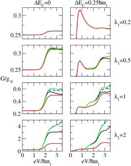
Figure 9: (Color online) Differential conductance as a function of bias voltage, in units of $g_{0}=e^{2}\tilde{\Gamma}/\hbar\omega_{1}$. The results are obtained by a quantum master equation for one mode (black), two modes without coherences (dashed blue), two modes with coherences (green) and for an equilibrated photon distribution at temperature $k_{B}T_{ph}\ll\hbar\omega_{1}$ (red). The electron temperature was $k_{B}T=0.05\hbar\omega_{1}$.

To gain further insight into the effect of the coupling to the photon mode on the electron transport properties, we investigate the correlations between the tunneling electrons. The correlations are quantified by the Fano-factor $F=S/(eI)$. For a dot decoupled from the cavity the electrons are anti-correlated due to the Coulomb interaction, and F is always less than one for bias voltage $eV-\Delta E_{C}\gg k_{B}T$. The Fano-factor for the dot coupled to a single photon mode is plotted against bias voltage in Fig. 10. Below the onset voltage the only effect of the coupling between the dot and the cavity mode is a renormalization of the tunneling rates. Focusing on $\Delta E_{C}=0$, the noise is

$$S=\frac{e^{3}V\tilde{\Gamma}}{8\hbar\omega_{1}},$$ (43)

giving a Fano-factor $1/2$. Above onset, i.e. for bias voltages $eV-2\hbar\omega_{1}\gg k_{B}T$, the noise becomes dependent on the coupling strength $\lambda_{1}$. In the limit $\lambda_{1}\ll 1$ an expression for the noise can be found analytically (See Appendix C). We find

$$S=\frac{e^{2}\tilde{\Gamma}}{4\hbar\omega_{1}}\left(\frac{eV(1+\lambda_{1}^{2})}{2\hbar\omega_{1}}-\lambda_{1}^{2}\right)=\frac{eI}{2}$$ (44)

which gives a Fano-factor of $1/2$ above the onset voltage as well. Thus, the onset of photon emission does not change the correlations between the tunneling electrons. We point out that corrections to the Fano-factor in Eq. (44) is of order $\lambda_{1}^{4}$. Consequently, as can be seen in Fig. 10, the deviation in the Fano-factor from $1/2$ for $\Delta E_{C}=0$ is small even for coupling strengths as large as $\lambda_{1}=0.5$. However, for coupling strengths approaching $\lambda_{1}\sim 1$ we see an increase in the Fano-factor as the bias voltage passes $2\hbar\omega_{1}$ and for $\lambda_{1}=2$ we even get super-poissonian noise. Similarly we see for $\Delta E_{C}=0.25\hbar\omega_{1}$ that there is an increase in the Fano-factor for the bias voltage $1.5\hbar\omega_{1}$ for coupling strengths $\lambda_{1}\sim 1$.

Thus, the change in the Fano-factor above the onset voltage occurs for coupling strengths deep into the ultrastrong coupling regime, $\lambda_{1}\sim 1$. To understand this we recall that the tunneling into and out of the dot is dependent on the photon state for these coupling strengths. For e.g. two subsequently tunneling electrons this means that the tunneling rate for the later electron depends on which photon state the cavity mode was left in by the first electron. For the parameter regime investigated, this leads to an increased tendency of bunching, and hence a larger Fano-factor. In an equivalent physical picture the increase in the Fano-factor can be attributed to the emergence of the avalanche effect found for a single level strongly coupled to a boson mode described in Ref. Koch and von Oppen, 2005a. We thus find that the effect is also present for a metallic dot coupled to a boson mode.

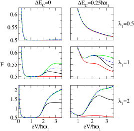
Figure 10: (Color online) Fano-factor as a function of bias voltage obtained for one mode (black), two modes without coherences (dashed blue), two modes with coherences (green) and for the first mode being equilibrated (red). The temperature was $k_{B}T=0.05\hbar\omega_{1}$.

To highlight the effect of the non-equilibrium photon distribution on the transport properties it is instructive to compare the result presented above to ones where the cavity modes are equilibrated at $T_{ph}$. (see Appendix D for details). To keep the discussion short we focus the discussion on temperatures $T_{ph}$ for which only the first mode can have a finite thermal population and $\Delta E_{C}=0$. We consider first the conductance $G^{th}$ and restate that for coupling strengths $\lambda_{1}\ll 1$ the conductance is independent on the photon distribution. Hence the conductance for an equilibrated mode is given by Eqs. (41) and (42) below and above the onset voltage, respectively. For larger coupling strengths, $\lambda_{1}\sim 1$, when the photon distribution affects the transport, the conductances for equilibrated and non-equilibrated modes differ. For bias voltages below the onset voltage the conductance is given by

$$G^{th}_{0}=\frac{e^{2}\tilde{\Gamma}}{4\hbar\omega_{1}}\exp\left[-\lambda_{1}^{2}\left(\coth\left(\frac{\hbar\omega_{1}}{2k_{B}T_{ph}}\right)-1\right)\right]$$

$$\times\sum_{n=0}^{\infty}(2-\delta_{n0})\exp\left[\frac{-n\hbar\omega_{1}}{2k_{B}T_{ph}}\right]I_{n}\left[\lambda_{1}^{2}\sinh^{-1}\left(\frac{\hbar\omega_{1}}{2k_{B}T_{ph}}\right)\right].$$ (45)

Here $I_{n}$ denotes the n:th order modified Bessel function of the first kind. The conductance in Eq. (45) is an increasing function of the temperature and it is thus larger than than the conductance in Eq. (41). For bias voltages above the onset voltage the conductance for the equilibrated mode is given by $G^{th}_{1}=G^{th}_{0}+\Delta G^{th}$ with

$$\Delta G^{th}=\frac{e^{2}\tilde{\Gamma}}{4\hbar\omega_{1}}\exp\left[-\lambda_{1}^{2}\left(\coth\left(\frac{\hbar\omega_{1}}{2k_{B}T_{ph}}\right)-1\right)\right]$$

$$\times 2\sinh\left(\frac{\hbar\omega_{1}}{2k_{B}T_{ph}}\right)I_{1}\left[\lambda_{1}^{2}\sinh^{-1}\left(\frac{\hbar\omega_{1}}{2k_{B}T_{ph}}\right)\right]$$ (46)

For $k_{B}T_{ph}\ll\hbar\omega_{1}$ the expression for $G^{th}_{1}$ reduces to Eq. (42), obtained for a non-equilibrium photon distribution in the limit $\lambda_{1}\ll 1$.

It can be shown (see appendix D) that $\Delta G^{th}/G_{0}^{th}$ is limited by the low-temperature value $\lambda_{1}^{2}$. Importantly, for the non-equilibrium photon mode investigated above the relative difference in conductance $\Delta G/G_{0}$ in Fig. 9 is not limited to $\lambda_{1}^{2}$. To clearly illustrate the difference between the conductances for a thermalized and a non-equilibrium mode, $G^{th}$, is plotted as a reference in Fig. 9.

Further insight is obtained by comparing the Fano-factors for an equilibrated and non-equilibrated mode. For an equilibrated mode we find (see Appendix D) that in the low-temperature limit, $k_{B}T_{ph}\ll\hbar\omega_{1}$, for arbitrary couplings $\lambda_{1}$ and $\Delta E_{C}=0$, the noise is given by Eqs. (43) and (44) below and above the onset voltage, respectively. The low-temperature Fano-factors are plotted as a reference in Fig. 10. For finite temperatures the expressions for the noise below and above the onset voltage are lengthy and do not provide additional physical insight. We therefore simply provide the qualitative result: The Fano-factor decays monotonically with bias voltage for a given $T_{ph}$. As is clear from Fig. 10 and the discussion above the later result is in contrast to what we find for a non-equilibrium photon distribution. The increase in the Fano-factor at the onset voltage for ultrastrong couplings $\lambda_{1}\sim 1$ is thus a clear signature of a non-equilibrium photon distribution of the cavity mode.

Conductance and noise for two active modes

We then turn to the transport properties for the case with two active modes, with couplings $\lambda_{1}=\sqrt{2}\lambda_{2}$. The differential conductance and the Fano-factor are plotted against bias in Figs. 9 and 10, for both the cases with and the cases without coherences retained in the quantum master equation. As for a single active mode there is a stepwise increase in differential conductance as the bias voltage approaches $2\hbar\omega_{1}$ and $2\hbar\omega_{1}\pm 0.5\hbar\omega_{1}$ for $\Delta E_{C}=0$ and $\Delta E_{C}=0.25\hbar\omega_{1}$, respectively. We note that the conductance is typically larger than for the single mode case for a given coupling strength $\lambda_{1}$. Thus the inter-mode conversion, discussed in the last section, typically increases the conductance. Similarly, there is an increase in the Fano-factor at the onset voltage.

We note that there is a difference between the conductance obtained when coherences are included in the master equation and not. The difference is most apparent for $\lambda_{1}=1$, where they lead to enhancement of the conductance. This agrees with the finding that $n_{ph1}$ and $n_{ph2}$ show the most pronounced effect of the coherences around this coupling strength (depicted in Figs. 6 and 7). We recall from the previous section that processes where the energy in the photon modes is decreased by more than $\hbar\omega_{1}$ are blocked when coherences are retained in the master equation for $\lambda_{1}=1$. We attribute the conductance enhancement to this blocking effect since the blocked processes contribute to transfer of electrons in the opposite direction to the applied bias. We also see that the effect of the coherences on the Fano-factor shows the most pronounced effect at coupling strengths $\lambda_{1}\sim 1$. It is interesting to note that in a very recent work on nanoelectromechanical systems,Yar et al. (2011) the conductance of a few-level quantum dot coupled to several vibrational modes was investigated, incorporating the effects of coherence between degenerate vibrational states.

VI Conclusions

In conclusion, we have investigated theoretically the properties of a metallic quantum dot strongly coupled to a superconducting transmission line cavity. The focus of the investigations has been on the interplay between the cavity photon state and the electronic transport through the dot. Based on the Lagrangian formulation of circuit QED, a Hamiltonian for the system was derived for arbitrary strong dot-cavity coupling. The electronic transport and the photon dynamics were described by a quantum master equation, fully accounting for coherent and non-equilibrium photon effects. The cases with one and two active photon modes were investigated. For a single active mode strongly coupled to the conduction electrons, the photon state was found to be non-equilibrium, with clear signatures of microwave polaron formation. For two active modes coherence and photon conversion between the two modes was found. Turning to the transport, the effect of the non-equilibrium photon state on the electronic conduction was investigated by comparing to the results for an equilibrated photon mode. Clear transport signatures due to the non-equilibrium photon distribution were found, in particular super-poissonian shot noise for strong dot-cavity couplings.

Appendix A

The time-evolution of the system is given by the Liouville equation $\partial_{t}\hat{\rho}=-\frac{i}{\hbar}[H_{T}(t),\hat{\rho}(t)]$, where $\hat{\rho}$ is the interaction picture density operator of the system. For weak tunnel coupling considered here we can restrict the analysis to the sequential tunneling regime (Born approximation). We first expand the Liouville equation to second order in the tunnel coupling giving

$$\frac{d\hat{\rho}}{dt}=-\frac{i}{\hbar}[H_{T}(t),\hat{\rho}(\tau)]-\frac{1}{\hbar^{2}}\int_{\tau}^{t}dt^{\prime}[H_{T}(t),[H_{T}(t^{\prime}),\hat{\rho}(t)]].$$ (47)

Then the decoupled density operator $\hat{\rho}=\hat{\rho}_{L}\otimes\hat{\rho}_{O}\otimes\hat{\rho}_{S}$ is inserted. Here $\hat{\rho}_{L}$, $\hat{\rho}_{O}$ and $\hat{\rho}_{S}$ are the density operators of the leads, the fermionic degrees of freedom of the dot and the dot charge-cavity system, respectively. Taking the dot and the leads to be in thermal equilibrium we can trace Eq. (47) over the lead and fermionic dot degrees of freedom. Further, performing a Markov approximation and letting $\tau\rightarrow-\infty$ equation Eq. (LABEL:gme) is obtained for the matrix elements of the Schrödinger picture reduced density operator, $\rho$, in the polaron basis

Appendix B

The starting point for the derivation of the current and and low frequency noise is the expression for the cumulant generating function $F(\chi)$. The cumulant generating function is given by the logarithm of the Fourier transform of the distribution of probabilities $P(N,t)$ to transfer $N$ electrons through the dot during a measurement time $t$, as $F(\chi)=-\ln(\sum_{N}P(N,t)\exp[iN\chi])$. The different cumulants of the charge transfer are obtained by successive differentiation of $F(\chi)$ with respect to the counting field $\chi$. The first two cumulants are the current $I$ and noise $S$, given by $I=(e/t)(-i\partial_{\chi})F(\chi)|_{\chi=0}$ and $S=(e^{2}/t)(-i\partial_{\chi})^{2}F(\chi)|_{\chi=0}$, respectively.

To arrive at $F(\chi)$ in our model we first write the $N$-resolved version of the quantum master equation in Eq. (LABEL:gme) on a vectorized form. Fourier transforming with respect to $N$ we then get the equation $d\bm{\rho}(\chi)/dt=M(\chi)\bm{\rho}(\chi)$. The cumulant generating function is given by the eigenvalue of $M(\chi)$ that goes to zero for $\chi=0$. For our purposes, to obtain explicit expressions for the different cumulants, the generating function can conveniently be written as the solution to the eigenvalue equation

$$M(\chi)\bm{\rho}(\chi)=F(\chi)\bm{\rho}(\chi).$$ (48)

We then expand all quantities in $\chi$ as $F(\chi)=(i\chi/e)I+(i\chi/e)^{2}S/2+..$, $M(\chi)=M_{0}+i\chi M_{1}+...$ and $\bm{\rho}(\chi)=\bm{\rho}^{(0)}+i\chi\bm{\rho}^{(1)}+..$, which inserted into Eq. (48) gives a hierarchy of coupled linear equations as

$$M^{(0)}\bm{\rho}^{(0)}=0,\hskip 14.22636ptM^{(0)}\bm{\rho}^{(1)}+M^{(1)}\bm{\rho}^{(0)}=I\bm{\rho}^{(0)},$$ (49)

$$M^{(0)}\bm{\rho}^{(2)}+M^{(1)}\bm{\rho}^{(1)}+M^{(2)}\bm{\rho}^{(0)}=I\bm{\rho}^{(1)}+S\bm{\rho}^{(0)}/2,...$$

The zeroth order equation gives the steady state density matrix, $\bm{\rho}^{(0)}$. Expressions for the higher order $\bm{\rho}^{(n)}$ are obtained by combining the n:th and lower order equations. By multiplying the first and higher order equations from the left with the left zero eigenvector ${\bf v}$ of $M^{(0)}$, defined from ${\bf v}^{T}M^{(0)}=0$, inserting the expression for $\mathbb{\rho}^{(n)}$ and imposing the normalization condition ${\bf v}^{T}\bm{\rho}^{(0)}=1$, the different cumulants are obtained. These equations are then solved numerically and in some limiting cases analytically (see e.g. Appendix C). For the numerical evaluation it is convenient to follow Ref. Flindt et al., 2004 and fix the single free parameter in $\bm{\rho}^{(n)}$, the component parallel to $\bm{\rho}^{(0)}$, by imposing a suitable normalization of $\bm{\rho}^{(n)}$. Formally, the first two cumulants, current and noise, can be written as Flindt et al. (2004)

$$I = e{\bf v}^{T}M^{(1)}\bm{\rho}^{(0)}$$

$$S = eI-2e^{2}{\bf v}^{T}M^{(1)}RM^{(1)}\bm{\rho}^{(0)}$$ (50)

where $R$ denotes the pseudo-inverse of the singular matrix $M^{(0)}$ and we used that $M^{(2)}=M^{(1)}/2$.

Appendix C

We here present the derivation of analytical formulas for the photon distribution, the current and the noise for a single cavity mode coupled to the dot in the limit $\lambda_{1}\ll 1$, for charge degeneracy, $\Delta E_{c}=0$. Performing the secular approximation on Eq. (LABEL:gme) the following standard master equation, including counting fields (see appendix B), is obtained

$$\sum_{\ell}\left(\begin{array}[]{cc}M^{00}_{\ell}&M^{10}_{\ell}e^{i\chi_{\ell}}\\ M^{01}_{\ell}e^{-i\chi_{\ell}}&M^{11}_{\ell}\end{array}\right)\left(\begin{array}[]{c}\mathbb{P}_{0}(\chi)\\ \mathbb{P}_{1}(\chi)\end{array}\right)=F(\chi)\left(\begin{array}[]{c}\mathbb{P}_{0}(\chi)\\ \mathbb{P}_{1}(\chi)\end{array}\right),$$ (57)

where $\ell=L,R$, $\chi_{L}=0$ and $\chi_{R}=\chi$. Here $\mathbb{P}_{0}(\chi)=\left[\braket{000}{\rho(\chi)}{000},\braket{010}{\rho(\chi)}{010}.....\right]^{T}$ and $\mathbb{P}_{1}(\chi)=\left[\braket{100}{\rho(\chi)}{100},\braket{110}{\rho(\chi)}{110}.....\right]^{T}$ are vectors corresponding to $0$ or $1$ electrons on the dot, and the elements of the $M_{\ell}-$matrices are given by

$$(M^{00}_{\ell})_{nm}=-\delta_{nm}\tilde{\Gamma}\sum_{k=-1}^{1}|Y_{n(n+k)}^{1}|^{2}h_{\ell}(k\hbar\omega_{1})$$

$$(M^{11}_{\ell})_{nm}=-\delta_{nm}\tilde{\Gamma}\sum_{k=-1}^{1}|Y_{n(n+k)}^{1}|^{2}g_{\ell}(k\hbar\omega_{1})$$

$$(M^{10}_{\ell})_{nm}=\tilde{\Gamma}\sum_{k=-1}^{1}\delta_{n(m-k)}|Y_{n(n+k)}^{1}|^{2}g_{\ell}(k\hbar\omega_{1})$$

$$(M^{01}_{\ell})_{nm}=\tilde{\Gamma}\sum_{k=-1}^{1}\delta_{n(m-k)}|Y_{n(n+k)}^{1}|^{2}h_{\ell}(k\hbar\omega_{1}),$$ (58)

where the renormalized Franck-Condon factors $Y^{1}_{nm}$ are defined below Eq. (2). Here terms up to second order in $\lambda_{1}$ are kept in $|Y_{nm}^{1}|^{2}$ (only $|Y_{nm}^{1}|^{2}$ with $m=n,n\pm 1$ contribute). By expanding Eq. (57) to zeroth order in $\chi$ the equation for the steady state probabilities $\mathbb{P}^{(0)}_{0}$ and $\mathbb{P}^{(0)}_{1}$ are recovered. Since $h_{R}(x)=g_{L}(-x)$ and $h_{L}(x)=g_{R}(-x)$ we have $M^{00}_{L(R)}=M^{11}_{R(L)}$ and $M^{01}_{L(R)}=M^{10}_{R(L)}$. The equations for $\mathbb{P}^{(0)}_{0}$ and $\mathbb{P}^{(0)}_{1}$ are thus symmetric and we can write $\mathbb{P}^{(0)}_{0}=\mathbb{P}_{1}^{(0)}=\mathbb{P}^{(0)}$ and obtain the following equation for $P_{n}^{(0)}=(\mathbb{P}^{(0)})_{n}$ as

$$\sum_{\ell}\left[-\left[|Y_{nn-1}^{1}|^{2}h_{\ell}(-\hbar\omega_{1})+|Y_{nn+1}^{1}|^{2}h_{\ell}(\hbar\omega_{1})\right]P^{(0)}_{n}\right.$$

$$\left.+|Y_{nn+1}^{1}|^{2}h_{\ell}(-\hbar\omega_{1})P^{(0)}_{n+1}+|Y_{nn-1}^{1}|^{2}h_{\ell}(\hbar\omega_{1})P^{(0)}_{n-1}\right]=0,$$ (59)

which has the solution

$$P^{(0)}_{n}=\frac{(1-\eta)\eta^{n}}{2}$$ (60)

with $\eta=\left[\sum_{\ell}h_{\ell}(\hbar\omega_{1})/\sum_{\ell}h_{\ell}(-\hbar\omega_{1})\right]$ and where we have imposed the normalization condition $2\sum_{n}P^{(0)}_{n}=1$. We point out that despite the expression being independent on $\lambda_{1}$ it is correct to order $\lambda_{1}^{2}$. For $eV-2\hbar\omega_{1}\gg k_{B}T$ we have $\eta=(eV-2\hbar\omega_{1})/(eV+2\hbar\omega_{1})$ giving Eq. (32). (Note that in the main text we use $P_{n}$ for $P^{(0)}_{n}$ for notational convenience). We also note that $\eta$ is the ratio between the rates of electron tunneling with photon emission and tunneling with photon absorption. This ratio is always smaller than one, which ensures that the distribution is convergent.

The current is calculated according to Eq. (50). For $eV-2\hbar\omega_{1}\gg k_{B}T$ this gives

$$I=e\tilde{\Gamma}\sum_{n}\left[\underbrace{n\lambda_{1}^{2}\frac{eV+2\hbar\omega_{1}}{2\hbar\omega_{1}}}_{\Gamma_{n\uparrow}/\tilde{\Gamma}}+\underbrace{(1-2n\lambda_{1}^{2})\frac{eV}{2\hbar\omega}}_{\Gamma_{n0}/\tilde{\Gamma}}\right.$$

$$\left.+\underbrace{(n+1)\lambda_{1}^{2}\frac{eV-2\hbar\omega_{1}}{2\hbar\omega_{1}}}_{\Gamma_{n\downarrow}/\tilde{\Gamma}}\right]P^{(0)}_{n}=\frac{e\tilde{\Gamma}}{2}\left(\frac{eV(1+\lambda_{1}^{2})}{2\hbar\omega_{1}}-\lambda_{1}^{2}\right).$$ (61)

From this equation Eq. (42) follows directly. Furthermore, the expression allows us to identify the contributions $\Gamma_{n\downarrow}$, $\Gamma_{n0}$ and $\Gamma_{n\uparrow}$ to the total rate for tunneling into/out of the dot in a state with $n$ photons. We see from Eq. (61) that the rates for absorbing, $\Gamma_{n\downarrow}$, or emitting a photon, $\Gamma_{n\uparrow}$ in the tunneling process increases with $n$. This increase is however canceled by an equally large decrease in the rate for tunneling without photon emission or absorption, $\Gamma_{n0}$. This cancellation makes the effective rate independent of $n$. The current will therefore be independent on the distribution $\{P^{(0)}_{n}\}$.

The noise can most conveniently be obtained from the expression for the generating function $F(\chi)$. Above onset, for $eV-2\hbar\omega_{1}\gg k_{B}T$, there is no tunneling against the bias and the matrices $M_{L}^{10},M_{R}^{01},M_{L}^{11}$ and $M_{R}^{00}$ in Eq. (57) can be neglected. Using the symmetries of the $M_{\ell}$ matrices we can then write Eq. (57) as

$$\left(\begin{array}[]{cc}M^{00}_{R}&M^{10}_{R}e^{i\chi}\\ M^{10}_{R}&M^{00}_{R}\end{array}\right)\left(\begin{array}[]{c}\mathbb{P}_{0}(\chi)\\ \mathbb{P}_{1}(\chi)\end{array}\right)=F(\chi)\left(\begin{array}[]{c}\mathbb{P}_{0}(\chi)\\ \mathbb{P}_{1}(\chi)\end{array}\right).$$ (68)

From Eq. (61) together with the expression for the current in Eq. (50) it is clear that $e\tilde{v}^{T}M_{R}^{10}\mathbb{P}^{(0)}=2I\tilde{v}^{T}\mathbb{P}^{(0)}=I$ where $\tilde{v}^{T}=[1,1,1,...]$ and the normalization condition $\tilde{v}^{T}\mathbb{P}^{(0)}=1/2$. Since the current is independent on $\mathbb{P}^{(0)}$ we have $\tilde{v}^{T}M_{R}^{10}=(2I/e)\tilde{v}^{T}$, i.e. $\tilde{v}^{T}$ is the left eigenvector to $M_{R}^{10}$ with eigenvalue $2I/e$. Moreover, from Eq. (59) for $\mathbb{P}^{(0)}$ we can write $\tilde{v}^{T}(M^{00}_{R}+M_{R}^{10})=0$, i.e. $\tilde{v}^{T}M_{R}^{00}=-\tilde{v}^{T}M_{R}^{10}=-(2I/e)\tilde{v}^{T}$. Multiplying both sides of Eq. (68) from the left with $[\tilde{v}^{T},\tilde{v}^{T}]$ then gives

$$\frac{2I}{e}\left(\begin{array}[]{cc}-1&e^{i\chi}\\ 1&-1\end{array}\right)\left(\begin{array}[]{c}\tilde{v}^{T}\mathbb{P}_{0}(\chi)\\ \tilde{v}^{T}\mathbb{P}_{1}(\chi)\end{array}\right)=F(\chi)\left(\begin{array}[]{c}\tilde{v}^{T}\mathbb{P}_{0}(\chi)\\ \tilde{v}^{T}\mathbb{P}_{1}(\chi)\end{array}\right).$$ (75)

This $2\times 2$ eigenvalue equation is directly solved, giving the cumulant generating function

$$F(\chi)=\frac{2I}{e}\left(e^{i\chi/2}-1\right).$$ (76)

From this expression we have, following Appendix B, the current $I$ and the noise $S=eI/2$, the expression in Eq. (44).

Appendix D

We here present how the conductance and noise are calculated in the case of equilibrated cavity modes at a temperature $T_{ph}$. Most of the results presented in this section are available in the existing literature.Ingold and Nazarov (1992) They are included here merely for completeness of the paper and to facilitate the comparison to the non-equilibrium case.

The starting point for obtaining the conductance and noise for thermally equilibrated modes is to derive a master equation for the charge degree of freedom only. This derivation is to a large part identical to the one presented in Appendix A. However, the density operator $\hat{\rho}_{S}$ in Eq. (47) is assumed to factorize into $\hat{\rho}_{D}\otimes\hat{\rho}_{ph}$, where $\hat{\rho}_{D}$ and $\hat{\rho}_{ph}$ are the density operators of the charge degree of freedom and the thermally distributed photons, respectively. Further, additional partial trace is taken over the photon degrees of freedom. The following master equation for the diagonal elements $P_{0}$ and $P_{1}$ of $\hat{\rho}_{D}$ is then obtained:

$$\frac{d}{dt}\left(\begin{array}[]{c}P_{0}\\ P_{1}\end{array}\right)=\left(\begin{array}[]{cc}-\Gamma_{01}&\Gamma_{10}\\ \Gamma_{01}&-\Gamma_{10}\end{array}\right)\left(\begin{array}[]{c}P_{0}\\ P_{1}\end{array}\right).$$ (83)

The rates $\Gamma_{01}=\Gamma_{01}^{+}+\Gamma_{01}^{-}$ and $\Gamma_{10}=\Gamma_{10}^{+}+\Gamma_{10}^{-}$, where $\Gamma_{01(10)}^{\pm}$ is the rate to tunnel in (+) or opposite to (-) the direction of the applied bias, from 0 to 1 (1 to 0) excess charges on the dot, given by

$$\Gamma_{01(10)}^{\pm}=\frac{\tilde{\Gamma}}{\hbar\omega_{1}}\int_{-\infty}^{\infty}\!\!\!\!dEdE^{\prime}f(E)[1-f(E^{\prime})]$$

$$\times\tilde{P}(E-E^{\prime}\pm\frac{eV}{2}-(+)\Delta E_{C})$$ (84)

where $\tilde{P}(E)=\exp(\sum_{p}\lambda_{p}^{2})P(E)$ and

$$P(E)=\frac{1}{2\pi\hbar}\int_{-\infty}^{\infty}dt\exp\left(\frac{iEt}{\hbar}\right)\prod_{p}\braket{[\hat{X}^{p}(t)]^{{\dagger}}\hat{X}^{p}(0)},$$ (85)

with

$$\hat{X}^{p}(t)=\exp\left[-\lambda_{p}(\hat{a}_{p}^{{\dagger}}e^{i\omega t}-\hat{a}_{p}e^{-i\omega t})\right].$$ (86)

The function $P(E)$ is interpreted as the probability for an electron to emit a net energy $E$ in to the cavity modes in the tunneling event. This approach for studying tunneling in the presence of an equilibrated electromagnetic environment is commonly referred to as $P(E)$-theory.Ingold and Nazarov (1992) $\tilde{P}(E)$ can be written

$$\tilde{P}(E)=\sum_{\{n_{p}\}}\delta(E-\sum_{p}n_{p}\hbar\omega_{p})\prod_{p}\tilde{P}^{p}_{n_{p}},$$ (87)

with

$$\tilde{P}^{p}_{n}= \exp\left[\frac{n\hbar\omega_{p}}{2k_{B}T_{ph}}-\lambda_{p}^{2}\left(\coth\left(\frac{\hbar\omega_{p}}{2k_{B}T_{ph}}\right)-1\right)\right]$$

$$\times I_{n}\left[\lambda_{p}^{2}/\sinh(\hbar\omega_{p}/[2k_{B}T_{ph}])\right],$$ (88)

where $I_{n}$ is the n:th order modified Bessel function of the first kind.Ingold and Nazarov (1992)

From Eq. (83) the current and noise can now be obtained from Eq. (48) as

$$I^{th}= \frac{e(\Gamma_{10}^{+}\Gamma_{01}^{+}-\Gamma_{10}^{-}\Gamma_{01}^{-})}{\Gamma_{01}^{+}+\Gamma_{01}^{-}+\Gamma_{10}^{-}+\Gamma_{10}^{+}},$$

$$S^{th}= \frac{e^{2}(\Gamma_{10}^{+}\Gamma_{01}^{+}+\Gamma_{10}^{-}\Gamma_{01}^{-})}{\Gamma_{01}^{+}+\Gamma_{01}^{-}+\Gamma_{10}^{-}+\Gamma_{10}^{+}}-\frac{2e^{2}(\Gamma_{10}^{+}\Gamma_{01}^{+}-\Gamma_{10}^{-}\Gamma_{01}^{-})^{2}}{(\Gamma_{01}^{+}+\Gamma_{01}^{-}+\Gamma_{10}^{-}+\Gamma_{10}^{+})^{3}}.$$ (89)

These expression are used to obtain the plots in Figs. 9 and 10.

For charge degeneracy, $\Delta E_{C}=0$, the formula for the current simplifies to $I^{th}=e(\Gamma_{01}^{+}-\Gamma_{01}^{-})/2$. This can be used to derive Eqs. (45) and (46). Considering temperatures such that only the first mode has a finite population, the current below onset, $I^{th}_{0}$, and above onset, $I^{th}_{1}$, are given in terms of $\tilde{P}^{1}_{n}$ by

$$I^{th}_{0} = \frac{e^{2}V\tilde{\Gamma}}{4\hbar\omega_{1}}\left(\tilde{P}_{0}^{1}+2\sum_{n=1}^{\infty}\tilde{P}_{-n}^{1}\right),$$

$$I^{th}_{1} = \frac{e^{2}V\tilde{\Gamma}}{4\hbar\omega_{1}}\left(\sum_{n=-1}^{1}\frac{eV-2n\hbar\omega_{1}}{eV}\tilde{P}^{1}_{n}+2\sum_{n=2}^{\infty}\tilde{P}_{-n}^{1}\right).$$

For temperatures $k_{B}T_{ph}\ll\hbar\omega_{1}$ we have $\tilde{P}^{1}_{0}=1,\tilde{P}^{1}_{1}=\lambda_{1}^{2}$ and $\tilde{P}^{1}_{n}$ with $n\leq-1$ exponentially suppressed. Then Eq. (LABEL:thcurr) gives Eqs. (45) and (46). We also note that from Eq. (LABEL:thcurr) we have

$$\frac{\Delta G^{th}}{G^{th}_{0}}=\frac{\tilde{P}^{1}_{1}-\tilde{P}^{1}_{-1}}{\tilde{P}^{1}_{0}+2\sum_{n=1}^{\infty}\tilde{P}_{-n}^{1}}\leq\frac{\tilde{P}^{1}_{1}-\tilde{P}^{1}_{-1}}{\tilde{P}^{1}_{0}}$$ (91)

$$= \frac{2\sinh\left(\frac{\hbar\omega_{1}}{2k_{B}T_{ph}}\right)I_{1}\left[\lambda_{1}^{2}/\sinh(\frac{\hbar\omega_{1}}{2k_{B}T_{ph}})\right]}{I_{0}\left[\lambda_{1}^{2}/\sinh(\frac{\hbar\omega_{1}}{2k_{B}T_{ph}})\right]}\leq\lambda_{1}^{2},$$

where $\Delta G^{th}=G_{1}^{th}-G_{0}^{th}$. The conductance step $\Delta G^{th}/G_{0}^{th}$ is thus limited above by $\lambda_{1}^{2}$.

For charge degeneracy, $\Delta E_{C}=0$, the expression for the noise simplifies to $S^{th}=e^{2}(\Gamma_{01}^{+}+\Gamma_{01}^{-})/4$. For temperatures such that only the first mode has a finite population the noise below, $S_{0}^{th}$, and above, $S_{1}^{th}$, onset can be written as

$$S^{th}_{0} = \frac{e^{2}}{8\hbar\omega_{1}}\left(eV\tilde{P}_{0}^{1}+\sum_{n=1}^{\infty}4n\hbar\omega_{1}\tilde{P}^{1}_{-n}\right),$$

$$S^{th}_{1} = \frac{e^{2}}{8\hbar\omega_{1}}\left(\sum_{n=-1}^{1}(eV-2n\hbar\omega_{1})\tilde{P}^{1}_{n}+\sum_{n=2}^{\infty}4n\hbar\omega_{1}\tilde{P}^{1}_{-n}\right).$$

For temperatures $k_{B}T_{ph}\ll\hbar\omega_{1}$ these formulas reduce to Eqs. (43) and (44). It is clear from Eqs. (LABEL:thnoise) and (LABEL:thcurr) that the thermal Fano-factors $F^{th}_{0}=S^{th}_{0}/(eI^{th}_{0})$ and $F^{th}_{1}=S^{th}_{1}/(eI^{th}_{1})$ decreases monotonically with bias voltage and that $F^{th}_{1}<F^{th}_{0}$. Hence, the Fano-factor decreases monotonically with bias voltage.

References

- Blais et al. (2004) A. Blais, R. Huang, A. Wallraff, S. M. Girvin, and R. J. Schoelkopf, Phys. Rev. A 69, 062320 (2004).
- Wallraff et al. (2004) A. Wallraff, D. Schuster, A. Blais, L. Frunzio, R. Huang, J. Majer, S. Kumar, S. Girvin, and R. Schoelkopf, Nature 431, 162 (2004).
- Schoelkopf and Girvin (2008) R. Schoelkopf and S. Girvin, Nature 451, 664 (2008).
- Sillanpää et al. (2007) M. Sillanpää, J. Park, and R. Simmonds, Nature 449, 438 (2007).
- Majer et al. (2007) J. Majer, J. Chow, J. Gambetta, J. Koch, B. Johnson, J. Schreier, L. Frunzio, D. Schuster, A. Houck, A. Wallraff, et al., Nature 449, 443 (2007).
- DiCarlo et al. (2009) L. DiCarlo, J. Chow, J. Gambetta, L. Bishop, B. Johnson, D. Schuster, J. Majer, A. Blais, L. Frunzio, S. Girvin, et al., Nature 460, 240 (2009).
- DiCarlo et al. (2010) L. DiCarlo, M. Reed, L. Sun, B. Johnson, J. Chow, J. Gambetta, L. Frunzio, S. Girvin, M. Devoret, and R. Schoelkopf, Nature 467, 574 (2010).
- Childress et al. (2004) L. Childress, A. Sørensen, and M. Lukin, Phys. Rev. A 69, 42302 (2004).
- Burkard and Imamoglu (2006) G. Burkard and A. Imamoglu, Phys. Rev. B 74, 41307 (2006).
- Trif et al. (2008) M. Trif, V. Golovach, and D. Loss, Phys. Rev. B 77, 45434 (2008).
- Guo et al. (2008) G. Guo, H. Zhang, Y. Hu, T. Tu, and G. Guo, Phys. Rev. A 78, 20302 (2008).
- Lambert et al. (2009) N. Lambert, Y.-n. Chen, R. Johansson, and F. Nori, Phys. Rev. B 80, 165308 (2009).
- Cottet and Kontos (2010) A. Cottet and T. Kontos, Phys. Rev. Lett. 105, 160502 (2010).
- Cottet et al. (2011) A. Cottet, C. Mora, and T. Kontos, Phys. Rev. B 83, 121311 (2011).
- Hofheinz et al. (2009) M. Hofheinz, H. Wang, M. Ansmann, R. Bialczak, E. Lucero, M. Neeley, A. O’Connell, D. Sank, J. Wenner, J. Martinis, et al., Nature 459, 546 (2009).
- Wang et al. (2011) H. Wang, M. Mariantoni, R. C. Bialczak, M. Lenander, E. Lucero, M. Neeley, A. D. O’Connell, D. Sank, M. Weides, J. Wenner, et al., Phys. Rev. Lett. 106, 060401 (2011).
- Houck et al. (2007) A. Houck, D. Schuster, J. Gambetta, J. Schreier, B. Johnson, J. Chow, J. Majer, L. Frunzio, M. Devoret, S. Girvin, et al., Nature 449, 328 (2007).
- Astafiev et al. (2007) O. Astafiev, K. Inomata, A. Niskanen, N. Y. Pashkin, Yu.A, and J. Tsai, Nature 449, 588 (2007).
- Sandberg et al. (2008) M. Sandberg, C. Wilson, F. Persson, T. Bauch, G. Johansson, V. Shumeiko, T. Duty, and P. Delsing, Appl. Phys. Lett. 92, 203501 (2008).
- Wilson et al. (2010) C. M. Wilson, T. Duty, M. Sandberg, F. Persson, V. Shumeiko, and P. Delsing, Phys. Rev. Lett. 105, 233907 (2010).
- Niemczyk et al. (2010) T. Niemczyk, F. Deppe, H. Huebl, E. Menzel, F. Hocke, M. Schwarz, J. Garcia-Ripoll, D. Zueco, T. Hümmer, E. Solano, et al., Nature Physics (2010).
- Fedorov et al. (2010) A. Fedorov, A. K. Feofanov, P. Macha, P. Forn-Diaz, C. J. P. M. Harmans, and J. E. Mooij, Phys. Rev. Lett. 105, 060503 (2010).
- Forn-Diaz et al. (2010) P. Forn-Diaz, J. Lisenfeld, D. Marcos, J. J. Garcia-Ripoll, E. Solano, C. J. P. M. Harmans, and J. E. Mooij, Phys. Rev. Lett. 105, 237001 (2010).
- Casanova et al. (2010) J. Casanova, G. Romero, I. Lizuain, J. J. Garcia-Ripoll, and E. Solano, Phys. Rev. Lett. 105, 263603 (2010).
- Ashhab and Nori (2010) S. Ashhab and F. Nori, Phys. Rev. A 81, 042311 (2010).
- Hausinger and Grifoni (2010) J. Hausinger and M. Grifoni, Phys. Rev. A 82, 062320 (2010).
- Basset et al. (2010) J. Basset, H. Bouchiat, and R. Deblock, Phys. Rev. Lett. 105, 166801 (2010).
- Pashkin et al. (2011) Y. A. Pashkin, H. Im, J. Leppäkangas, T. F. Li, O. Astafiev, A. A. Abdumalikov, E. Thuneberg, and J. S. Tsai, Phys. Rev. B 83, 020502 (2011).
- Hofheinz et al. (2011) M. Hofheinz, F. Portier, Q. Baudouin, P. Joyez, D. Vion, P. Bertet, P. Roche, and D. Esteve, Phys. Rev. Lett. 106, 217005 (2011).
- Marthaler et al. (2008) M. Marthaler, G. Schön, and A. Shnirman, Phys. Rev. Lett. 101, 147001 (2008).
- Frey et al. (2011a) T. Frey, P. Leek, M. Beck, K. Ensslin, A. Wallraff, and T. Ihn, Appl. Phys. Lett. 98, 262105 (2011a).
- Delbecq et al. (2011) M. Delbecq, V. Schmitt, F. Parmentier, N. Roch, J. Viennot, G. Fève, B. Huard, C. Mora, A. Cottet, and T. Kontos, Arxiv preprint arXiv:1108.4371 (2011).
- Frey et al. (2011b) T. Frey, Leek, M. P. J. Beck, A. Blais, T. Ihn, K. Ensslin, and A. Wallraff, Arxiv preprint arXiv:1108.5378 (2011b).
- Jin et al. (2011) P.-Q. Jin, M. Marthaler, J. H. Cole, A. Shnirman, and G. Schön, Phys. Rev. B 84, 035322 (2011).
- Rodrigues et al. (2007) D. A. Rodrigues, J. Imbers, and A. D. Armour, Phys. Rev. Lett. 98, 067204 (2007).
- Ingold and Nazarov (1992) G. Ingold and Y. Nazarov, in Single Charge Tunneling (1992), edited by M.H. Devoret and H. Grabert.
- Delsing et al. (1989) P. Delsing, K. K. Likharev, L. S. Kuzmin, and T. Claeson, Phys. Rev. Lett. 63, 1180 (1989).
- Girvin et al. (1990) S. M. Girvin, L. I. Glazman, M. Jonson, D. R. Penn, and M. D. Stiles, Phys. Rev. Lett. 64, 3183 (1990).
- Devoret et al. (1990) M. Devoret, D. Esteve, H. Grabert, G. Ingold, H. Pothier, and C. Urbina, Phys. Rev. Lett. 64, 1824 (1990).
- Cleland et al. (1990) A. N. Cleland, J. M. Schmidt, and J. Clarke, Phys. Rev. Lett. 64, 1565 (1990).
- Holst et al. (1994) T. Holst, D. Esteve, C. Urbina, and M. Devoret, Phys. Rev. Lett. 73, 3455 (1994).
- Park et al. (2000) H. Park, J. Park, A. Lim, E. Anderson, A. Alivisatos, and P. McEuen, Nature 407, 57 (2000).
- Boese and Schoeller (2001) D. Boese and H. Schoeller, Europhys. Lett. 54, 668 (2001).
- Braig and Flensberg (2003) S. Braig and K. Flensberg, Phys. Rev. B 68, 205324 (2003).
- Mitra et al. (2004) A. Mitra, I. Aleiner, and A. J. Millis, Phys. Rev. B 69, 245302 (2004).
- Sapmaz et al. (2006) S. Sapmaz, P. Jarillo-Herrero, Y. Blanter, C. Dekker, and H. Van der Zant, Phys. Rev. Lett. 96, 26801 (2006).
- Leturcq et al. (2009) R. Leturcq, C. Stampfer, K. Inderbitzin, L. Durrer, C. Hierold, E. Mariani, M. Schultz, F. Von Oppen, and K. Ensslin, Nature Physics 5, 327 (2009).
- Koch and von Oppen (2005a) J. Koch and F. von Oppen, Phys. Rev. Lett. 94, 206804 (2005a).
- Haupt et al. (2006) F. Haupt, F. Cavaliere, R. Fazio, and M. Sassetti, Phys. Rev. B 74, 205328 (2006).
- Koch and von Oppen (2005b) J. Koch and F. von Oppen, Phys. Rev. B 72, 113308 (2005b).
- Koch et al. (2006) J. Koch, F. von Oppen, and A. V. Andreev, Phys. Rev. B 74, 205438 (2006).
- Shen et al. (2007) X. Y. Shen, B. Dong, X. L. Lei, and N. J. M. Horing, Phys. Rev. B 76, 115308 (2007).
- Merlo et al. (2008) M. Merlo, F. Haupt, F. Cavaliere, and M. Sassetti, New Journal of Physics 10, 023008 (2008).
- Ioffe et al. (2008) Z. Ioffe, T. Shamai, A. Ophir, G. Noy, I. Yutsis, K. Kfir, O. Cheshnovsky, and Y. Selzer, Nature Nanotechnology 3, 727 (2008).
- Hartle and Thoss (2011a) R. Hartle and M. Thoss, Phys. Rev. B 83, 125419 (2011a).
- Piovano et al. (2011) G. Piovano, F. Cavaliere, E. Paladino, and M. Sassetti, Phys. Rev. B 83, 245311 (2011).
- Castellanos-Beltran and Lehnert (2007) M. Castellanos-Beltran and K. Lehnert, Appl. Phys. Lett. 91, 083509 (2007).
- Castellanos-Beltran et al. (2008) M. Castellanos-Beltran, K. Irwin, G. Hilton, L. Vale, and K. Lehnert, Nature Physics 4, 929 (2008).
- Yurke and Denker (1984) B. Yurke and J. S. Denker, Phys. Rev. A 29, 1419 (1984).
- Devoret (1997) M. Devoret, Quantum fluctuations, (Les Houches session LXIII) (1997), edited by S. Reynaud, E. Giacobino, and J. Zinn-Justin.
- Paladino et al. (2003) E. Paladino, F. Taddei, G. Giaquinta, and G. Falci, Physica E: Low-dimensional Systems and Nanostructures 18, 39 (2003).
- Koch et al. (2010) J. Koch, A. A. Houck, K. L. Hur, and S. M. Girvin, Phys. Rev. A 82, 043811 (2010).
- Goldstein et al. (2002) H. Goldstein, C. Poole, J. Safko, and S. Addison, Classical mechanics (Addison-Wesley, 2002).
- Weiss (2008) U. Weiss, Quantum dissipative systems (World Scientific Pub Co Inc, 2008).
- Mahan (2000) G. Mahan, Many-particle physics (Plenum Pub Corp, 2000).
- (66) For models in molecular electronics higher order, anharmonic terms in the phonon modes effectively make the charging energy positive for sufficiently many electrons on the dot, for arbitrary strong electron-phonon coupling. Such anharmonic terms are not present in our system, where the exact Hamiltonian is quadratic in all variables.
- Gardiner and Zoller (2004) C. Gardiner and P. Zoller, Quantum Noise (Springer Verlag, 2004).
- Rodrigues and Armour (2005) D. A. Rodrigues and A. D. Armour, New Journal of Physics 7, 251 (2005).
- Hübener and Brandes (2009) H. Hübener and T. Brandes, Phys. Rev. B 80, 155437 (2009).
- Wallquist et al. (2006) M. Wallquist, V. S. Shumeiko, and G. Wendin, Phys. Rev. B 74, 224506 (2006).
- Donarini et al. (2011) A. Donarini, A. Yar, and M. Grifoni, Arxiv preprint arXiv:1109.0723 (2011).
- Traverso Ziani et al. (2011) N. Traverso Ziani, G. Piovano, F. Cavaliere, and M. Sassetti, Phys. Rev. B 84, 155423 (2011).
- Devoret et al. (2007) M. Devoret, S. Girvin, and R. Schoelkopf, Annalen der Physik 16, 767 (2007).
- Bozyigit et al. (2010) D. Bozyigit, C. Lang, L. Steffen, J. Fink, C. Eichler, M. Baur, R. Bianchetti, P. Leek, S. Filipp, M. da Silva, et al., Nature Physics 7, 154 (2010).
- Eichler et al. (2011a) C. Eichler, D. Bozyigit, C. Lang, L. Steffen, J. Fink, and A. Wallraff, Phys. Rev. Lett. 106, 220503 (2011a).
- Eichler et al. (2011b) C. Eichler, D. Bozyigit, C. Lang, M. Baur, L. Steffen, J. M. Fink, S. Filipp, and A. Wallraff, Phys. Rev. Lett. 107, 113601 (2011b).
- Hofheinz et al. (2008) M. Hofheinz, E. Weig, M. Ansmann, R. Bialczak, E. Lucero, M. Neeley, A. O’Connell, H. Wang, J. Martinis, and A. Cleland, Nature 454, 310 (2008).
- Cahill and Glauber (1969) K. E. Cahill and R. J. Glauber, Phys. Rev. 177, 1882 (1969).
- Hartle and Thoss (2011b) R. Hartle and M. Thoss, Phys. Rev. B 83, 115414 (2011b).
- Blanter and Büttiker (2000) Y. Blanter and M. Büttiker, Physics Reports 336, 1 (2000).
- Kafanov and Delsing (2009) S. Kafanov and P. Delsing, Phys. Rev. B 80, 155320 (2009).
- Bagrets and Nazarov (2003) D. A. Bagrets and Y. V. Nazarov, Phys. Rev. B 67, 085316 (2003).
- Flindt et al. (2005) C. Flindt, T. Novotnỳ, and A. Jauho, Europhys. Lett. 69, 475 (2005).
- Kießlich et al. (2006) G. Kießlich, P. Samuelsson, A. Wacker, and E. Schöll, Phys. Rev. B 73, 033312 (2006).
- Braggio et al. (2006) A. Braggio, J. König, and R. Fazio, Phys. Rev. Lett. 96, 026805 (2006).
- Yar et al. (2011) A. Yar, A. Donarini, S. Koller, and M. Grifoni, Phys. Rev. B 84, 115432 (2011).
- Flindt et al. (2004) C. Flindt, T. Novotný, and A. P. Jauho, Phys. Rev. B 70, 205334 (2004).