Multicommodity Flows and Cuts in Polymatroidal Networks

Abstract

We consider multicommodity flow and cut problems in polymatroidal networks where there are submodular capacity constraints on the edges incident to a node. Polymatroidal networks were introduced by Lawler and Martel [24] and Hassin [18] in the single-commodity setting and are closely related to the submodular flow model of Edmonds and Giles [10]; the well-known maxflow-mincut theorem holds in this more general setting. Polymatroidal networks for the multicommodity case have not, as far as the authors are aware, been previously explored. Our work is primarily motivated by applications to information flow in wireless networks. We also consider the notion of undirected polymatroidal networks and observe that they provide a natural way to generalize flows and cuts in edge and node capacitated undirected networks.

We establish poly-logarithmic flow-cut gap results in several scenarios that have been previously considered in the standard network flow models where capacities are on the edges or nodes [25, 26, 14, 23, 13]. Our results from a preliminary version have already found applications in wireless network information flow [20, 21] and we anticipate more in the future. On the technical side our key tools are the formulation and analysis of the dual of the flow relaxations via continuous extensions of submodular functions, in particular the Lovász extension. For directed graphs we rely on a simple yet useful reduction from polymatroidal networks to standard networks. For undirected graphs we rely on the interplay between the Lovász extension of a submodular function and line embeddings with low average distortion introduced by Matousek and Rabinovich [29]; this connection is inspired by, and generalizes, the work of Feige, Hajiaghayi and Lee [13] on node-capacitated multicommodity flows and cuts. The applicability of embeddings to flow-cut gaps in polymatroidal networks is of independent mathematical interest.

1 Introduction

Consider a communication network represented by a directed graph $G=(V,E)$. In the so-called edge-capacitated scenario, each edge $e$ has an associated capacity $c(e)$ that limits the information flowing on it. We consider a more general network model called the polymatroidal network introduced by Lawler and Martel [24] and independently by Hassin [18]. This model is closely related to the submodular flow model introduced by Edmonds and Giles [10]. Both models capture as special cases, single-commodity $s$-$t$ flows in edge-capacitated directed networks, and polymatroid intersection, hence their importance. Moreover the models are known to be equivalent (see Chapter 60 in [35], in particular Section 60.3b). The polymatroidal network flow model is more directly and intuitively related to standard network flows and one can easily generalize it to the multicommodity setting which is the focus in this paper.

The polymatroidal network flow model differs from the standard network flow model in the following way. Consider a node $v$ in a directed graph $G$ and let $\delta^{-}_{G}(v)$ be the set of edges in to $v$ and $\delta^{+}_{G}(v)$ be the set of edges out of $v$. In the standard model each edge $(u,v)$ has a non-negative capacity $c(u,v)$ that is independent of other edges. In the polymatroidal network for each node $v$ there are two associated submodular functions (in fact polymatroids) $\rho^{-}_{v}$ and $\rho^{+}_{v}$ which impose joint capacity constraints on the edges in $\delta^{-}_{G}(v)$ and $\delta^{+}_{G}(v)$ respectively. That is, for any set of edges $S\subseteq\delta^{-}_{G}(v)$, the total capacity available on the edges in $S$ is constrained to be at most $\rho^{-}_{v}(S)$, similarly for $\delta^{+}_{G}(v)$. Note that an edge $(u,v)$ is influenced by $\rho^{+}_{u}$ and $\rho^{-}_{v}$. Lawler and Martel considered the problem of finding a maximum $s$-$t$ flow in this model. The results in [24, 18] show that various important properties that hold for $s$-$t$ flows in standard networks generalize to polymatroid networks; these include the classical maxflow-mincut theorem of Ford and Fulkerson (and Menger) and the existence of an integer valued maximum flow when capacities are integral.

The original motivation for the Lawler-Martel model came from an application to a scheduling problem [28]. More recently, there have been several applications of polymatroid network flows, (and submodular flows) and their generalizations such as linking systems [36], to information flow in wireless networks [1, 3, 38, 15, 33, 20]. A node in a wireless network communicates with several nodes over a broadcast medium and hence the channels interfere with each other; this imposes joint capacity constraints on the channels. Several interference scenarios of interest can be modeled by submodular functions. Most of the work on this topic so far has focused on the case of a single source. In this paper we consider multicommodity flows and cuts in polymatroidal networks where several source-sink pairs $(s_{1},t_{1}),(s_{2},t_{2}),\ldots,(s_{k},t_{k})$ share the capacity of the network. In the communications literature this is referred to as the multiple unicast setting. Our primary motivation is applications to (wireless) network information flow; see companion papers [20, 21] that build on results of this paper. Another motivation is to understand the extent to which techniques and results that were developed for multicommodity flows and cuts in standard networks generalize to polymatroidal networks. We note that polymatroidal networks allow for a common treatment of edge and node capacities; an advantage is that one can define cuts with respect to edge removals while the cost is based on nodes. As far as we are aware, multicommodity flows and cuts in polymatroidal networks have not been studied previously.

Flow-cut gaps in polymatroidal networks: The main focus of this paper is understanding multicommodity flow-cut gaps in polymatroidal networks. In communication networks cuts can be used to information theoretically upper bound achievable rates while flows allow one to develop lower bounds on achievable rates by combining a variety of routing and coding schemes. Flow-cut gaps are of therefore of much interest. Unlike the case of single-commodity flows where maximum flow is equal to minimum cut, it is well-known that even in standard edge-capacitated networks no tight min-max result holds when the number of source-sink pairs is three or more (two or more in case of directed graphs). See [35] for some special cases where min-max results do hold. Flow-cut gap results have been extensively studied in theoretical computer science starting with the seminal work of Leighton and Rao [25]. The initial motivation was approximation algorithms for cut and separator problems that are NP-Hard. There has been much subsequent work with a tight bound of $O(\log k)$ established for flow-cut gaps in undirected graphs in a variety of settings [14, 26, 6, 13]. It has also been shown that strong lower bounds exist for flow-cut gaps in directed graphs; for instance the gap is $O(\min\{k,n^{\delta}\})$ between the maximum concurrent flow and the sparsest cut [34, 9] where $\delta$ is a fixed constant. However poly-logarithmic upper bounds on the gaps are known for the case of symmetric demands in directed graphs ŧ[23, 11]. Motivated by the above positive and negative results we focus on those cases where poly-logarithmic flow-cut gaps have been established. We show that several of these gap results extend to polymatroid networks. Our results and techniques lead to new approximation algorithms for cut problems in polymatroidal networks which could have future applications. However, in this paper we restrict our attention to quantifying flow-cut gaps.

Bidirected and undirected polymatroidal networks: As we mentioned already, strong lower bounds exist on flow-cut gaps for directed networks. Positive results in the form of poly-logarithmic upper bounds on flow-cut gaps for standard networks hold when the demands are symmetric or when the supply graph is undirected. A natural model for wireless networks is the bidirected polymatroidal network. For two nodes $u$ and $v$ it is a reasonable approximation to assume that the channel from $u$ to $v$ is similar to that from $v$ to $u$; hence one can assume that the underlying graph $G$ is bidirected in that if the edge $(u,v)$ is present then so is $(v,u)$. Moreover, we assume that for any node $v$ and $S\subseteq\delta^{-}(v)$, $\rho^{-}_{v}(S)=\rho^{+}_{v}(S^{\prime})$ where $S^{\prime}\subseteq\delta^{+}(v)$ is the set of edges that correspond to the reverse of the edges in $S$. Within a factor of $2$ bidirected polymatroidal networks can be approximated by undirected polymatroidal networks: we have an undirected graph $G$ and for each node $v$ a single polymatroid $\rho_{v}$ that constrains the capacity of the edges $\delta_{G}(v)$, the set of edges incident to $v$. The main advantage of undirected polymatroid networks is that we can use existing tools and ideas from metric embeddings to understand flow-cut gap results. Undirected polymatroidal networks have not been considered previously. We observe that they allow a natural way to capture both edge and node-capacitated flows in undirected graphs. To capture node-capacitated flows we set $\rho_{v}(S)=2c(v)$ for all $\emptyset\neq S\subseteq\delta(v)$ where $c(v)$ is the capacity of $v$ . We mention an advantage of using polymatroidal networks even when considering the special case of node-capacitated flows and cuts: one can define cuts with respect to edges even though the cost is on the nodes. This is in fact quite natural and simplifies certain aspects of the algorithms in [13].

1.1 Overview of results and technical ideas

We do a systematic study of flow-cut gaps in multicommodity polymatroidal networks, both directed and undirected. Let $G=(V,E)$ be a polymatroidal network on $n$ nodes with $k$ source-sink pairs $(s_{1},t_{1}),\ldots,(s_{k},t_{k})$. We consider two flow problems and their corresponding cut problems: (i) maximum throughput flow and multicut (ii) maximum concurrent flow and sparsest cut. Our high-level results are summarized below.

• For directed networks we show a reduction based on the dual that establishes a correspondence between flow-cut gaps in polymatroidal networks and the standard edge-capacitated networks. This allows us to obtain poly-logarithmic upper bounds for flow-cut gaps in directed polymatroidal networks with symmetric demands via results in [23, 11] for both throughput flow and concurrent flow. In particular we obtain an $O(\min\{\log^{3}k,\log^{2}n\log\log n\})$ gap between the maximum concurrent flow and sparsest cut. The reduction is applicable only to directed graphs.

• We show that line embeddings with low average distortion [29, 32] lead to upper bounds on flow-cut gaps in polymatroidal networks — this connection is inspired by the work in [13] for node-capacitated flows. For undirected polymatroidal networks this leads to an optimal $O(\log k)$ gap between maximum concurrent flow and sparsest cut. We also obtain an optimal $O(\log k)$ gap between throughput flow and multicut. These imply corresponding results for bidirected networks, which have already found applications [20, 21]. As in [13] the embedding connection can be exploited to obtain improved approximation algorithms for certain separator problems by exploiting graph structure [22] or by using stronger relaxations via semi-definite programming (and associated embedding theorems) [4, 2]; we defer these improvements to a later version.

Most of the literature on multicommodity flow-cut gaps is based on analyzing the dual of the linear program for the flow which can be viewed as a fractional relaxation for the corresponding cut problem. The gap is established by showing the existence of an integral cut within some factor of the relaxation. For standard edge and node-capacitated network flows the dual linear program has length variables on the edges which induce distances on the nodes. The situation is more involved in polymatroidal networks, in particular, the definition of the cost of a cut is some what complex and is discussed in more detail in Section 2.2. Our starting point is the use of the Lovász extension of a submodular function [27] to cleanly rewrite the dual of the flow linear programs. This simplifies the constraint structure of the dual at the expense of making the objective a convex function. However, we are able to exploit properties of the Lovász extension in several ways to obtain our results. Our techniques give two new dual-based proofs of the maxflow-mincut theorem for single commodity polymatroid networks that was first established by Lawler and Martel algorithmically [24] via an augmenting path based approach. We believe that the applicability of embedding based methods for polymatroidal networks is of independent mathematical interest.

For the most part we ignore algorithmic issues in this paper although all the flow-cut gap results lead to efficient algorithms for finding approximate cuts.

2 Multicommodity Flows and Cuts in Polymatroidal Networks

We let $G=(V,E)$ represent a graph whether directed or undirected. We use $(u,v)$ for an ordered pair of nodes and $uv$ to denote an unordered pair. In a directed graph $G$, for a given node $v$, $\delta^{-}_{G}(v)$ and $\delta^{+}_{G}(v)$ denote the set of incoming and outgoing edges at $v$. In undirected graphs we use $\delta_{G}(v)$ to denote the set of edges incident to $v$. We omit the subscript $G$ if it is clear from the context. In addition to the graph the input consists of a set of $k$ source-sink pairs $(s_{1},t_{1}),\ldots,(s_{k},t_{k})$ that wish to communicate independently and share the network capacity.

In a directed polymatroidal network each node $v\in V$ has two associated polymatroids $\rho^{-}_{v}$ and $\rho^{+}_{v}$ with ground sets as $\delta^{-}(v)$ and $\delta^{+}(v)$ respectively. These functions constrain the joint capacity on the edges incident to $v$ as follows. If $S\subseteq\delta^{-}(v)$ then $\rho^{-}_{v}(S)$ upper bounds the total capacity of the edges in $S$ and similarly if $S\subseteq\delta^{+}(v)$ then $\rho^{+}_{v}(S)$ upper bounds the total capacity of the edges in $S$. We assume that the functions $\rho^{-}_{v}(\cdot),\rho^{+}_{v}(\cdot)\quad v\in V$ are provided via value oracles. In undirected polymatroidal graphs we have a single function $\rho_{v}(\cdot)$ at a node $v$ that constrains the capacity of the edges incident to $v$. Continuous extensions of submodular functions, namely the Lovász extension [27] and the convex closure, are important technical tools in interpreting and analyzing the duals of the linear programs for multicommodity flow in the polymatroid setting. We discuss these in Section 2.2. We first discuss the two flow problems of interest, namely maximum throughput flow and the maximum concurrent flow.

2.1 Flows

A multicommodity flow for a given collection of $k$ source-sink pairs $(s_{1},t_{1}),\ldots,(s_{k},t_{k})$ consists of $k$ separate single-commodity flows, one for each pair $(s_{i},t_{i})$. The flow for the $i$’th commodity can either be viewed as an edge-based flow $f_{i}:E\rightarrow\mathbb{R}_{+}$ or as a path-based flow $f_{i}:\mathcal{P}_{i}\rightarrow\mathbb{R}_{+}$ where $\mathcal{P}_{i}$ is the set of all simple paths between $s_{i}$ and $t_{i}$ in $G$. We prefer the path-based flow since it is more convenient for treating directed and undirected graphs in a unified fashion, and also to write the linear programs for flows and cuts in a more intuitive fashion. However, it is easier to argue polynomial-time solvability of the linear programs via edge-based flows. Given path-based flows $f_{i}$, $i=1,\ldots,k$ for the $k$ source-sink pairs, the total flow on an edge $e$ is defined as $f(e)=\sum_{i=1}^{k}\sum_{p\in\mathcal{P}_{i}:p\ni e}f_{i}(p)$. The total flow for commodity $i$ is $R_{i}=\sum_{p\in\mathcal{P}_{i}}f_{i}(p)$ where $R_{i}$ is interpreted as the rate of commodity flow $i$. In directed polymatroidal networks, the flow is constrained to satisfy the following capacity constraints.

$$\sum_{e\in S}f({e})\leq\rho_{v}^{-}(S)\quad\forall v\,\forall S\subseteq\delta^{-}(v)\quad\mbox{~{}and~{}}\quad\sum_{e\in S}f({e})\leq\rho_{v}^{+}(S)\quad\forall v\,\forall S\subseteq\delta^{+}(v)$$

The constraints in undirected polymatroidal networks are: $\sum_{e\in S}f({e})\leq\rho_{v}(S)\quad\forall v\,\forall S\subseteq\delta(v)$.

A rate tuple $(R_{1},...,R_{k})$ is said to be achievable if commodities $1,\ldots,k$ can be sent at rates $R_{1},\ldots,R_{k}$ simultaneously between the corresponding source-sink pairs. For a given polymatroidal network and source-sink pairs the set of achievable rate tuples is easily seen from the above constraints to be a polyhedral set. We let $P(G,\mathcal{T})$ denote this rate region where $G$ is the network and $\mathcal{T}$ is the set of given source-sink pairs. In the maximum throughput multicommodity flow problem the goal is to maximize $\sum_{i=1}^{k}R_{i}$ over $P(G,\mathcal{T})$. In the maximum concurrent multicommodity flow problem each source-sink pair has an associated demand $D_{i}$ and the goal is to maximize $\lambda$ such that the rate tuple $(\lambda D_{1},...,\lambda D_{k})$ is achievable, that is the tuple belongs to $P(G,\mathcal{T})$. It is easy to see that both these problems can be cast as linear programming problems. The path-formulation results in an exponential (in $n$ the number of nodes of $G$) number of variables and we also have an exponential number of constraints due to the polymatroid constraints at each node. However, one can use an edge-based formulation and solve the linear programs in polynomial time via the ellipsoid method and polynomial-time algorithms for submodular function minimization.

Network with symmetric demands: In directed polymatroidal networks we are primarily interested in symmetric demands: node $s_{i}$ intends to communicate with $t_{i}$ and node $t_{i}$ intends to communicate with $s_{i}$ at the same rate. Conceptually one can reduce this to the general setting by having two commodities $(s_{i},t_{i})$ and $(t_{i},s_{i})$ for a pair $s_{i}t_{i}$ and adding a constraint that ensures their rates are equal. To be technically consistent with previous work we do the following. We will assume that we are given $k$ unordered source-sink pairs $s_{1}t_{1},\ldots,s_{k}t_{k}$. Now consider the $2k$ ordered pairs $(s_{1},t_{1}),\ldots,(s_{k},t_{k}),(t_{1},s_{1}),\ldots,(t_{k},s_{k})$. We are interested in achievable rate tuples of the form $(R_{1},\ldots,R_{k},R^{\prime}_{1},\ldots,R^{\prime}_{k})$ where $R^{\prime}_{i}=R_{i}$. In the maximum throughput setting we maximize $\sum_{i=1}^{k}(R_{i}+R^{\prime}_{i})$. Note that even though the rates for $(s_{i},t_{i})$ and $(t_{i},s_{i})$ are the same, the flow paths along which they route can be different. In the maximum concurrent flow setting both $(s_{i},t_{i})$ and $(t_{i},s_{i})$ have a common demand $D_{i}$ and we find the maximum $\lambda$ such that rate tuple $(\lambda D_{1},...,\lambda D_{k},\lambda D_{1},...,\lambda D_{k})$ is achievable for the pairs $(s_{1},t_{1}),\ldots,(s_{k},t_{k}),(t_{1},s_{1}),\ldots,(t_{k},s_{k})$.

2.2 Cuts

The multicommodity flow problems have natural dual cut problems associated with them. Given a graph $G=(V,E)$ and a set of edges $F\subseteq E$ we say that the ordered node pair $(s,t)$ is separated by $F$ if there is no path from $s$ to $t$ in the graph $G[E\setminus F]$. In directed graphs $F$ may separate $(s,t)$ but not $(t,s)$. In undirected graphs we say that $F$ separates the unordered node pair $st$ if $s$ and $t$ are in different connected components of $G[E\setminus F]$. For certain problems, especially in the information theoretic setting, it is of interest to consider restricted cuts induced by vertex bi-partitions, that is cuts of the form $F=\delta^{+}_{G}(S)$ ($F=\delta_{G}(S)$ in the undirected setting) for some $S\subseteq V$. In this paper we mainly consider edge-cuts; Section 5.1.1 discusses how vertex bi-partition cuts can be obtained from edge-cuts for the sparsest cut problem in undirected polymatroidal networks.

In the standard network model the cost of a cut defined by a set of edges $F$ is simply $\sum_{e\in F}c(e)$ where $c(e)$ is the cost of $e$ (capacity in the primal flow network) . In polymatroid networks the cost of $F$ is defined in a more involved fashion. Each edge $(u,v)$ in $F$ is assigned to either $u$ or $v$; we say that an assignment of edges to nodes $g:F\rightarrow V$ is valid if it satisfies this restriction. A valid assignment partitions $F$ into sets $\{g^{-1}(v)\mid v\in V\}$ where $g^{-1}(v)$ (the preimage of $v$) is the set of edges in $F$ assigned to $v$ by $g$. For a given valid assignment $g$ of $F$ the cost of the cut $\nu_{g}(F)$ is defined as

$$\nu_{g}(F):=\sum_{v}\left(\rho_{v}^{-}(\delta^{-}(v)\cap g^{-1}(v))+\rho^{+}_{v}(\delta^{+}(v)\cap g^{-1}(v))\right).$$

In undirected graphs the cost for a given assignment is $\sum_{v}\rho_{v}(g^{-1}(v))$.

Given a set of edges $F$ we define its cost to be the minimum over all possible valid assignments of $F$ to nodes, the expression for the cost as above. We give a formal definition below.

Definition 1.

Cost of edge cut: Given a directed polymatroid network $G=(V,E)$ and a set of edges $F\subseteq E$, its cost denoted by $\nu(F)$ is

$$\min_{g:F\rightarrow V,\text{~{}$g$ valid}}\sum_{v}\left(\rho_{v}^{-}(\delta^{-}(v)\cap g^{-1}(v))+\rho^{+}_{v}(\delta^{+}(v)\cap g^{-1}(v))\right).$$ (1)

In an undirected polymatroid network $\nu(F)$ is

$$\min_{g:F\rightarrow V,\text{~{}$g$ valid}}\sum_{v}\rho_{v}(g^{-1}(v)).$$ (2)

Lemma 1.

The cut cost function is sub-additive, that is, $\nu(F\cup F^{\prime})\leq\nu(F)+\nu(F^{\prime})$ for all $F,F^{\prime}\subseteq E$.

Although not obvious, $\nu$ can be evaluated in polynomial time via an algorithm to compute an $s$-$t$ maximum flow problem in a polymatroid network. We do not, however, rely on it in this paper.

We now define the two cuts problems of interest.

Definition 2.

Given a collection of source-sink pairs $(s_{1},t_{1}),\ldots,(s_{k},t_{k})$ in $G=(V,E)$ and associated demand values $D_{1},\ldots,D_{k}$, and a set of edges $F\subseteq E$ the demand separated by $F$, denoted by $D(F)$, is $\sum_{i:(s_{i},t_{i})\text{~{}separated by~{}}F}D_{i}$. $F$ is a multicut if all the given source-sink pairs are separated by $F$. The sparsity of $F$ is defined as $\frac{\nu(F)}{D(F)}$.

The above definitions extend naturally to undirected graphs. Given the above definitions two natural optimization problems that arise are the following. The first is to find a multicut of minimum cost for a given collection of source-sink pairs. The second is to find a cut of minimum sparsity. These problems are NP-Hard even in edge-capacitated undirected graphs and have been extensively studied from an approximation point of view [25, 14, 26, 6, 4, 2].

Lemma 2.

Given a multicommodity polymatroidal network instance, the value of the maximum throughput flow is at most the cost of a minimum multicut. The value of the maximum concurrent flow is at most the minimum sparsity.

A key question of interest is to quantify the relative gap between the flow and cut values. These gaps are relatively well-understood in standard networks and the main aim of this paper is to obtain results for polymatroid networks.

Network with symmetric demands: For a directed network with symmetric demands the notion of a “cut” has to be defined appropriately. We say that a set of edges $F$ separates a pair $s_{i}t_{i}$ if it separates $(s_{i},t_{i})$ or $(t_{i},s_{i})$. With this notion of separation, the definitions of multicut and sparsest cut extend naturally. A multicut is a set of edges $F$ whose removal separates all the given pairs. Similarly for a set of edges $F$ its sparsity is defined to $\nu(F)/D(F)$ where $D(F)$ is the total demand of pairs separated; note that if both $(s_{i},t_{i})$ and $(t_{i},s_{i})$ are separated by $F$ we count $D_{i}$ twice in $D(F)$. This is to be consistent with the definition of flows given earlier. Lemma 2 extends to the symmetric demand case with the definition of flows given for symmetric demands in the previous section.

3 Relaxations for Cuts

Lemma 2 gives a way to lower bound the value of multicuts and sparsest cuts via corresponding flow problems. The flow problems can be cast as linear programs. The duals of these linear programs can be directly interpreted as linear programming relaxations for integer programming formulations for the cut problems. Here we take the approach of writing the formulation with a convex objective function and linear constraints; this simplifies and clarifies the constraints and aids in the analysis. For one of the cases we show the equivalence of the formulation with the dual of the corresponding flow linear program. We first discuss continuous extensions of submodular functions.

3.1 Continuous extensions of submodular functions

Given a submodular set function $\rho:2^{N}\rightarrow\mathbb{R}$ on a finite ground set $N$ it is useful to extend it to a function $\rho^{\prime}:[0,1]^{N}\rightarrow\mathbb{R}$ defined over the cube in $|N|$ dimensions. That is we wish to assign a value for each ${\bf x}\in[0,1]^{N}$ such that $\rho^{\prime}({\bf 1}_{S})=\rho(S)$ for all $S\subseteq N$ where ${\bf 1}_{S}$ is the characteristic vector of the set $S$. For minimizing submodular functions a natural goal is to find an extension that is convex. We describe two extensions below.

Convex closure:

For a set function $\rho:2^{N}\rightarrow\mathbb{R}$ (not necessarily submodular) its convex closure is a function $\tilde{\rho}:[0,1]^{N}\rightarrow\mathbb{R}$ with $\tilde{\rho}({\bf x})$ defined as the optimum value of the following linear program:

$$\tilde{\rho}({\bf x}) = \min\sum_{S\subseteq N}\alpha_{S}\rho(S)$$

s.t.

$$\sum_{S}\alpha_{S} = 1$$

$$\sum_{S:i\in S}\alpha_{S} = x_{i}\quad\quad\forall i\in N$$

$$\alpha_{S} \geq 0\quad\quad\forall S.$$

The function $\tilde{\rho}$ is convex for any $\rho$. Moreover, when $\rho$ is submodular, for any given ${\bf x}$, the linear program above can be solved in polynomial time via submodular function minimization and hence $\tilde{\rho}({\bf x})$ can be computed in polynomial time (assuming a value oracle for $\rho$). It is known and not difficult to show that if $\rho$ is a polymatroid (monotone and $f(\emptyset)=0$) the value of the linear program does not change if we drop the constraint that $\sum_{S}\alpha_{S}=1$.

Lovász extension:

For a set function $\rho:2^{N}\rightarrow\mathbb{R}$ (not necessarily submodular) its Lovász extension [27] denoted by $\hat{\rho}:[0,1]^{N}\rightarrow\mathbb{R}$ is defined as follows:

$$\hat{\rho}({\bf x})=\int_{0}^{1}\rho({\bf x}^{\theta})d\theta$$

where ${\bf x}^{\theta}=\{i\mid x_{i}\geq\theta\}$. This is not the standard way the Lovász extension is stated but is entirely equivalent to it. The standard definition is the following. Given ${\bf x}$ let $i_{1},\ldots,i_{n}$ be a permutation of $\{1,2,\ldots,n\}$ such that $x_{i_{1}}\geq x_{i_{2}}\geq\ldots\geq x_{i_{n}}\geq 0$. For ease of notation define $x_{0}=1$ and $x_{n+1}=0$. For $1\leq j\leq n$ let $S_{j}=\{i_{1},i_{2},\ldots,i_{j}\}$. Then

$$\hat{\rho}({\bf x})=(1-x_{i_{1}})\rho(\emptyset)+\sum_{j=1}^{n}(x_{i_{j}}-x_{i_{j+1}})\rho(S_{j}).$$

It is typical to assume that $\rho(\emptyset)=0$ and omit the first term in the right hand side of the preceding equation. Note that it is easy to evaluate $\hat{\rho}({\bf x})$ given a value oracle for $\rho$.

We state some well-known facts.

Lemma 3.

For a submodular set function $\rho$, $\tilde{\rho}({\bf x})=\hat{\rho}({\bf x})$ for any ${\bf x}\in[0,1]^{N}$. Therefore the convex closure coincides with the Lovász extension and $\hat{\rho}(\cdot)$ is convex.

Proposition 1.

For a monotone submodular function $\rho$ and ${\bf x}\leq{\bf x}^{\prime}$ (coordinate-wise), $\hat{\rho}({\bf x})\leq\hat{\rho}({\bf x}^{\prime})$.

The equivalence of $\tilde{\rho}$ and $\hat{\rho}$ also implies that an optimum solution to the linear program defining $\tilde{\rho}({\bf x})$ is obtained by a solution $\bar{\alpha}$ where the support of $\bar{\alpha}$ is a chain on $N$ (a laminar family whose tree representation is a path). In fact we have the following. Given ${\bf x}\in[0,1]^{N}$ consider the ordering of the coordinates and the associated sets as in the definition of the $\hat{\rho}({\bf x})$. One can verify that $\alpha_{S_{j}}=x_{i_{j}}-x_{i_{j-1}}$ for $1\leq j\leq n$, $\alpha_{\emptyset}=(1-x_{i_{n}})$, and $\alpha_{S}=0$ for all other sets $S$ is an optimum solution to the linear program that defines $\tilde{\rho}({\bf x})$. We will use this fact later.

3.2 Multicut

We now consider the multicut problem. Recall that we wish to find a subset $F\subseteq E$ such that $F$ separates all the given source-sink pairs so as to minimize the cost $\nu(F)$. The only difference between the polymatroid networks and standard networks is in the definition of the cost. We first focus on expressing the constraint that $F$ is a feasible set for separating the pairs. For each edge $e$ we have a variable $\ell(e)\in[0,1]$ in the relaxation that represents whether $e$ is cut or not. For feasibility of the cut we have the condition that for any path $p$ from $s_{i}$ to $t_{i}$ (that is $p\in\mathcal{P}_{i}$) at least one edge in $p$ is cut; in the relaxation this corresponds to the constraint that $\sum_{e\in p}\ell(e)\geq 1$. In other words $\text{dist}_{\ell}(s_{i},t_{i})\geq 1$ where $\text{dist}_{\ell}(u,v)$ is the distance between $u$ and $v$ with edge lengths given by $\ell(e)$ values.

We now consider the cost of the cut. Note that $\nu(F)$ is defined by valid assignments of $F$ to the nodes, and submodular costs on the nodes. In the relaxation we model this as follows. For an edge $e=(u,v)$ we have variables $\ell(e,u)$ and $\ell(e,v)$ which decide whether $e$ is assigned to $u$ or $v$. We have a constraint $\ell(e,u)+\ell(e,v)=\ell(e)$ to model the fact that if $e$ is cut then it has to be assigned to either $u$ or $v$. Now consider a node $v$ and the edges in $\delta^{+}(v)$. The variables $\ell(e,v),e\in\delta^{+}(v)$ in the integer case give the set of edges $S\subseteq\delta^{+}(v)$ that are assigned to $v$ and in that case we can use the function $\rho^{+}_{v}(S)$ to model the cost. However, in the fractional setting the variables lie in the real interval $[0,1]$ and here we use the extension approach to obtain a convex programming relaxation; we can rewrite the convex program as an equivalent linear program via the definition of $\tilde{\rho}$. Let ${\bf d}^{-}_{v}$ be the vector consisting of the variables $\ell(e,v)$, $e\in\delta^{-}(v)$ and similarly ${\bf d}^{+}_{v}$ denote the vector of variables $\ell(e,v)$, $e\in\delta^{+}(v)$. The relaxation for the directed case is formally described in Fig 1 in the box on the left. For the symmetric demands case the relaxation is similar but since we need to separate either $(s_{i},t_{i})$ or $(t_{i},s_{i})$ the constraint $\text{dist}_{\ell}(s_{i},t_{i})\geq 1$ is replaced by the constraint $\text{dist}_{\ell}(s_{i},t_{i})+\text{dist}_{\ell}(t_{i},s_{i})\geq 1$.

$\displaystyle\min\sum_{v}(\hat{\rho}^{-}_{v}({\bf d}^{-}_{v})$ $\displaystyle+\hat{\rho}^{+}_{v}({\bf d}^{+}_{v}))$ (3) $\displaystyle\ell(e,u)+\ell(e,v)$ $\displaystyle=\ell(e)\quad\quad e=(u,v)\in E$ $\displaystyle\text{dist}_{\ell}(s_{i},t_{i})$ $\displaystyle\geq 1\quad\quad 1\leq i\leq k$ $\displaystyle\ell(e),\ell(e,u),\ell(e,v)$ $\displaystyle\geq 0\quad\quad e=(u,v)\in E.$           $\displaystyle\min\sum_{v}$ $\displaystyle\hat{\rho}_{v}({\bf d}_{v})$ (4) $\displaystyle\ell(e,u)+\ell(e,v)$ $\displaystyle=\ell(e)\quad\quad e=uv\in E$ $\displaystyle\text{dist}_{\ell}(s_{i},t_{i})$ $\displaystyle\geq 1\quad\quad 1\leq i\leq k$ $\displaystyle\ell(e),\ell(e,u),\ell(e,v)$ $\displaystyle\geq 0\quad\quad e=uv\in E.$

Figure 1: Lovász-extension based relaxations for multicut in directed and undirected polymatroidal networks

For the undirected case we let ${\bf d}_{v}$ denote the vector of variables $\ell(e,v),e\in\delta(v)$ and the resulting relaxation is shown on the right in Fig 1.

One can replace $\hat{\rho}_{v}$ in the above convex programming relaxations by $\tilde{\rho}_{v}$ the convex closure; further, one can use the definition of $\tilde{\rho}_{v}$ via a linear program to convert the convex program into an equivalent linear program. The resulting linear program can be shown to be equivalent to the dual of the maximum throughput flow problem. See Section A for a formal proof.

3.3 Sparsest cut

Now we consider the sparsest cut problem. In the sparsest cut problem we need to decide which pairs to disconnect and then ensure that we pick edges whose removal separates the chosen pairs. Moreover we are interested in the ratio of the cost of the cut to the demand separated. We follow the known formulation in the edge-capacitated case with the main difference, again, being in the cost of the cut. There is a variable $y_{i}$ which determines whether pair $i$ is separated or not. We again have the edge variables $\ell(e),\ell(e,u),\ell(e,v)$ to indicate whether $e=(u,v)$ is cut and whether $e$’s cost is assigned to $u$ or $v$. If pair $i$ is to be separated to the extent of $y_{i}$ we ensure that $\text{dist}_{\ell}(s_{i},t_{i})\geq y_{i}$. To express sparsity, which is defined as a ratio, we normalize the demand separated to be $1$. Fig 2 has a formal description on the left for the directed case. For the symmetric demands case we have essentially the same relaxation; the constraint $\sum_{i}D_{i}\text{dist}_{\ell}(s_{i},t_{i})=1$ is replaced by the constraint $\sum_{i}D_{i}(\text{dist}_{\ell}(s_{i},t_{i})+\text{dist}_{\ell}(t_{i},s_{i}))=1$.

$\displaystyle\min\sum_{v}\hat{\rho}^{-}_{v}({\bf d}^{-}_{v})$ $\displaystyle+\hat{\rho}^{+}_{v}({\bf d}^{+}_{v}))$ $\displaystyle\ell(e,u)+\ell(e,v)$ $\displaystyle=\ell(e)\quad\quad e=(u,v)\in E$ $\displaystyle\sum_{i=1}^{k}D_{i}\cdot\text{dist}_{\ell}(s_{i},t_{i})$ $\displaystyle=1$ $\displaystyle\ell(e),\ell(e,u),\ell(e,v)$ $\displaystyle\geq 0\quad\quad e=(u,v)\in E.$           $\displaystyle\min\sum_{v}$ $\displaystyle\hat{\rho}_{v}({\bf d}_{v})$ $\displaystyle\ell(e,u)+\ell(e,v)$ $\displaystyle=\ell(e)\quad\quad e=uv\in E$ $\displaystyle\sum_{i=1}^{k}D_{i}\cdot\text{dist}_{\ell}(s_{i},t_{i})$ $\displaystyle=1$ $\displaystyle\ell(e),\ell(e,u),\ell(e,v)$ $\displaystyle\geq 0\quad\quad e=(u,v)\in E.$

Figure 2: Relaxations for sparsest cut in directed and undirected polymatroidal networks

The relaxation for the undirected case is shown on the right in Fig 2 where ${\bf d}_{v}$ is the vector of variables $\ell(e,v),e\in\delta(v)$.

4 Flow-Cut Gaps in Directed Polymatroidal Networks

In this section we consider flow-cut gaps in directed polymatroidal networks. We show via a reduction that these gaps can be related to corresponding gaps in directed edge-capacitated networks that have been well-studied. We note that this reduction is specific to directed graphs and does not apply to undirected polymatroidal networks. The embedding based approach for the undirected case that we discuss in Section 5 is also applicable to directed graphs.

The reduction is similar at a high-level for both gap questions of interest and is based on the relaxations for the two cut problems that we described in Section 3. We take a feasible fractional solution for relaxation of the cut problem in question and produce an instance of a cut problem in an edge-capacitated network and a feasible fractional solution to the corresponding cut problem. We also provide a correspondence between feasible integer solutions to the edge-capacitated network instance and the original problem such that the cost of the solution is preserved. These correspondences allow us to translate known gap results for the edge-capacitated networks to polymatroidal networks.

4.1 Details of the reduction

Let $G=(V,E)$ be a directed graph and let $\ell:E\rightarrow\mathbb{R}_{+}$ be a length function on the edges. We let $\text{dist}_{\ell}(u,v)$ be the shortest path distance from $u$ to $v$ in $G$ with edge lengths $\ell$. Moreover, for each edge $(u,v)$ let $\ell(e,u)$ and $\ell(e,v)$ be two non-negative numbers such that $\ell(e)=\ell(e,u)+\ell(e,v)$. For a node $v$ let ${\bf d}^{+}_{v}$ be the vector of $\ell(e,v)$ values for all edges $e\in\delta^{+}(v)$ and similarly ${\bf d}^{-}_{v}$ is the vector of $\ell(e,v)$ values for edges in $\delta^{-}(v)$. In the polymatroidal setting the cost induced by the edge length variables is given by $\sum_{v\in V}(\hat{\rho}^{-}({\bf d}^{-}_{v})+\hat{\rho}^{+}({\bf d}^{+}_{v}))$. Note that for multicut we have that $\text{dist}_{\ell}(s_{i},t_{i})\geq 1$ for each demand pair $(s_{i},t_{i})$ while in sparsest cut we are interested in the ratio of the cost to $\sum_{i}D_{i}\cdot\text{dist}_{\ell}(s_{i},t_{i})$. We now describe the construction of a graph $H=(V_{H},E_{H})$ where $V_{H}=V\uplus V^{\prime}$ (that is the nodes of $G$ are also in $H$) and an edge length function $\ell^{\prime}:E_{H}\rightarrow\mathbb{R}_{+}$ such that $\text{dist}_{\ell}(u,v)=\text{dist}_{\ell^{\prime}}(u,v)$ for all $u,v\in V$; that is the distances between nodes in $V$ are the same in $G$ and $H$. We also create an edge-cost (or capacity in the primal sense) function $c:E_{H}\rightarrow\mathbb{R}_{+}$. The construction will also establish the correspondence of cuts in $G$ and $H$ and their costs.

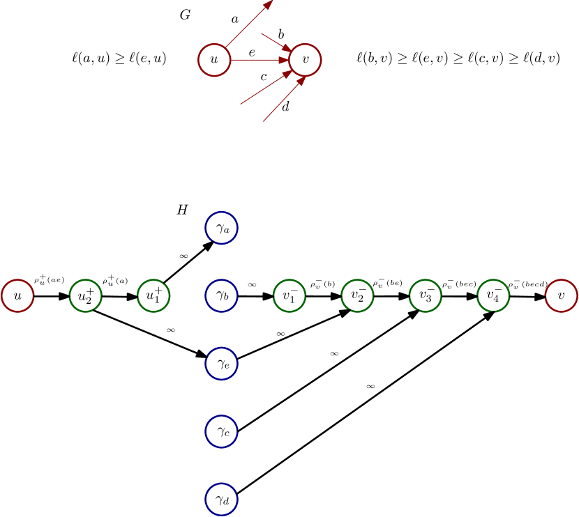
Figure 3: Illustration of the reduction. Only $\delta_{G}^{+}(u)$ and $\delta_{G}^{-}(v)$ shown. The costs on edges in $H$ are shown but not their lengths. The lengths of the infinite cost edges is $0$ and $\ell^{\prime}(u^{+}_{2},u^{+}_{1})=\ell(a,u)-\ell(e,u)$ and $\ell^{\prime}(v_{3}^{-},v_{4}^{-})=\ell(c,v)-\ell(d,v)$.

The graph $H=(V\uplus V^{\prime},E_{H})$ is constructed as follows. To aid the reader we first describe the idea of the construction at a high-level. Consider a node $v\in V$ and the in-coming edges $\delta^{-}(v)$ and out-going edges $\delta^{+}(v)$. In $H$ we have nodes of $V$ and build an in-tree $T^{-}_{v}$ and an out-tree $T^{+}_{v}$ that are rooted at $v$. The leaves of $T^{-}_{v}$ are the edges in $\delta^{-}(v)$ the leaves of $T^{+}_{v}$ are the edges in $\delta^{+}(v)$. Note that an edge $(u,v)$ will thus participate in $T^{+}_{u}$ and $T^{-}_{v}$. Now for the formal details. The nodes of $H$, denoted by $V_{H}$, consist of the nodes $V$ of $G$ and additional nodes $V^{\prime}$. $V^{\prime}$ has two types of nodes. First, for each edge $e\in E$ there is a node $\gamma_{e}$. Second, for each node $v\in V$ we create two sets of nodes $N^{-}(v)$ and $N^{+}(v)$ where $|N^{-}(v)|=n^{-}_{v}=|\delta_{G}^{-}(v)|$ and $|N^{+}(v)|=n^{+}_{v}=|\delta^{+}_{G}(v)|$; thus one node for each edge in $\delta^{-}(v)\cup\delta^{-}(v)$; these will be the internal nodes of the trees $T^{-}_{v}$ and $T^{+}_{v}$ respectively. For notational convenience we refer to the $j$’th node in $N^{-}(v)$ as $v_{j}^{-}$ and similarly $v^{+}_{j}$ for the $j$’th node in $N^{+}(v)$.

Now we describe the edge set $E_{H}$ of the graph $H$, the edge length function $\ell^{\prime}:E_{H}\rightarrow\mathbb{R}_{+}$, and the cost function $c:E_{H}\rightarrow\mathbb{R}_{+}$. The edge set is essentially prescribed by specifying the trees $T^{-}_{v}$ and $T^{+}_{v}$ for each $v\in V$. Consider the vector ${\bf d}^{-}(v)$ of values $\ell(e,v)$ for $e\in\delta_{G}^{-}(v)$. Recall the definition of the Lovász extension $\hat{\rho}^{-}({\bf d}_{v}^{-})$. We order the edges in $\delta^{-}(v)$ as $e_{1},e_{2},\ldots,e_{n_{v}^{-}}$ where $\ell(e_{j},v)\geq\ell(e_{j+1},v)$ for $1\leq j<n_{v}^{-}$ and then $\hat{\rho}^{-}({\bf d}_{v}^{-})=\sum_{j}(\ell(e_{j},v)-\ell(e_{j+1},v))\rho_{v}^{-}(S_{j})$ where $S_{j}=\{e_{1},\ldots,e_{j}\}$. We associate the node $v^{-}_{j}$ with the set $S_{j}$. The edge set of $T^{-}_{v}$ is defined as follows. For ease of notation we let $v^{-}_{n_{v}^{-}+1}$ represent the node $v$. We create a directed path $v_{1}^{-}\rightarrow v_{2}^{-}\rightarrow\ldots\rightarrow v_{n_{v}^{-}}^{-}\rightarrow v_{n_{v}^{-}+1}^{-}=v$ with edge lengths $\ell^{\prime}(v_{1}^{-},v_{2}^{-})=\ell(e_{1},v)-\ell(e_{2},v),\ell^{\prime}(v_{2}^{-},v_{3}^{-})=\ell(e_{2},v)-\ell(e_{3},v),\ldots,\ell^{\prime}(v_{n_{v}^{-}}^{-},v)=\ell(e_{n_{v}^{-}},v)-0$. The costs of these edges are defined as follows: $c(v_{j}^{-},v_{j+1}^{-})=\rho_{v}^{-}(S_{j})$ for $1\leq j\leq n_{v}^{-}$. For each $j$ we add the edge $(\gamma_{e_{j}},v_{j}^{-})$ with length $0$ and cost $\infty$ (for computational purpose a sufficiently large number $M$ would do); this connects the node $\gamma_{e_{j}}$ corresponding to the edge $e_{j}$ to $v_{j}^{-}$ that corresponds to $S_{j}$. See Fig 3.

The construction of $T^{+}_{v}$ is quite similar except that the edge directions are reversed; assuming that the edges in $\delta^{+}(v)$ are ordered such that $\ell(e_{1},v)\geq\ell(e_{2},v)\geq\ldots\geq\ell(e_{n^{+}_{v}},v)$, we create a path $v\rightarrow v^{+}_{n^{+}_{v}}\rightarrow\ldots v^{+}_{2}\rightarrow v^{+}_{1}$ with edge lengths $\ell(e_{n^{+}_{v}},v)-0,\ldots,\ell(e_{j},v)-\ell(e_{j+1},v),\ldots,\ell(e_{1},v)-\ell(e_{2},v)$. The costs for the edges in this path are set to $\rho^{+}_{v}(S_{n_{v}^{+}}),\ldots,\rho_{v}^{+}(S_{1})$ where $S_{j}=\{e_{1},\ldots,e_{j}\}$. For each $j$ we add an edge $(v^{+}_{j},\gamma_{e_{j}})$ with length $0$ and cost $\infty$. This finishes the description of $H$. We now describe various properties of the graph $H$. Several of these properties are staright forward from the description of the construction and we omit proofs of the easy claims.

The proposition below asserts the cost of the fractional solution in the edge-capacitated network $H$ is the same as the cost of the fractional solution in the polymatroidal network $G$.

Proposition 2.

$\sum_{e\in E_{H}}c(e)\cdot\ell^{\prime}(e)=\sum_{v\in V}(\hat{\rho}^{-}({\bf d}^{-}_{v})+\hat{\rho}^{+}({\bf d}^{+}_{v}))$.

Proposition 3.

For any edge $e\in\delta_{G}^{-}(v)$ the length of the unique path in $T_{v}^{-}$ from the node $\gamma_{e}$ to $v$ is equal to $\ell(e,v)$. Similarly for $e\in\delta_{G}^{+}(v)$, the length of the unique path in $T^{+}_{v}$ from the node $v$ to the node $\gamma_{e}$ is equal to $\ell(e,v)$.

We now establish a correspondence between paths in $G$ and $H$ that connect nodes in $V$. Let $e=(u,v)$ be an edge in $G$. We obtain a canonical path $q(u,v)$ from $u$ to $v$ in $H$ as follows: concatenate the unique path from $u$ to $\gamma_{e}$ in $T^{+}_{v}$ with the unique path from $\gamma_{e}$ to $v$ in $T_{v}^{-}$. For any two nodes $s,t\in V$ let $\mathcal{P}_{G}(s,t)$ be the set of (simple) $s$-$t$ paths on $G$ and similarly $\mathcal{P}_{H}(s,t)$ be the paths in $H$. We create a map $g:\mathcal{P}_{G}(s,t)\rightarrow\mathcal{P}_{H}(s,t)$ as follows. Consider a path $p\in\mathcal{P}_{G}(s,t)$; we obtain a path $p^{\prime}\in\mathcal{P}_{H}(s,t)$ corresponding to $p$ as follows. We replace each edge $(u,v)\in p$ by the canonical path $q(u,v)$.

Lemma 4.

The map $g$ is a bijection. Moreover, for any two nodes $u,v\in V$, $\text{dist}_{\ell^{\prime}}(u,v)=\text{dist}_{\ell}(u,v)$.

Now we establish a correspondence between cuts in $G$ and $H$. For a given set of edges $F\subseteq E$ let $\text{sep}_{G}(F)$ be set of node pairs in $V\times V$ separated by $F$ in the graph $G$. Similarly for a set of edges $F^{\prime}\subseteq E_{H}$ let $\text{sep}_{H}(F^{\prime})$ be the set of node pairs in $V\times V$ separated by $F^{\prime}$ in the graph $H$. We say that a set of edges $F$ is minimal with respect to separating node pairs if there is no proper subset of $F$ that separates the same node pairs as $F$.

Proposition 4.

Let $F^{\prime}\subseteq E_{H}$ be minimal with respect to separating node pairs in $V\times V$ and of finite cost. Then for any $v\in V$, $F^{\prime}$ contains at most one edge from $T_{v}^{-}$ and at most one edge from $T_{v}^{+}$.

Proof.

Consider a node $v$ and edge-sets $F^{\prime}\cap T_{v}^{-}$ and $F^{\prime}\cap T_{v}^{+}$. For an edge $e\in E$ there is a node $\gamma_{e}\in V_{H}$ and there is exactly one edge coming into $\gamma_{e}$ and exactly one edge going out of $\gamma_{e}$ and both are of infinite cost. Therefore, if $F^{\prime}$ is of finite cost, $F^{\prime}\cap T_{v}^{-}$ consists of some edges in the path $v_{1}^{-}\rightarrow v_{2}^{-}\ldots\rightarrow v_{n_{v}^{-}}^{-}\rightarrow v$ contained in $T_{v}^{-}$. Since the only way to reach $v$ is through $T_{v}^{-}$ it follows that if $F^{\prime}$ contains an edge $(v_{j}^{-},v^{-}_{j+1})$ then it is redundant to remove an edge $(v_{i}^{-},v_{i+1}^{-})$ for $i<j$. Thus minimality of $F^{\prime}$ implies $F^{\prime}$ contains exactly one edge from $T_{v}^{-}$. The reasoning for $T_{v}^{+}$ is similar. ∎

Lemma 5.

Let $F^{\prime}\subseteq E_{H}$ be minimal with respect to separating node pairs in $V\times V$ and of finite cost. There exists a set of edges $F\subseteq E$ such that $\text{sep}_{G}(F)\supseteq\text{sep}_{H}(F^{\prime})$ and $\nu(F)\leq c(F^{\prime})$.

Proof.

Given a minimal $F^{\prime}$ we obtain a set of edges $F\subseteq E$ as follows. From the proof of Proposition 4 we see that for any node $v$, $F^{\prime}$ contains at most one edge from $T_{v}^{-}$ and in particular if it contains an edge then it is an edge $(v_{j}^{-},v^{-}_{j+1})$ for some $1\leq j\leq n_{v}^{-}$ (for simplicity we identify $v$ with $v^{-}_{n_{v}^{-}+1}$). Suppose there is such an edge $e^{\prime}=(v_{j}^{-},v^{-}_{j+1})$ in $F^{\prime}$. Note that $e^{\prime}$ corresponds to the set $S_{j}=\{e_{1},\ldots,e_{j}\}$ of edges in $\delta_{G}^{-}(v)$ ordered in increasing order by $\ell(e,v)$ values. We add $S_{j}$ to $F$ and assign these edges to $v$ in upper bounding $\nu(F)$: by construction $c(e^{\prime})=\rho_{v}^{-}(S_{j})$. We do a similar procedure if $e^{\prime}\in F\cap T_{v}^{+}$. It follows that the edge set $F$ that we construct satisfies the property that $\nu(F)\leq c(F^{\prime})$.

We now show that $\text{sep}_{G}(F)\supseteq\text{sep}_{H}(F^{\prime})$ Consider a pair $(s,t)$ such that $s$ is separated from $t$ by $F^{\prime}$ in $H$. Suppose $(s,t)$ is not separated by $F$ in $G$. Let $p$ be an $s$-$t$ path that remains in $G\setminus F$. From Proposition 3 there is a unique path $g(p)\in\mathcal{P}_{H}(s,t)$. For every edge $e=(u,v)\in p$ consider the canonical path $q(u,v)$ in $H$. Since $e$ is not in $F$ it implies that $u$ can reach $\gamma_{e}$ in $H\setminus F^{\prime}$ and that $\gamma_{e}$ can reach $v$ in $H\setminus F^{\prime}$. This means that $q(u,v)$ exists in $H\setminus F^{\prime}$. This would imply that $g(p)$ exists in $H\setminus F^{\prime}$ contradicting that assumption that $(s,t)$ is separated by $F^{\prime}$. ∎

We summarize the properties of the reduction. We assume that we have a polymatroidal network $G=(V,E)$ with $k$ demand pairs $(s_{i},t_{i}),\ldots,(s_{k},t_{k})$ with associated demand values $D_{1},\ldots,D_{k}$. For all the cut problems of interest, the relaxations in Section 3 produce a length function $\ell:E\rightarrow\mathbb{R}_{+}$ and for each $e=(u,v)$ associated non-negative values $\ell(e,u)$ and $\ell(e,v)$ such that $\ell(e)=\ell(e,u)+\ell(e,v)$. As before we use ${\bf d}_{v}^{-}$ and ${\bf d}_{v}^{+}$ to denote the vector of $\ell(e,v)$ values for the incoming and outgoing edges at $v$. The reduction produces an edge-capacitated network $H=(V_{H},E_{H})$ with the following properties:

• each node of $V$ is a node in $V_{H}$

• for all $u,v\in V$, $\text{dist}_{\ell}(u,v)=\text{dist}_{\ell^{\prime}}(u,v)$

• $\sum_{e\in E_{H}}c(e)\ell^{\prime}(e)=\sum_{v\in V}(\hat{\rho}_{v}^{-}({\bf d}_{v}^{-})+\hat{\rho}_{v}^{+}({\bf d}_{v}^{+}))$

• for any set of edges $F^{\prime}\subseteq E_{H}$ there is a corresponding set $F\subseteq E$ such that $\text{sep}_{G}(F)\supseteq\text{sep}_{H}(F^{\prime})$ and $\nu(F)\leq c(F^{\prime})$.

We also note that the reduction can be carried out in polynomial time. Moreover, given a set $F^{\prime}\subseteq E_{H}$ a set $F\subseteq E$ that satisfies the last property in the list above can be found in polynomial time.

We build on the reduction to obtain flow-cut gap results, all of which are based on using the relaxations from Section 3 which are dual to the corresponding flow problems. We argue via the reduction and known results on edge-capacitated networks that there exist integral cuts within some factor $\alpha$ of the fractional solution.

4.2 Multicut

We consider the multicut problem for arbitrary demand pairs as well as symmetric demands. The relaxation satisfies the constraint that $\text{dist}_{\ell}(s_{i},t_{i})\geq 1$ for each demand pair $(s_{i},t_{i})$. The reduction from the preceding section produces a graph $H=(V_{H},E_{H})$ and a fractional solution $\ell^{\prime}:E_{H}\rightarrow\mathbb{R}_{+}$ such that $\text{dist}_{\ell^{\prime}}(s_{i},t_{i})\geq 1$. We note that $\ell^{\prime}$ is a feasible solution for the standard distance based relaxation for multicut in edge-capacitated networks which is the dual for the maximum throughput multicommodity flow problem. The integrality gap of this relaxation has been studied and several results are known. Let $\beta=\sum_{e\in E_{H}}c(e)\ell^{\prime}(e)$ be the fractional solution value. Then one can obtain an integral multicut $F^{\prime}$ with cost $c(F^{\prime})$ that can be bounded in terms of $\beta$. We summarize the known results.

• Cheriyan, Karloff and Rabani [8] showed that there exists an $F^{\prime}$ such that $c(F^{\prime})\leq O(1)\cdot\beta^{3}$; this was improved by Gupta [16] to show the existence of a multicut $F^{\prime}$ such that $c(F^{\prime})\leq O(1)\cdot\beta^{2}$. These results hold under the assumption that $c(e)\geq 1$ for all $e$.

• Agrawal, Alon and Charikar [2] improving the results in [8, 16] showed the existence of a cut $F^{\prime}$ such that $c(F^{\prime})=\tilde{O}(n^{11/23})\cdot\beta$. Here $n$ is the number of nodes in the graph.

• Saks, Samorodnitsky and Zosin [34] showed that there exist instances on which every integral multicut has a value $\Omega(k)\cdot\beta$.

• Chuzhoy and Khanna [9] showed that there exist instances on which every multicut has a value $\tilde{\Omega}(n^{1/7})\cdot\beta$. Further, they showed that the multicut problem is hard to approximate to within a factor of $\Omega(2^{\log^{1-\epsilon}n})$ unless $NP\subseteq ZPP$.

Since polymatroidal networks generalize edge-capacitated networks it follows that all the lower bounds in the above hold for the polymatroidal network case as well. The reduction also allows us to obtain upper bound for polymatroidal networks. We have to careful when using bounds that depend on the number of nodes in the graph. The reduction takes $G$ with $n$ nodes and $m$ edges and produces an edge-capacitated graph $H$ with $n+2m$ nodes. In the worst case $H$ has $\Omega(n^{2})$ nodes. We thus obtain the following theorem.

Theorem 1.

In a directed polymatroidal network $G$ on $n$ nodes, for any given multicommodity flow instance with $k$ pairs, if $\beta$ is the maximum throughput multicommodity flow then:

• There is a feasible multicut $F^{\prime}$ such that $\nu(F^{\prime})\leq O(1)\cdot\beta^{2}$ assuming that $\rho^{+}_{v}$ and $\rho_{v}^{-}$ are integer valued for all $v\in V$.

• There is a feasible multicut $F^{\prime}$ such that $\nu(F^{\prime})\leq\tilde{O}(n^{22/23})\cdot\beta$.

Moreover, there exist polynomial-time algorithms to find multicuts guaranteed as above.

Symmetric demands:

We now consider the symmetric demand case when a multicut corresponds to separating $(s_{i},t_{i})$ or $(t_{i},s_{i})$ for a given demand pair $s_{i}t_{i}$. The relaxation for this has a constraint that $\text{dist}_{\ell}(s_{i},t_{i})+\text{dist}_{\ell}(t_{i},s_{i})\geq 1$. In contrast to the strong negative results for the general multicut problem, poly-logarithmic upper bounds on flow-cut gaps are known for symmetric demands in standard networks. In particular Klein et al. [23] show that if $\beta$ is the cost of a fractional solution then there exists an integral multicut of cost $O(\log^{2}k)\cdot\beta$. Even et al. [11] showed the existence of a multicut of cost $O(\log n\log\log n)\cdot\beta$. Note that these bounds are incomparable in that depending on the relationship between $k$ and $n$ one is better than the other. It is also known that there exist instances on which the gap is at least $\Omega(\log n)$. Via the reduction we obtain the following.

Theorem 2.

In a directed polymatroidal network $G$ on $n$ nodes, for any given multicommodity flow instance with symmetric demands on $k$ pairs, the minimum multicut is $O(\min\{\log^{2}k,\log n\log\log n\})\cdot\beta$ where $\beta$ is maximum throughput multicommodity flow for the symmetric demands.

Remark 1.

The flow-cut gap in polymatroidal networks for multiterminal flows can be shown to be $2$ via the reduction and the result of Naor and Zosin [30].

4.3 Sparsest cut

Now we consider the sparsest cut problem where the goal is to find a set of edges $F$ to minimize $\nu(F)/D(F)$ where $D(F)$ is the total demand of the pairs separated by $F$. The relaxation corresponds to finding edge length variables $\ell$ to minimize the fractional cost subject to the constraint that $\sum_{i}D_{i}\cdot\text{dist}_{\ell}(s_{i},t_{i})=1$. Via the reduction we produce an edge-capacitated network $H$ such that $\sum_{i}D_{i}\cdot\text{dist}_{\ell^{\prime}}(s_{i},t_{i})=1$ and with the fractional cost preserved. In edge-capacitated networks there is a generic strategy that translates the flow-cut gap for multicut into a flow-cut gap for sparsest cut at an additional loss of an $O(\log\sum_{i}D_{i})$ factor due to Kahale [19] (see also [37]); this has been refined via a more intricate analysis in [31] to lose only an $O(\log k)$ factor although one needs to apply it carefully. In [2] a simple reduction that loses an $O(\log n)$ factor is given (this builds on [19]). For directed graphs the known-gaps for sparsest cut are essentially based on using the corresponding gap for multicut and translating via the above mentioned schemes. We thus obtain the following results.

Theorem 3.

In a directed polymatroidal network $G$ on $n$ nodes, for any given multicommodity flow instance with $k$ pairs, if $\beta$ is the value of the maximum concurrent flow then there is a cut of sparsity at most $\tilde{O}(n^{22/23})\cdot\beta$.

Theorem 4.

In a directed polymatroidal network $G$ on $n$ nodes, for any given multicommodity flow instance with symmetric demands on $k$ pairs, there is a cut of sparsity $O(\min\{\log^{3}k,\log^{2}n\log\log n\})\cdot\beta$ where $\beta$ is maximum concurrent flow.

5 Flow-Cut Gaps in Undirected Polymatroidal Networks

In this section we consider flow-cut gaps in undirected polymatroidal networks. As we already noted, node-capacitated flows are a special case of polymatroidal flows. We show that line embeddings with low average distortion introduced by Matousek and Rabinovich [29] (and further studied in [32]) are useful for bounding the gap between the maximum concurrent flow and sparsest cut; we are inspired to make this connection from [13] who considered node-capacitated flows. For multicut we show that the region growing technique from [25] that was used in [14] for edge-capacitated multicut can be adapted to the polymatroidal setting. These techniques are also applicable to directed graphs — we defer a more detailed discussion.

5.1 Maximum Concurrent Flow and Sparsest Cut

We start with the definition of line embeddings and average distortion.

Let $(V,d)$ be a finite metric space. A map $g:V\rightarrow\mathbb{R}$ is an embedding of $V$ into a line; it is a contraction (also called $1$-Lipschitz) if for all $u,v\in V$,

$$|g(u)-g(v)|\leq d(u,v).$$

Given a demand function $w:V\times V\rightarrow\mathbb{R}_{+}$ and a contraction $g:V\rightarrow\mathbb{R}$, its average distortion with respect to $w$ is defined as

$$\text{avgd}_{w}(g)=\frac{\sum_{u,v\in V}w(u,v)\cdot d(u,v)}{\sum_{u,v\in V}w(u,v)\cdot|g(u)-g(v)|}$$

The following theorem is implicit in [7]; see [13] for a sketch.

Theorem 5 (Bourgain [7]).

For every $n$-point metric space $(V,d)$ and every weight function $w:V\times V\rightarrow\mathbb{R}_{+}$ there is a polynomial-time computable contraction $g:V\rightarrow\mathbb{R}$ such that $\text{avgd}_{w}(g)=O(\log n)$. Moreover, if the support of $w$ is $k$ there is a map $g$ such that $\text{avgd}_{w}(g)=O(\log k)$.

Using the above we prove the following.

Theorem 6.

In undirected polymatroidal networks, for any given multicommodity flow instance with $k$ pairs, the ratio between the value of the sparsest cut and the value of the maximum concurrent flow is $O(\log k)$. Moreover, there is an efficient algorithm to compute an $O(\log k)$ approximation to the sparsest cut problem.

Recall the relaxation for the sparsest cut from Section 3.3 and the associated notation. To prove the theorem we consider an optimum solution to the relaxation and show the existence of a cut whose sparsity is $O(\log k)$ times the value of the relaxation. Let $(V,d)$ be the metric induced on $V$ by shortest path distances in the graph with edge lengths given by $\ell:E\rightarrow\mathbb{R}_{+}$ from the optimum fractional solution. Let $g:V\rightarrow\mathbb{R}$ be line embedding guaranteed by Theorem 5 with respect to $d$ and the weight function given by the demands $D_{i}$; that is $w(s_{i},t_{i})=D_{i}$ for a demand pair and is $0$ for any pair of nodes that do not correspond to a demand. Without loss of generality we can assume that $g$ maps $V$ to the interval $[0,\beta]$ for some $\beta>0$. For $\theta\in(0,\beta)$ let $S_{\theta}=\{u\mid g(u)\leq\theta\}$. We show that there is a $\theta$ such that $\delta(S_{\theta})$ is an approximately good sparse cut. Let $D(\delta(S_{\theta}))$ be the total demand of pairs separated by $S_{\theta}$, that is $D(\delta(S_{\theta}))=\sum_{i:S_{\theta}\text{~{}separates~{}}s_{i}t_{i}}D_{i}$.

Lemma 6.

$$\int_{0}^{\beta}D(\delta(S_{\theta}))d\theta=\Omega\left(\frac{1}{\log k}\right).$$

Proof.

From the definition of $D(\delta(S_{\theta}))$,

$$\int_{0}^{\beta}D(\delta(S_{\theta}))d\theta=\int_{0}^{\beta}(\sum_{i:S_{\theta}\text{~{}separates~{}}s_{i}t_{i}}D_{i})d\theta=\sum_{i=1}^{k}D_{i}\cdot\int_{0}^{\beta}{\bf 1}_{S_{\theta}\text{~{}separates~{}}s_{i}t_{i}}d\theta=\sum_{i=1}^{k}D_{i}\cdot|g(s_{i})-g(t_{i})|.$$

From the properties of $g$,

$$\frac{\sum_{i}D_{i}\cdot d(s_{i},t_{i})}{\sum_{i}D_{i}\cdot|g(s_{i})-g(t_{i})|}\leq O(\log k).$$

We have the constraint $\sum_{i}D_{i}\cdot d(s_{i},t_{i})=1$ from the LP relaxation; this combined with the above inequality proves the lemma. ∎

The main insight in the proof is the following lemma. A version of the lemma also holds for directed graphs that we address in a remark following the proof.

Lemma 7.

$$\int_{0}^{\beta}\nu(\delta(S_{\theta}))d\theta\leq 2\sum_{u}\hat{\rho}_{u}({\bf d}_{u}).$$

Proof.

Consider an edge $uv\in\delta(S_{\theta})$ and for simplicity assume $g(u)<g(v)$. The length of $e$ in the embedding is $\ell^{\prime}(e)=|g(v)-g(u)|\leq\ell(e)$. The edge $(u,v)\in\delta(S_{\theta})$ iff $\theta$ is in the interval $[g(u),g(v)]$. Note that the cost $\nu(\delta(S_{\theta}))$ is in general a complicated function to evaluate. We upper bound $\nu(\delta(S_{\theta}))$ by giving an explicit way to assign $e=uv$ to either $u$ or $v$ as follows. Recall that in the relaxation $\ell(e)=\ell(e,u)+\ell(e,v)$ where $\ell(e,u)$ and $\ell(e,v)$ are the contributions of $u$ and $v$ to $e$. Let $r=\frac{\ell(e,u)}{\ell(e)}$ and let $\ell^{\prime}(e,u)=r\ell^{\prime}(e)$ and $\ell^{\prime}(e,v)=(1-r)\ell^{\prime}(e)$. We partition the interval $[g(u),g(v)]$ into $[g(u),g(u)+\ell^{\prime}(e,u))$ and $[g(u)+\ell^{\prime}(e,u),g(v)]$; if $\theta$ lies in the former interval we assign $e$ to $u$, otherwise we assign $e$ to $v$. This assignment procedures describes a way to upper bound $\nu(\delta(S_{\theta}))$ for each $\theta$. Now we consider the quantity $\int_{0}^{\beta}\nu(\delta(S_{\theta}))d\theta$ and upper bound it as follows.

Consider a node $u$ and let $L_{u}=\{uv\in\delta(u)\mid g(v)<g(u)\}$ be the set of edges $uv$ that go from $u$ to the left of $u$ in the embedding $g$. Similarly $R_{u}=\{uv\in\delta(u)\mid g(v)\geq g(u)\}$. Note that $L_{u}$ and $R_{u}$ partition $\delta(u)$. Let ${\bf d}^{\prime}_{u}$ be the vector of dimension $|\delta(u)|$ consisting of the values $\ell^{\prime}(e,u)$ for $e\in\delta(u)$. We obtain ${\bf d}^{L}_{u}$ from ${\bf d}^{\prime}_{u}$ by setting the values for $e\in R_{u}$ to $0$ and similarly ${\bf d}^{R}_{u}$ from ${\bf d}^{\prime}_{u}$ by setting the values for $e\in L_{u}$ to $0$. Since $0\leq\ell^{\prime}(e,u)\leq\ell(e,u)$ for each $e\in\delta(u)$ we see that ${\bf d}^{\prime}_{u}\leq{\bf d}_{u}$ and (component wise) and hence ${\bf d}^{L}_{u}\leq{\bf d}_{u}$ and ${\bf d}^{R}_{u}\leq{\bf d}_{u}$. Since $\rho_{u}$ is monotone we have that $\hat{\rho}_{u}({\bf d}^{L}_{u})\leq\hat{\rho}_{u}({\bf d}_{u})$ and $\hat{\rho}_{u}({\bf d}^{R}_{u})\leq\hat{\rho}_{u}({\bf d}_{u})$ (see Proposition 1).

We claim that

$$\int_{0}^{\beta}\nu(\delta(S_{\theta}))d\theta\leq\sum_{u\in V}(\hat{\rho}_{u}({\bf d}^{L}_{u})+\hat{\rho}_{u}({\bf d}^{R}_{u})),$$

which would prove the lemma.

To see the claim consider some fixed $\theta$ and $\nu(\delta(S_{\theta}))$. Fix a node $u$ and consider the edges in $\delta(u)\cap S_{\theta}$ assigned to $u$ by the procedure we described above; call this set $A_{\theta,u}$. First assume that $\theta<g(u)$. Then the edges assigned to $u$ by the procedure, denoted by $A_{\theta,u}=\{e\in L_{u}\mid\theta>g(u)-\ell^{\prime}(e,u)\}$. Similarly, if $\theta>g(u)$, $A_{\theta,u}=\{e\in L_{u}\mid\theta<g(u)+\ell^{\prime}(e,u)\}$. From these definitions we have

$$\int_{0}^{\beta}\nu(\delta(S_{\theta}))d\theta\leq\sum_{u\in V}\int_{0}^{\beta}\rho_{u}(A_{\theta,u})d\theta.$$

For a fixed node $u$,

$$\int_{0}^{\beta}\rho_{u}(A_{\theta,u})d\theta = \int_{0}^{g(u)}\rho_{u}(A_{\theta,u})d\theta+\int_{g(u)}^{\beta}\rho_{u}(A_{\theta,u})d\theta$$

Let $L_{u}=\{e_{1},e_{2},\ldots,e_{h}\}$ where $0\leq\ell^{\prime}(e_{1},u)\leq\ell^{\prime}(e_{2},u)\leq\ldots\leq\ell^{\prime}(e_{h},u)$. Then

$$\int_{0}^{g(u)}\rho_{u}(A_{\theta,u})d\theta=\sum_{j=1}^{h}(\ell^{\prime}(e_{j},u)-\ell^{\prime}(e_{j-1},u))\rho(\{e_{1},e_{2},\ldots,e_{j}\})$$

The right hand side of the above, is by construction and the definition of the Lovász extension, equal to $\hat{\rho}_{u}({\bf d}^{L}_{u})$. Similarly, $\int_{g(u)}^{\beta}\rho_{u}(A_{\theta,u})d\theta=\hat{\rho}_{u}({\bf d}^{R}_{u})$. ∎

Remark 2.

An examination of the proof of the above lemma explains the factor of $2$ on the right hand side; the edges in $\delta(v)$ can be both to the left and right of $v$ in the line embedding and each side contributes $\hat{\rho}_{u}({\bf d}_{v})$ to the cost. This is related to the technical issue about undirected polymatroid networks where the flow through $v$ takes up capacity on two edges incident to $v$. For directed graphs one can prove a statement of the form below where $\delta^{+}(S_{\theta})$ is set of edges leaving $S_{\theta}$. Notice that there is no factor of $2$ since one treats the incoming and outgoing edges separately.

$$\int_{0}^{\beta}\nu(\delta^{+}(S_{\theta}))d\theta\leq\sum_{u}(\hat{\rho}_{u}^{-}({\bf d}^{-}_{u})+\hat{\rho}_{u}^{+}({\bf d}^{+}_{u})).$$

The above statement gives an embedding proof of the maxflow-mincut theorem for single-commodity directed polymatroidal networks and has other applications.

We now finish the proof of Theorem 6 via the preceding two lemmas.

$$\min_{\theta\in(0,\beta)}\frac{\nu(\delta(S_{\theta}))}{D(\delta(S_{\theta}))} \leq \frac{\int_{0}^{\beta}\nu(\delta(S_{\theta}))d\theta}{\int_{0}^{\beta}D(\delta(S_{\theta}))d\theta}$$

$$\leq 2\sum_{u}\hat{\rho}_{u}({\bf d}_{u})\cdot O(\log k)=O(\log k)\sum_{u}\hat{\rho}_{u}({\bf d}_{u}).$$

The above shows that the sparsity of $S_{\theta}$ for some $\theta$ is at most $O(\log k)$ times $\sum_{u}\hat{\rho}_{u}({\bf d}_{u})$ which is the value of the relaxation. Given a line embedding $g$ there are only $n-1$ distinct cuts of interest and one can try all of them to find the one with the smallest sparsity. The efficiency of the algorithm therefore rests on the efficiency of the algorithm to solve the fractional relaxation, and the algorithm to find a line embedding guaranteed by Theorem 5; both have polynomial time algorithms and thus one can find an $O(\log k)$ approximation to the sparsest cut in polynomial time.

Remark 3.

Node-weighted flows and cuts/separators can be cast as special cases of flows and cuts in polymatroid networks. Our algorithm produces edge-cuts from line embeddings in a simple way even for node-weighted problems — the $\nu$ cost of the edge-cut automatically translates into an appropriate node-weighted cut. In contrast, the algorithm in [13] has to solve several instances of $s$-$t$ separator problems in auxiliary graphs obtained from the line embedding.

5.1.1 Sparsest Bi-partition Cut

We worked with general edge cuts so far, but for certain applications, it is necessary to work with a special type of edge cut called a bi-partition cut. In an undirected polymatroidal network, an edge-cut $F$ is said to be a bi-partition cut if there exists a set $S\subseteq V$ such that $F=\delta_{G}(S)$. In the case of edge-capacitated undirected networks, it is well known that for any multicommodity flow instance, there always exists a sparsest cut that is a bi-partition cut. This does not hold for polymatroidal networks, however, a factor $2$ gap can indeed be shown between the sparsest cut and the sparsest cut restricted to bi-partition cuts; moreover this factor is tight.

Theorem 7.

Given any edge cut $F$ for a multicommodity flow instance in an undirected polymatroidal network $G=(V,E)$, there exists a bi-partition cut $\delta_{G}(S)$ whose sparsity is atmost $2$ times the sparsity of $F$. Furthermore this factor is tight.

The proof of the above theorem can be found in Section C of the appendix. Theorem 6 and Theorem. 7 together imply a logarithmic gap between maximum concurrent flow and sparsest bi-partition cut. This is formally stated in the following corollary.

Corollary 1.

In undirected polymatroidal networks, for any given multicommodity flow instance with $k$ pairs, the ratio between the value of the sparsest bi-partition cut and the value of the maximum concurrent flow is $O(\log k)$.

5.2 Maximum Throughput Flow and Multicut

We prove the following theorem in this section.

Theorem 8.

In undirected polymatroidal networks, for any given multicommodity flow instance with $k$ pairs, the ratio between the value of the minimum multicut and the value of the maximum throughput flow is $O(\log k)$. Moreover, there is an efficient algorithm to compute an $O(\log k)$ approximation to the minimum multicut problem.

We recall the relaxation for the minimum mulitcut problem from Section 3.2. Consider an optimum solution to the relaxation given by edge lengths $\ell(e),e\in E$ and the partition of $\ell(e)$ for each $e=uv$ between $u$ and $v$ given by the variables $\ell(e,u)$ and $\ell(e,v)$. We will show that there exists a multicut $F\subseteq E$ for the given pairs such that $\nu(F)=O(\log k)(\sum_{v}\hat{\rho}_{v}({\bf d}_{v}))$.

By slightly generalizing the proof of Lemma 7 we obtain the following.

Lemma 8.

Let $g:V\rightarrow[0,\beta]$ be a contraction, let $0\leq a_{0}\leq a<b\leq b_{0}\leq\beta$ and $S_{\theta}=\{u\mid g(u)<\theta\}$. Suppose for every edge $e=uv\in\cup_{\theta\in[a,b]}\delta(S_{\theta})$, $g(u)$ and $g(v)$ are both in $[a_{0},b_{0}]$. Then,

$$\int_{a}^{b}\nu(\delta(S_{\theta}))d\theta\leq 2\sum_{v:g(v)\in[a_{0},b_{0}]}\hat{\rho}_{v}({\bf d}_{v}).$$

Proof.

The proof is very similar to the proof of Lemma 7, except that to upper bound the left hand side in the statement of the lemma, we only need to consider edges that are in the set $\cup_{\theta\in[a,b]}\delta(S_{\theta})$. The condition in the lemma assures us that any node that is involved in $\delta(S_{\theta})$ have to lie within the interval $[a_{0},b_{0}]$. Thus, it is sufficient to consider the set of nodes $v:g(v)\in[a_{0},b_{0}]$ in the integral on the right hand side. The proof is written out in detail in Sec. B. ∎

Given a graph $G$ with edge lengths $\ell:E\rightarrow\mathbb{R}_{+}$, a node $v$ and radius $r$, let $B^{\ell}_{G}(v,r)=\{u\mid\text{dist}_{\ell}(v,u)\leq r\}$ denote the ball of radius $r$ around $v$ according to edge lengths $\ell$. We omit $\ell$ and $G$ if they are clear from the context. For a set of nodes $X\subseteq V$ we let $\text{{\rm vol}}(X)=\sum_{v\in X}\hat{\rho}_{v}({\bf d}_{v})$ denote the total contribution of the nodes in $X$ to the objective function.

Lemma 9.

Let $\delta<1$ and suppose $\ell(e)<\frac{\delta}{2\log k}$ for all $e$. Then, for any given node $s$ and $k\geq 2$ there exists a $r\in[0,\delta)$ such that $\nu(\delta(B(s,r))\leq a\log k\cdot\frac{1}{\delta}(\text{{\rm vol}}(B(s,r))+\text{{\rm vol}}(V)/k)$, with $a=28$.

Proof.

For simplicity we assume here that $\log k$ is an integer multiple of $3$. Order the nodes in increasing order of distance from $s$: this produces a line embedding $g_{s}:V\rightarrow\mathbb{R}_{+}$. For integer $i\geq 0$ define $r_{i}=\frac{i\cdot\delta}{2\log k}$. Define $\alpha_{0}=\text{{\rm vol}}(V)/k$ and for $i\geq 1$ let $\alpha_{i}=\alpha_{0}+\text{{\rm vol}}(B(s,r_{i}))$.

Consider any $1\leq j\leq 2\log k$. We apply Lemma 8 to the embedding $g_{s}$ and the interval $[r_{j-1},r_{j}]$; note that $\ell(e)<\frac{\delta}{2\log k}$ which implies that we can indeed apply the lemma. Also any edge $e\in\cup_{\theta\in[r_{j-1},r_{j}]}\delta(S_{\theta})$ satisfies the property that $g(u)\in[r_{j-2},r_{j+1}]$ and $g(v)\in[r_{j-2},r_{j+1}]$ since $\ell(e)<\frac{\delta}{2\log k}$. Thus

$$\int_{r_{j-1}}^{r_{j}}\nu(\delta(B(s,\theta))d\theta \leq 2\sum_{v:g_{s}(v)\in[r_{j-2},r_{j+1}]}\hat{\rho}_{v}({\bf d}_{v})$$ (5)

$$\leq 2(\alpha_{j+1}-\alpha_{j-2})$$

We claim that there is some $1\leq j<2\log k$ such that $\alpha_{j+1}\leq 8\alpha_{j-2}$. Suppose not, then $\alpha_{3i}>8\alpha_{3(i-1)}$ for all $1\leq i\leq\frac{2\log k}{3}$. This implies that $\alpha_{3i}>8^{i}\alpha_{0}=2^{3i}\alpha_{0}$. Therefore, with $i=\frac{2\log k}{3}$, this implies that $\alpha_{2\log k}>2^{2\log k}\frac{\text{{\rm vol}}(V)}{k}>4\text{{\rm vol}}(V)$ which is impossible.

Thus there exists a $j$ such that $\alpha_{j+1}\leq 8\alpha_{j-2}$. Consider that $j$, equation (5) implies that

$$\int_{r_{j-1}}^{r_{j}}\nu(\delta(B(s,\theta))d\theta \leq 2(\alpha_{j+1}-\alpha_{j-2})$$

$$\leq 2(7\alpha_{j-2}).$$

If we pick $r$ uniformly at random from the interval $[r_{j-1},r_{j}]$, where satisfies the above property, the expected cost of $\nu(\delta(B(s,r)))$ is

$$\frac{1}{r_{j}-r_{j-1}}\int_{r_{j-1}}^{r_{j}}\nu(\delta(B(s,\theta))d\theta\leq\frac{28\log k}{\delta}\alpha_{j-2},$$

from the preceding inequality and the fact that $r_{j}-r_{j-1}=\frac{\delta}{2\log k}$. Hence there exists an $r\in[r_{j-1},r_{j}]$ such that $\nu(\delta(B(s,r)))\leq\frac{28\log k}{\delta}\alpha_{j-2}$. Since $\alpha_{j-2}-\alpha_{0}\leq\text{{\rm vol}}(B(s,r))$, the lemma follows. ∎

Now we consider the following algorithm for finding a multicut from a given fractional solution.

• Let $F\leftarrow\{e\mid\ell(e)\geq\frac{1}{4\log k}\}$.

• $G^{\prime}\leftarrow G[E\setminus F]$.

• While (there exists a pair $s_{i}t_{i}$ connected in $G^{\prime}$) do

  • Let $s_{j}t_{j}$ be a pair connected in $G^{\prime}$.

  • Via Lemma 9 with $\delta=1/2$ find $r<1/2$ such that $\nu(\delta_{G^{\prime}}(B_{G^{\prime}}(s_{j},r)))\leq 2a\log k\cdot(\text{{\rm vol}}(B_{G^{\prime}}(s_{j},r))+\text{{\rm vol}}(V)/k)$.

  • $F\leftarrow F\cup\delta_{G^{\prime}}(B_{G^{\prime}}(s_{j},r))$.

  • Remove the vertices $B_{G^{\prime}}(s_{j},r)$ and edges incident to them from $G^{\prime}$.

• Output $F$ as the multicut.

Lemma 10.

The set of edges $F$ output by the algorithm is a feasible multicut for the given instance.

Proof.

(Sketch) One can prove this by induction on the number of steps in the while loop. We consider the first step. The diameter of the ball $B_{G^{\prime}}(s_{j},r)$ is $2r<1$ and hence the end points of any pair cannot both be inside this ball. We remove the edges $\delta(B_{G^{\prime}}(s_{j},r))$ and by the preceding observation there is no need to recurse on this ball. The algorithm recurses on the remaining graph $G^{\prime}-B_{G^{\prime}}(s_{j},r)$, and by induction separates any pair with both end points in that graph. ∎

Now we argue about the cost of the set $F$ output by the algorithm. Let $F_{0}\leftarrow\{e\mid\ell(e)\geq\frac{1}{4\log k}\}$ be the initial set of edges added to $F$ and let $F_{i}$ be the set of edges added in the $i$’th iteration of the while loop.

Lemma 11.

$\nu(F_{0})\leq 8\log k\cdot\sum_{v}\hat{\rho}_{v}({\bf d}_{v})$.

Proof.

For $v\in V$ let $A_{v}=\{e\in\delta(v)\cap F_{0}\mid\ell(e,v)\geq\frac{1}{8\log k}\}$. We can upper bound $\nu(F_{0})$ by $\sum_{v}\rho_{v}(A_{v})$ since the latter term counts each edge $uv\in F_{0}$ in at least one of $A_{u}$ and $A_{v}$ since $\ell(e,u)+\ell(e,v)=\ell(e)\geq\frac{1}{4\log k}$. From the definition of the Lovász extension

$$\hat{\rho}_{v}({\bf d}_{v})=\int_{0}^{1}\rho_{v}({\bf d}_{v}^{\theta})d\theta\geq\int_{0}^{1/(8\log k)}\rho_{v}({\bf d}_{v}^{\theta})d\theta\geq\frac{1}{8\log k}\rho_{v}(A_{v}),$$

where we used non-negativity of $\rho_{v}$ for the first inequality above and monotonicity for the second. ∎

Lemma 12.

$\sum_{i\geq 1}\nu(F_{i})\leq 4a\log k\sum_{v}\hat{\rho}_{v}({\bf d}_{v})$.

Proof.

(Sketch) From the algorithm description, $F_{i}=\delta(B_{G^{\prime}}(s_{j},r))$ for some terminal $s_{j}$ and radius $r<1/2$ where $G^{\prime}$ is the remaining graph in iteration $i$. Moreover, $\nu(F_{i})\leq 2a\log k\cdot(\text{{\rm vol}}(B_{G^{\prime}}(s_{j},r))+\text{{\rm vol}}(V)/k)$. Since the nodes in $B_{G^{\prime}}(s_{j},r)$ are removed from the graph, a node $u$ is charged only once inside a ball. Hence

$$\sum_{i}\nu(F_{i})\leq\sum_{i}2a\log k\cdot\text{{\rm vol}}(V)/k+2a\log k\sum_{v}\hat{\rho}_{v}({\bf d}_{v})\leq 4a\log k\sum_{v}\hat{\rho}_{v}({\bf d}_{v}),$$

since there are at most $k$ iterations of the while loop; each iteration separates at least one pair. ∎

Since $\nu$ is subadditive (see Lemma 1)

$$\nu(F)\leq\nu(F_{0})+\sum_{i\geq 1}\nu(F_{i})\leq(8+4a)\log k\sum_{v}\hat{\rho}_{v}({\bf d}_{v}).$$

This finishes the proof of Theorem 8.

6 Conclusions

We considered multicommodity flows and cuts in polymatroidal networks and derived flow-cut gap results in several settings. These results generalize some existing results for the well-studied edge and node-capacitated networks. We briefly mention two results that can be obtained via the line embeddings technique that we did not include in this paper. A multicommodity flow instance in an undirected network $G=(V,E)$ is a product multicommodity flow instance if there there is a non-negative weight function $\pi:V\rightarrow\mathbb{R}_{+}$ and the demand $D_{uv}$ between $u$ and $v$ is $\pi(u)\cdot\pi(v)$. The associated cut problem is interesting because it corresponds to finding sparse separators in graphs which in turn can be used to find balanced separators; these have several applications. It was shown in [22] that in edge-capacitated undirected planar networks, the flow-cut gap for product multicommodity flow instances is $O(1)$ (in fact they showed this holds for any class of graphs that excludes a fixed graph as a minor). Rabinovich [32] showed that the main technical theorem in [22] also leads to a line embedding theorem, and this was used in [13] to show an $O(1)$ flow-cut gap for product multicommodity flow instances in node-capacitated planar graphs. Our work here shows that this is true for undirected planar polymatroidal networks. Arora, Rao and Vazirani [4] gave an $O(\sqrt{\log n})$-approximation, via a semi-definite programming relaxation, for the sparsest cut problem in an undirected edge-capacitated network. Note that this is not a traditional flow-cut gap result since the SDP-based relaxation used is strictly stronger than the dual of the multicommodity flow relaxation. By interpreting the main technical result in [4] as a line-embedding theorem, [13] obtained an $O(\sqrt{\log n})$-approximation for sparsest cut in node-capacitated graphs; this can also be extended to the polymatroidal setting.

Flow-cut gap questions for node-capacitated problems are less well-understood than the corresponding questions for edge-capacitated problems; line-embeddings provide a tool to obtain upper bounds on the gap but they do not provide a tight characterization as $\ell_{1}$-embeddings do for the edge-capacitated case. We hope that polymatroidal networks and their applications to network information flow provide a new impetus for understanding these questions.

Appendix A Proof of Lemma 13

Lemma 13.

For a directed polymatroidal network, the dual of the maximum throughput flow problem is equivalent (in terms of value) to the program given by (3) (for undirected the program given by (4)).

Proof.

We will show the proof for the undirected case, the proof for the directed case is similar. The program for maximum throughput flow is given by:

$$\max\quad\sum_{i}\sum_{p\in\mathcal{P}_{(s_{i},t_{i})}}f(p)$$

s.t.

$$\sum_{{e}:{e}\in S}\sum_{p:{e}\in p}f(p) \leq \rho_{v}(S)\quad\forall S\subseteq\delta(v)\ \forall v\in V$$

$$f(p) \geq 0\quad\forall p\in\mathcal{P}_{\left(s_{i},t_{i}\right)},\forall i=1\ldots k.$$

The dual of the flow linear program can now be written. Let the dual variables $d_{v}(S_{v})$ correspond to the non-trivial constraint in the above linear program. Then the dual linear program is:

$$\mathcal{P}_{d}:=\min\quad\sum_{v\in V}\sum_{S\subseteq\delta(v)}d_{v}(S)\rho_{v}(S)$$

s.t.

$$\sum_{e=uv:e\in p}\left(\sum_{S\subseteq\delta(u):e\in S}d_{u}(S)+\sum_{S\subseteq\delta(v):e\in S}d_{v}(S)\right) \geq 1\quad\forall p\in\mathcal{P}_{(s_{i},t_{i})}\text{ where }\ \ e=uv$$

$$d_{u}(S) \geq 0\ \forall u\in V\ \forall S\subseteq\delta(u).$$

This can be rewritten equivalently as

$$\mathcal{P}_{d} := \min\quad\sum_{v\in V}\sum_{S\subseteq\delta(v)}d_{v}(S)\rho_{v}(S)$$

s.t.

$$\ell(e) := \left(\sum_{S\subseteq\delta(u):e\in S}d_{u}(S)+\sum_{S\subseteq\delta(v):e\in S}d_{v}(S)\right)$$

$$\text{dist}_{\ell}(s_{i},t_{i}) \geq 1\quad 1\leq i\leq k$$

$$d_{u}(S) \geq 0\ \forall u\in V\ \forall S\subseteq\delta(u).$$

Let us define new variables $\ell(e,u)$, $\ell(e,v)$ for each edge $e=uv$, and rewrite the linear program:

$$\min\quad\sum_{v\in V}\sum_{S\subseteq\delta(v)}d_{v}(S)\rho_{v}(S)$$

s.t.

$$\ell(e) := \ell(e,u)+\ell(e,v),\text{ where }\ e=uv$$

$$\ell(e,u) = \sum_{S\subseteq\delta(u):e\in S}d_{u}(S)\ \forall e\in E,e=uv$$

$$\ell(e,v) = \sum_{S\subseteq\delta(v):e\in S}d_{v}(S)\quad\forall e\in E,e=uv$$

$$\text{dist}_{\ell}(s_{i},t_{i}) \geq 1\quad 1\leq i\leq k$$

$$d_{u}(S) \geq 0$$

$$\ell(e,u),\ell(e,v) \geq 0\quad\forall u\in V\ \forall S\subseteq\delta(u).$$

The minimization is over the variables $\ell(e,u)$ and $d_{v}(S)$. Observe for any fixed $v$ the variables $d_{v}(S),S\subseteq\delta(v)$ influence only the variable $\ell(e,v),e\in\delta(v)$. Hence, for any $v$ and a fixed assignment set of values $\ell(e,v),e\in\delta(v)$ the optimal choice of variables $d_{v}(S),S\subseteq\delta(v)$ can be obtained by solving the following linear program:

$$\min\quad\sum_{S\subseteq\delta(v)}d_{v}(S)\rho_{v}(S)$$

s.t.

$$\sum_{S\subseteq\delta(v):e\in S}d_{v}(S) = \ell(e,v)\quad\forall e\in E,e=uv$$

$$d_{u}(S) \geq 0,\quad S\subseteq\delta(v),\ \forall v\in V.$$

Recalling the definition of the convex closure of a function, one sees that the value of the above linear program is equal to $\tilde{\rho}_{v}({\bf d}_{v})$; note that for polymatroids we can drop the constraint $\sum_{S}d_{v}(S)=1$ in the linear program for the convex closure. Since the convex closure is equval to the Lovász extension we obtain the desired equivalence of the formulations. ∎

Appendix B Proof of Lemma 8

Lemma 14.

Let $g:V\rightarrow[0,\beta]$ be a contraction, let $0\leq a_{0}\leq a<b\leq b_{0}\leq\beta$ and $S_{\theta}=\{u\mid g(u)<\theta\}$. Suppose for every edge $e=uv\in\cup_{\theta\in[a,b]}\delta(S_{\theta})$, $g(u)$ and $g(v)$ are both in $[a_{0},b_{0}]$. Then,

$$\int_{a}^{b}\nu(\delta(S_{\theta}))d\theta\leq 2\sum_{v:g(v)\in[a_{0},b_{0}]}\hat{\rho}_{v}({\bf d}_{v}).$$

Proof.

Consider an edge $uv\in\delta(S_{\theta})$ and for simplicity assume $g(u)<g(v)$. The length of $e$ in the embedding is $\ell^{\prime}(e)=|g(v)-g(u)|\leq\ell(e)$. The edge $(u,v)\in\delta(S_{\theta})$ iff $\theta$ is in the interval $[g(u),g(v)]$. Also by the conditions of the theory for every such $(u,v)$, $g(u)\in[a_{0},b_{0}]$ and $g(v)\in[a_{0},b_{0}]$. Note that the cost $\nu(\delta(S_{\theta}))$ is in general a complicated function to evaluate. We upper bound $\nu(\delta(S_{\theta}))$ by giving an explicit way to assign $e=uv$ to either $u$ or $v$ as follows. Recall that in the relaxation $\ell(e)=\ell(e,u)+\ell(e,v)$ where $\ell(e,u)$ and $\ell(e,v)$ are the contributions of $u$ and $v$ to $e$. Let $r=\frac{\ell(e,u)}{\ell(e)}$ and let $\ell^{\prime}(e,u)=r\ell^{\prime}(e)$ and $\ell^{\prime}(e,v)=(1-r)\ell^{\prime}(e)$. We partition the interval $[g(u),g(v)]$ into $[g(u),g(u)+\ell^{\prime}(e,u))$ and $[g(u)+\ell^{\prime}(e,u),g(v)]$; if $\theta$ lies in the former interval we assign $e$ to $u$, otherwise we assign $e$ to $v$. This assignment procedures describes a way to upper bound $\nu(\delta(S_{\theta}))$ for each $\theta$. Now we consider the quantity $\int_{a}^{b}\nu(\delta(S_{\theta}))d\theta$ and upper bound it as follows.

Consider a node $u$ and let $L_{u}=\{uv\in\delta(u)\mid g(v)<g(u)\}$ be the set of edges $uv$ that go from $u$ to the left of $u$ in the embedding $g$. Similarly $R_{u}=\{uv\in\delta(u)\mid g(v)\geq g(u)\}$. Note that $L_{u}$ and $R_{u}$ partition $\delta(u)$. Let ${\bf d}^{\prime}_{u}$ be the vector of dimension $|\delta(u)|$ consisting of the values $\ell^{\prime}(e,u)$ for $e\in\delta(u)$. We obtain ${\bf d}^{L}_{u}$ from ${\bf d}^{\prime}_{u}$ by setting the values for $e\in R_{u}$ to $0$ and similarly ${\bf d}^{R}_{u}$ from ${\bf d}^{\prime}_{u}$ by setting the values for $e\in L_{u}$ to $0$. Since $0\leq\ell^{\prime}(e,u)\leq\ell(e,u)$ for each $e\in\delta(u)$ we see that ${\bf d}^{\prime}_{u}\leq{\bf d}_{u}$ and (component wise) and hence ${\bf d}^{L}_{u}\leq{\bf d}_{u}$ and ${\bf d}^{R}_{u}\leq{\bf d}_{u}$. Since $\rho_{u}$ is monotone we have that $\hat{\rho}_{u}({\bf d}^{L}_{u})\leq\hat{\rho}_{u}({\bf d}_{u})$ and $\hat{\rho}_{u}({\bf d}^{R}_{u})\leq\hat{\rho}_{u}({\bf d}_{u})$ (see Proposition 1).

We claim that

$$\int_{a}^{b}\nu(\delta(S_{\theta}))d\theta\leq\sum_{u\in V:g(u)\in[a_{0},b_{0}]}(\hat{\rho}_{u}({\bf d}^{L}_{u})+\hat{\rho}_{u}({\bf d}^{R}_{u})),$$

which would prove the lemma.

To see the claim consider some fixed $\theta$ and $\nu(\delta(S_{\theta}))$. Fix a node $u$ and consider the edges in $\delta(u)\cap S_{\theta}$ assigned to $u$ by the procedure we described above; call this set $A_{\theta,u}$. First assume that $\theta<g(u)$. Then the edges assigned to $u$ by the procedure, denoted by $A_{\theta,u}=\{e\in L_{u}\mid\theta>g(u)-\ell^{\prime}(e,u)\}$. Similarly, if $\theta>g(u)$, $A_{\theta,u}=\{e\in L_{u}\mid\theta<g(u)+\ell^{\prime}(e,u)\}$. From these definitions we have

$$\nu(\delta(S_{\theta})) \leq \sum_{u\in V:g(u)\in[a_{0},b_{0}]}\rho_{u}(A_{\theta,u})$$

$$\Rightarrow\int_{a}^{b}\nu(\delta(S_{\theta}))d\theta \leq \sum_{u\in V:g(u)\in[a_{0},b_{0}]}\int_{a}^{b}\rho_{u}(A_{\theta,u})d\theta$$

$$\leq \sum_{u\in V:g(u)\in[a_{0},b_{0}]}\int_{0}^{\beta}\rho_{u}(A_{\theta,u})d\theta.$$

For a fixed node $u$,

$$\int_{0}^{\beta}\rho_{u}(A_{\theta,u})d\theta = \int_{0}^{g(u)}\rho_{u}(A_{\theta,u})d\theta+\int_{g(u)}^{\beta}\rho_{u}(A_{\theta,u})d\theta$$

Let $L_{u}=\{e_{1},e_{2},\ldots,e_{h}\}$ where $0\leq\ell^{\prime}(e_{1},u)\leq\ell^{\prime}(e_{2},u)\leq\ldots\leq\ell^{\prime}(e_{h},u)$. Then

$$\int_{a}^{g(u)}\rho_{u}(A_{\theta,u})d\theta=\sum_{j=1}^{h}(\ell^{\prime}(e_{j},u)-\ell^{\prime}(e_{j-1},u))\rho(\{e_{1},e_{2},\ldots,e_{j}\})$$

The right hand side of the above, is by construction and the definition of the Lovász extension, equal to $\hat{\rho}_{u}({\bf d}^{L}_{u})$. Similarly, $\int_{g(u)}^{\beta}\rho_{u}(A_{\theta,u})d\theta=\hat{\rho}_{u}({\bf d}^{R}_{u})$. ∎

Appendix C Proof of Theorem 7

We recall the statement of Theorem 7.

Theorem. Given any edge cut $F$ for a multicommodity flow instance in an undirected polymatroidal network $G=(V,E)$, there exists a bi-partition cut $\delta_{G}(S)$ whose sparsity is atmost $2$ times the sparsity of $F$. Furthermore this factor is tight.

Proof.

Let $V_{1},V_{2},\ldots,V_{h}$ be the connected components of $G$ induced by the removal of the edge-cut $F$. Let $D(F)$ be the total demand separated by $F$. We show a cut $F^{\prime}=\delta_{G}(S)$ such that $D(F^{\prime})\geq D(F)/2$ and $F^{\prime}\subseteq F$.

We obtain $F^{\prime}$ as follows. Construct an undirected graph with nodes $v_{1},...,v_{h}$, corresponding to the sets $V_{1},\ldots,V_{h}$. For each pair $v_{i},v_{j}$ we add an edge $v_{i}v_{j}$ with weight $w(v_{i}v_{j})$ equal to the total demand of all pairs with one end point in $V_{i}$ and the other end point in $V_{j}$. Note that the total weight of all edges is equal to $D(F)$. It is well-known that in any undirected weighted graph there is a partition of the nodes into $A$ and $A^{c}$ (the complement of $A$) such that the total weight of edges crossing the partition is at least half the weight of all the edges in the graph (a random partition guaratees this in expectation and gives a simple $1/2$-approximation to the NP-Hard maximum-cut problem). Let $A$ be such a cut in $H$; we have $w(\delta_{H}(A))\geq D(F)/2$. Now consider the set of nodes $S=\cup_{v_{i}\in A}V_{i}$ in $G$ and the corresponding cut $F^{\prime}=\delta_{G}(S)$. It follows that $D(F^{\prime})\geq D(F)/2$. Moreover $F^{\prime}\subseteq F$ and by monotonicity of $\nu(\cdot)$, $\nu(F^{\prime})\leq\nu(F)$. Hence,

$$\frac{\nu(F^{\prime})}{D(F^{\prime})}\leq 2\frac{\nu(F)}{D(F)},$$

which implies that the sparsity of $F^{\prime}$ is at most twice that of $F$. By construction $F^{\prime}$ is a vertex bi-partition cut.

To see that the factor of $2$ is tight, consider a polymatroidal network $G=(V,E)$ which is a star on $n$ nodes $\{v_{0},v_{1},\ldots,v_{n-1}\}$ with center $v_{0}$; the edges are $e_{1},\ldots,e_{n-1}$ where $e_{i}=v_{0}v_{i}$. Assume $n$ is even. The only capacity constraint is a polymatroidal constraint at node $v_{0}$, which constrains the total capacity of every subset of $\{e_{1},...,e_{n-1}\}$ by a value of $1$. The demand graph is a complete graph on the nodes with each pair having a unit demand. Now consider an edge cut $F$ which removes all the edges: $\nu(F)=1$ and $D(F)=\binom{n}{2}$, so the sparsity is $\frac{2}{n(n-1)}$, whereas any bi-partition cut $F^{\prime}=\delta(S)$ also has value $\nu(F^{\prime})=1$ and $D(F^{\prime})=|S||S|^{c}$, which means the sparsity is minimized with $|S|=\frac{n}{2}$ and is given by $\frac{4}{n^{2}}$. The ratio of the two sparsities is $2(1-\frac{1}{n})$ and approaches $2$ as $n\rightarrow\infty$. ∎

References

- [1] A. S. Avestimehr, S. N. Diggavi, and D. N. C. Tse. Wireless Network Information Flow: A Deterministic Approach. IEEE Trans. Info. Theory., 57(4):1872–1905, 2011.
- [2] A. Agarwal, N. Alon and M. Charikar. Improved approximation for directed cut problems. Proc. of ACM STOC, 671–680, 2007.
- [3] A. Amadruz, and C. Fragouli. Combinatorial algorithms for wireless information flow. Proc. of ACM-SIAM SODA, Jan. 2009.
- [4] S. Arora, S. Rao and U. Vazirani. Expander Flows, Geometric Embeddings, and Graph Partitionings. JACM, 56(2), 2009. Preliminary version in Proc. of ACM STOC, 2004.
- [5] S. Arora, J. Lee and A. Naor. Euclidean distortion and the Sparsest Cut. J. of the AMS, to appear. Preliminary version in Proc. of ACM STOC, 2005.
- [6] Y. Aumann and Y. Rabani. An approximate min-cut max-flow theorem and approximation algorithm. SIAM Journal on Computing, 27(1):291–301, 1998.
- [7] J. Bourgain. On Lipschitz embedding of finite metric spaces in Hilbert space. Israeli J. Math., 52:46–52, 1985.
- [8] J. Cheriyan, H. Karloff and Y. Rabani. Approximating Directed Multicuts. Combinatorica, 25(3): 251–269, 2005.
- [9] J. Chuzhoy and S. Khanna. Polynomial Flow-Cut Gaps and Hardness of Directed Cut Problems. JACM, Volume 56, issue 2, Article 6, 2009. Preliminary version in Proc. of the ACM STOC, 2007.
- [10] J. Edmonds and E. Giles A min-max relation for submodular functions on graphs. Annals of Discrete Mathematics, vol.1, 185–204, 1977.
- [11] G. Even, J. Naor, S. Rao and B. Schieber, Divide-and-conquer approximation algorithms via spreading metrics. JACM, Vol. 47 (2000), pp. 585-616.
- [12] A. Federgruen and H. Groenevelt, Polymatroidal flow network models with multiple sinks. Networks,, 18(4): 285–302, 1988.
- [13] U. Feige, M.T. Hajiaghayi, and J. Lee. Improved approximation algorithms for minimum-weight vertex separators. SIAM J. on Computing, 38(2): 629–657, 2008. Preliminary version in Proc. of ACM STOC, 563–572, 2005.
- [14] N. Garg, V. Vazirani, and M. Yannakakis. Approximate Max-Flow Min-(Multi)Cut Theorems and Their Applications. SIAM J. Comput., 25(2): 235-251, 1996.
- [15] M. X. Goemans, S. Iwata, and R. Zenklusen. A flow model based on polylinking system. Math. Programming Ser A, to appear. Preliminary version in Proc. Allerton Conf, Sep. 2009
- [16] Anupam Gupta. Improved results for directed multicut. Proc. of ACM-SIAM SODA, 454–455, 2003.
- [17] A. Gupta, I. Newman, Y. Rabinovich, and A. Sinclair. Cuts, trees and -embeddings of graphs. Combinatorica, 24 (2004), pp. 233–269. Preliminary version in Proc. of IEEE FOCS, 1999.
- [18] R. Hassin. On Network Flows. Ph.D Dissertation, Yale University, 1978.
- [19] N. Kahale. On reducing the cut ratio to the multicut problem. Technical Report TR-93-78, DIMACS 1993.
- [20] S. Kannan, A. Raja and P. Viswanath. Local Phy + Global Flow: A Layering Principle for Wireless Networks. Proc. of IEEE ISIT , Aug. 2011.
- [21] S. Kannan and P. Viswanath. Multiple-Unicast in Fading Wireless Networks: A Separation Scheme is Approximately Optimal. Proc. of IEEE ISIT, Aug. 2011.
- [22] P. Klein, S. Plotkin and S. Rao. Planar graphs, multicommodity flow, and network decomposition. Proc. of ACM STOC, 1993.
- [23] P. N. Klein, S. A. Plotkin, S. Rao, and E. Tardos. Approximation Algorithms for Steiner and Directed Multicuts. J. Algorithms, 22(2):241–269, 1997.
- [24] E. L. Lawler and C. U. Martel, Computing maximal “Polymatroidal” network flows. Math. Oper. Res.,, 7(3):334–347, 1982.
- [25] F. T. Leighton and S. Rao, Multicommodity max-flow min-cut theorems and their use in designing approximation algorithms. JACM, 46(6):787–832, 1999. Preliminary version in Proc. of ACM STOC, 1988.
- [26] N. Linial, E. London, and Y. Rabinovich The Geometry of Graphs and Some of its Algorithmic Applications. Combinatorica, 15(2):215–245, 1995.
- [27] L. Lovász. Submodular functions and convexity. Mathematical programming: the state of the art, pages 235–257, 1983.
- [28] C. Martel. Preemptive Scheduling with Release Times, Deadlines, and Due Times. JACM, 29(3):812–829, 1982.
- [29] J. Matousek and Y. Rabinovich. On dominated metric. Israeli J. of Mathematics, 123:285–301, 2001.
- [30] J. Naor and L. Zosin. A -approximation algorithm for the directed multiway cut problem. SIAM J. on Computing, 31(2):477–482, 2001. Preliminary version in Proc. of IEEE FOCS, 1997.
- [31] S. Plotkin and E. Tardos. Improved Bounds on the Max-Flow Min-Cut Ratio for Multicommodity Flows. Combinatorica, 15(3): 425–434, 1995.
- [32] Y. Rabinovich. On Average Distortion of Embedding Metrics into the Line. Discrete & Computational Geometry, 39(4): 720–733, 2008. Preliminary version in Proc. of ACM STOC, 2003.
- [33] A. Raja and P. Viswanath. Compress-and-Forward Scheme for a Relay Network: Approximate Optimality and Connection to Algebraic Flows Proc. of IEEE ISIT, Aug. 2011.
- [34] M. Saks, A. Samorodnitsky and L. Zosin. A Lower Bound On The Integrality Gap For Minimum Multicut In Directed Networks. Combinatorica, 24(3): 525–530, 2004.
- [35] A. Schrijver. Combinatorial Optimization: Polyhedra and Efficiency. Springer-Verlag, 2003.
- [36] A. Schrijver. Matroids and linking systems. Journal of Combinatorial Theory B, 26:349–369, 1979.
- [37] D. Shmoys. (Approximation algorithms for) Cut problems and their application to divide-and-conquer. Approximation Algorithms for NP-hard Problems, (D.S. Hochbaum, ed.) PWS, 1997, 192-235.
- [38] S. M. S. Yazdi and S. A. Savari. A Max-Flow/Min-Cut Algorithm for Linear Deterministic Relay Networks. IEEE Trans. on Info. Theory, 57(5):3005–3015, 2011. Preliminary version in Proc. of ACM-SIAM SODA, 2010.