Probing Dark Energy with Alpha Shapes and Betti Numbers

Abstract

We introduce a new descriptor of the weblike pattern in the distribution of galaxies and matter: the scale dependent Betti numbers which formalize the topological information content of the cosmic mass distribution. While the Betti numbers do not fully quantify topology, they extend the information beyond conventional cosmological studies of topology in terms of genus and Euler characteristic used in earlier analyses of cosmological models. The richer information content of Betti numbers goes along with the availability of fast algorithms to compute them. When measured as a function of scale they provide a “Betti signature” for a point distribution that is a sensitive yet robust discriminator of structure. The signature is highly effective in revealing differences in structure arising in different cosmological models, and is exploited towards distinguishing between different dark energy models and may likewise be used to trace primordial non-Gaussianities.

In this study we demonstrate the potential of Betti numbers by studying their behaviour in simulations of cosmologies differing in the nature of their dark energy.

1. Introduction

The large scale distribution of matter mapped by galaxy surveys like the 2dF, SDSS and 2MASS redshift surveys (Colless et al., 2003; Gott et al., 2005; Huchra et al., 2005) shows a complex network of interconnected filamentary galaxy associations. This network, which has become known as the Cosmic Web (Bond et al., 1996), contains structures from a few megaparsecs up to tens and even hundreds of megaparsecs in size. Galaxies and mass exist in a wispy web-like spatial arrangement consisting of dense compact clusters, elongated filaments, and sheet-like walls, amidst large near-empty voids, with similar patterns existing at earlier epochs, albeit over smaller scales (for a review, see van de Weygaert & Bond, 2008).

Given the structural richness of the Cosmic Web, in this paper we address the question of how we can exploit the information content in the structure of the Cosmic Web to differentiate cosmological models having different dark energy content. Different dark energy models, viewed at the same redshift, show subtly different structures in the matter distribution. This is simply a consequence of the different growth rates for cosmic structure in the different models.

Despite the multitude of descriptions, it has remained a major challenge to characterize the structure, geometry and topology of the Cosmic Web. Many of the attempts to describe, let alone identify, the features and components of the Cosmic Web have been of a rather heuristic nature. Moreover, the overwhelming complexity of both the individual structures as well as their connectivity, the lack of structural symmetries, its intrinsic multi-scale nature and the wide range of densities in the cosmic matter distribution has prevented the use of simple and straightforward methods.

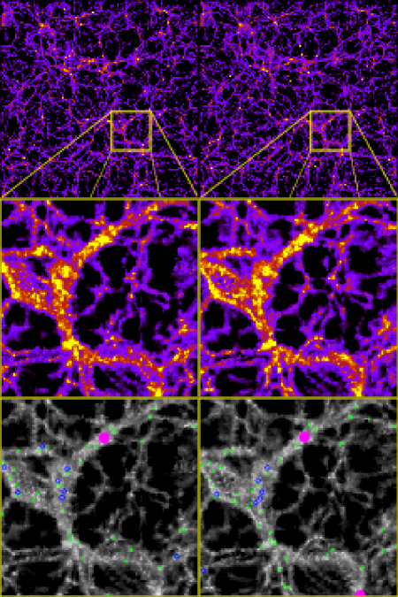
Figure 1.— Slices of thickness $0.2h^{-1}\mathrm{Mpc}$ from two cosmological models: $\Lambda$CDM (left), SUGRA (right). Top: $200h^{-1}\times 200h^{-1}\mathrm{Mpc}$ slices. Middle & Bottom: zoom-in, $40h^{-1}\times 40h^{-1}\mathrm{Mpc}$ slices. Middle: density field. Bottom: halo distribution, superimposed.

Here we introduce a new topological measure that is particularly suited to differentiating web-like structures. To this end, we advance the topological characterization of the Cosmic Web to a more complete description, the homology of the distribution as measured by the scale-dependent Betti numbers of the sample (Edelsbrunner & Muecke, 1994; Edelsbrunner & Harer, 2010; Robins, 2006; van de Weygaert et al., 2010, 2011). The Betti numbers underlie genus analysis and may be regarded as fundamental topological structure indicators that specifically characterise the homology of the distribution. While a full quantitative characterization of the topology of the cosmic mass distribution may not be feasible, the homology is an attractive compromise, providing a usefully detailed summary measurement of topology with relatively low computational overhead (e.g. Delfinado & Edelsbrunner, 1993; Edelsbrunner & Muecke, 1994).

1.1. Dark energy and the Cosmic Web

The parameters for what might now be called “the standard model for cosmology” have been established with remarkable precision. However, there remains the great mystery of the nature of the so-called “dark energy” (DE) which appears to make up some 73% of the total cosmic energy density. The simplest model for the dark energy is Einstein’s cosmological constant, $\Lambda$: this makes a constant, time independent, contribution to the total energy density in the Friedman-Lemaitre equations. Models based on this are referred to as “$\Lambda$CDM models”. However, there are numerous, possibly more plausible, models in which the dark energy evolves as a function of time. These models are generally described in terms of a time or redshift dependent function $w(z)$ that describes the history of equation of state of the dark energy component:

$$p=w(z)\rho c^{2}$$ (1)

Different models for dark energy produce different functions $w(z)$. The Einstein cosmological constant corresponds to $w(z)=-1$.

The aim of this paper is to compare, at redshift $z=0$, the topology of the cosmic structure in simulations of three cosmological models having different dark energy content that evolved from the same initial conditions (fig. 1). The equation of state of the dark energy models are those of the standard $\Lambda$CDM model and two quintessence models. The latter assume that the Universe contains an evolving quintessence scalar field, whose energy content manifests itself as dark energy. The two quintessence models are the Ratra-Peebles (RP) model and a SUGRA model (for a detailed description, see Ratra & Peebles, 1988; Amendola, 2000; Brax & Martin, 1999; Perrotta et al., 2000; de Boni et al., 2011; Bos et al., 2011).

2. Topology and Homology

2.1. Betti Numbers

Formally, homology groups and Betti numbers characterize the topology of a space in terms of the relationship between the cycles and boundaries we find in the space(Munkres, 1995; Zomorodian, 2005; Edelsbrunner & Harer, 2010).

For example, if the space is a $d$-dimensional manifold, ${{\mathbb{M}}}$, we have cycles and boundaries of dimension $p$ from $0$ to $d$. Correspondingly, ${{\mathbb{M}}}$ has one homology group $H_{p}({{\mathbb{M}}})$ for each of $d+1$ dimensions, $0\leq p\leq d$. By taking into account that two cycles should be considered identical if they differ by a boundary, one ends up with a group $H_{p}({{\mathbb{M}}})$ whose elements are the equivalence classes of $p$-cycles. The rank of the homology group $H_{p}({{\mathbb{M}}})$ is the $p$-th Betti number, ${{\beta}}_{p}={{\beta}}_{p}({{\mathbb{M}}})$.

In heuristic - and practical - terms, the Betti numbers count topological features and can be considered as the number of $p$-dimensional holes. When talking about a surface in $3$-dimensional space, the zeroth Betti number, ${{\beta}}_{0}$, counts the components or “islands”, the first Betti number, ${{\beta}}_{1}$, counts the tunnels, and the second Betti number, ${{\beta}}_{2}$, counts the enclosed voids. All other Betti numbers are zero.

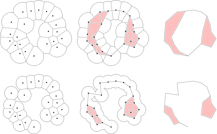
Figure 2.— Illustration of alpha shapes. For two different values of $\alpha$ (top: large $\alpha$; bottom: small $\alpha$), we show the relation between the $2$-dimensional point distribution, the value of $\alpha$, and the resulting alpha shape. Around each point in the sample, we draw a circle of radius $\alpha$. The outline of the corresponding Voronoi tessellation is indicated by the edges (left). All Delaunay simplices dual to the decomposition of the union of disks by the Voronoi polygons are shown in black (vertices and edges) and red (triangles) (center). The resulting alpha shape is shown on the right.

2.2. Genus and the Euler characteristic

Numerous cosmological studies have considered the genus of the isodensity surfaces defined by the megaparsec galaxy distribution (Gott et al., 1986; Hamilton et al., 1986; Choi et al., 2010), which specifies the number of handles defining the surface. The genus has a simple relation to the Euler characteristic, ${\chi}$, of the isodensity surface. Consider a $3$-manifold subset ${{\mathbb{M}}}$ of the Universe and its boundary, $\partial{{\mathbb{M}}}$, which is a $2$-manifold. With $\partial{{\mathbb{M}}}$ consisting of $c={{\beta}}_{0}(\partial{{\mathbb{M}}})$ components, the Gauss-Bonnet Theorem states that the genus of the surface is given by

$$G = c-\frac{1}{2}{\chi}(\partial{{\mathbb{M}}}),$$ (2)

where the Euler characteristic ${\chi}(\partial{{\mathbb{M}}})$ is the integrated Gaussian curvature of the surface

$${\mbox{$\chi$}}(\partial{{\mathbb{M}}}) = \frac{1}{2\pi}\oint_{x}\frac{{\rm\,d}x}{R_{1}(x)R_{2}(x)}.$$ (3)

Here $R_{1}(x)$ and $R_{2}(x)$ are the principal radii of curvature at point $x$ of the surface. The integral of the Gaussian curvature is invariant under continuous deformation of the surface: perhaps one of the most surprising results in differential geometry.

According to the Euler-Poincaré Formula, the Euler characteristic of the manifold ${{\mathbb{M}}}$ is equal to the alternating sum of its Betti numbers,

$${\chi}({{\mathbb{M}}})={{\beta}}_{0}({{\mathbb{M}}})-{{\beta}}_{1}({{\mathbb{M}}})+{{\beta}}_{2}({{\mathbb{M}}})\,.$$ (4)

For practical circumstances the third Betti number vanishes, ${{\beta}}_{3}({{\mathbb{M}}})=0$. The Euler characteristic of the boundary, $\partial{{\mathbb{M}}}$, is directly proportional to that of the Euler characteristic of the 3-manifold, ${{\mathbb{M}}}$, (Seifert & Threlfall, 1934, p.223)

$${\mbox{$\chi$}}(\partial{{\mathbb{M}}}) = 2{\chi}({{\mathbb{M}}}).$$ (5)

The combination of these equations for the Euler characteristic establishes a fundamental relationship between differential geometry and algebraic topology.

In the analysis described in this paper, we restrict ourselves to the three Betti numbers, ${{\beta}}_{0}$, ${{\beta}}_{1}$, and ${{\beta}}_{2}$, of the $3$-manifolds with boundary defined by the cosmic mass distribution. In an upcoming paper, we study genus and Betti number characteristics of Gaussian fields (Park et al., 2011).

3. Alpha Shapes

One of the key concepts in the field of Computational Topology is alpha shapes, introduced by Edelsbrunner and collaborators (Edelsbrunner et al., 1983; Muecke, 1993; Edelsbrunner & Muecke, 1994; Edelsbrunner, 2009). They generalize the convex hull of a point set and are concrete geometric objects that are uniquely defined for a particular point set $S$ and a scale $\alpha$. For their definition, we look at the union of balls of radius $\alpha$ centered on the points in the set, and its decomposition by the corresponding Voronoi tessellation. The alpha complex consists of all Delaunay simplices that record the subsets of Voronoi cells that have a non-empty common intersection within this union of balls (fig. 2).

The alpha complex thus consists of all simplices in the Delaunay triangulation that have an empty circumsphere with radius less than or equal to $\alpha$. Here “empty” means that the open ball bounded by the sphere does not include any points of $S$. For the extreme value $\alpha=0$, the alpha complex merely consists of the vertices of the point set. There is also a smallest value, $\alpha_{\max}$, such that for $\alpha\geq\alpha_{\max}$, the alpha complex is the Delaunay triangulation. The alpha shape is the union of simplices in the alpha complex and for $\alpha\geq\alpha_{\max}$ the alpha shape is the convex hull of the point set.

The alpha shape is a polytope in a fairly general sense: it can be concave and even disconnected. Its components can be three-dimensional clumps of tetrahedra, two-dimensional patches of triangles, one-dimensional strings of edges, and collections of isolated points, as well as combinations of these four types.

Alpha shapes reflect the topological structure of a point distribution on a scale parameterized by the real number $\alpha$. Figure 3 shows the $\alpha$-shape applied to a slice of a cosmological model. The three inserts show $\alpha$-shapes at three different $\alpha$ values.

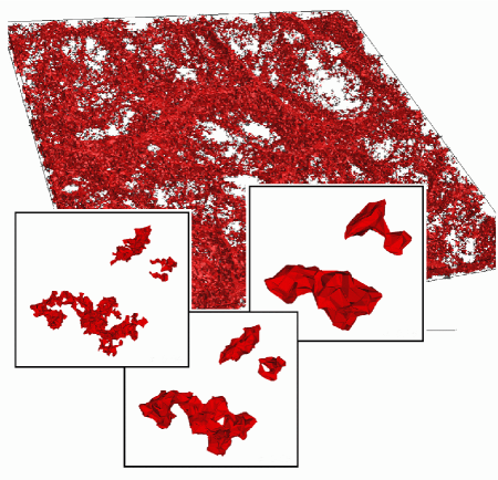
Figure 3.— Top: $\alpha$ shape of a GIF $\Lambda$CDM simulation, slice through simulation box. Bottom: $\alpha$ shape at 3 different values of $\alpha$.

3.1. Filtrations

The concept of “filtration” is an important source of information about the topology of a point distribution. A filtration provides a view of the topology as a function of scale. Formally, given a space ${{\mathbb{M}}}$, a filtration is a nested sequence of subspaces:

$$\emptyset={{\mathbb{M}}}_{0}\subseteq{{\mathbb{M}}}_{1}\subseteq\ldots\subseteq{{\mathbb{M}}}_{m}={{\mathbb{M}}}.$$ (6)

The nature of the filtrations depends, amongst other things, on the representation of the mass distribution. For a discrete point distribution, the set of alpha shapes, ordered by scale, constitute a filtration of the Delaunay tessellation.

The set of real numbers $\alpha$ leads to a family of shapes capturing the intuitive notion of the overall versus fine shape of a point set. Starting from the convex hull gradually decreasing $\alpha$, the shape of the point set gradually shrinks and starts to develop enclosed voids. These voids may join to form tunnels and larger voids. For negative $\alpha$, the alpha shape is empty.

Although the alpha shape is defined for all real numbers $\alpha$, there are only a finite number of different alpha shapes for any finite point set. In other words, the alpha shape process proceeds discretely with increasing $\alpha$, marked by the addition of new Delaunay simplices once $\alpha$ exceeds the corresponding threshold.

3.2. Computing Betti Numbers

The standard algorithm in 2-D and 3-D for calculating Betti numbers of an $\alpha$-complex is due to Delfinado & Edelsbrunner (1993). The algorithm is efficient in the sense that only one traversal of the simplices making up the $\alpha$ complex is required. First, the Delaunay tessellation of the point set is constructed. Its simplices - vertices, edges, triangles - can be ordered by the radius of the smallest sphere that touches the points defining the given simplex and contains no other data points. From this ordering a nested sequence of subcomplexes can be constructed, each member of the sequence being constructed from the preceding one by the addition of a new simplex having a larger scale. If for example the added simplex is an edge, it will either connect two previously disjoint components or close a loop (thereby creating a tunnel).

Cycling through all its simplices, in three dimensions the calculation is based on the following straightforward considerations. When a vertex is added to the alpha complex, a new component is created and ${{\beta}}_{0}$ is increased by $1$. Similarly, if an edge is added, it connects two vertices, which either belong to the same or to different components of the current complex. In the former case, the edge creates a new tunnel, so ${{\beta}}_{1}$ is increased by $1$. In the latter case, two components get connected into one, so ${{\beta}}_{0}$ is decreased by $1$. If a triangle is added, it either completes a void or it closes a tunnel. In the former case, ${{\beta}}_{2}$ is increased by $1$, and in the latter case, ${{\beta}}_{1}$ is decreased by $1$. Finally, when a tetrahedron is added, a void is filled, so ${{\beta}}_{2}$ is lowered by $1$. Following this procedure, the algorithm has to include a technique for determining whether a $p$-simplex belongs to a $p$-cycle. For vertices and tetrahedra, this is rather trivial. For edges and triangles, a more elaborate procedure is necessary (Delfinado & Edelsbrunner, 1993).

For software that implements these algorithmic ideas, we resort to the Computational Geometry Algorithms Library, CGAL  (Caroli & Teillaud, 2011; Da & Yvinec, 2011).

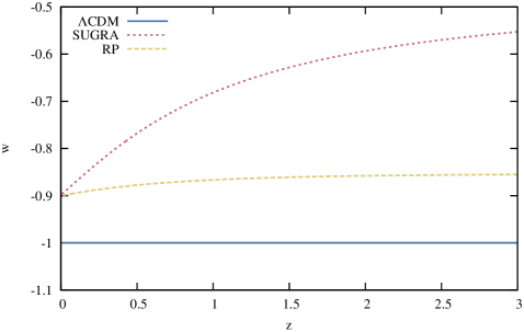
Figure 4.— Evolution of the dark energy equation of state parameter $w(z)$ for $\Lambda$CDM (solid), SUGRA (dotted) and RP (dashed).

4. Topological Analysis of simulations

4.1. Our simulations

We investigate the evolved structure in the standard $\Lambda$CDM model, the Ratra-Peebles (RP) model, and a SUGRA model. All simulations start with the primordial perturbation amplitudes and phases. The imprint of dark energy on the mass distribution is expressed via the different expansion history of the universe as a result of the differently evolving equation of state parameter $w(z)$ (fig. 4). This is determined by the evolution of the quintessence scalar field $\phi$, forced by a parameterized potential $V(\phi)$. The DE model parameters (table 1 in Bos et al. (2011)) are chosen such that the models differ significantly from $\Lambda$CDM, while still in accordance with observations. For example, the slope of the quintessence potentials is set to $\zeta_{\mathrm{RP}}=0.347$ and $\zeta_{\mathrm{SUGRA}}=2.259$.

The models we consider are described by WMAP7 (Larson et al., 2011) best-fit value parameters ($h=0.704$, $\Omega_{m}=0.272$, $\Omega_{\Lambda}=0.728$, $\sigma_{8}=0.809$ and $n_{s}=0.963$). For each model we ran $512^{3}$ and $256^{3}$ particle simulations, in a periodic box of $200h^{-1}\mathrm{Mpc}$ width, starting at $z\approx 63$. The baryonic content of the universe is incorporated as dark matter particles, using $\Omega_{m}=\Omega_{dm}+\Omega_{b}=0.272$.

We use the SUBFIND algorithm (Springel et al., 2001) to identify the gravitationally bound haloes in the resulting particle distributions. At $z=0$ the simulation boxes contain 170740 ($\Lambda$CDM), 172949 (RP) and 175332 (SUGRA) halos with mass higher than $M\sim 1.4\times 10^{11}h^{-1}{\rm M}_{\odot}$ ($>32$ particles). They trace the general structures present in the field, even though a lot of the detailed structure is lost or diluted (fig. 1).

Slices from two simulations, at $z=0$, are shown in figure 1. The left hand panel displays the standard $\Lambda$CDM model and the right hand panel shows the SUGRA model. The slices as shown in the upper panels are perceptually indistinguishable. Differences can only be perceived at higher resolution and lower contrast: this is shown in the lower panels of figure 1, for the dark matter density field as well as the haloes. Different filaments appear, the subclustering is different in the big cluster and there are a number of different voids. The voids differ in size and shape, and their degree of merging (cf. Sheth & van de Weygaert, 2004).

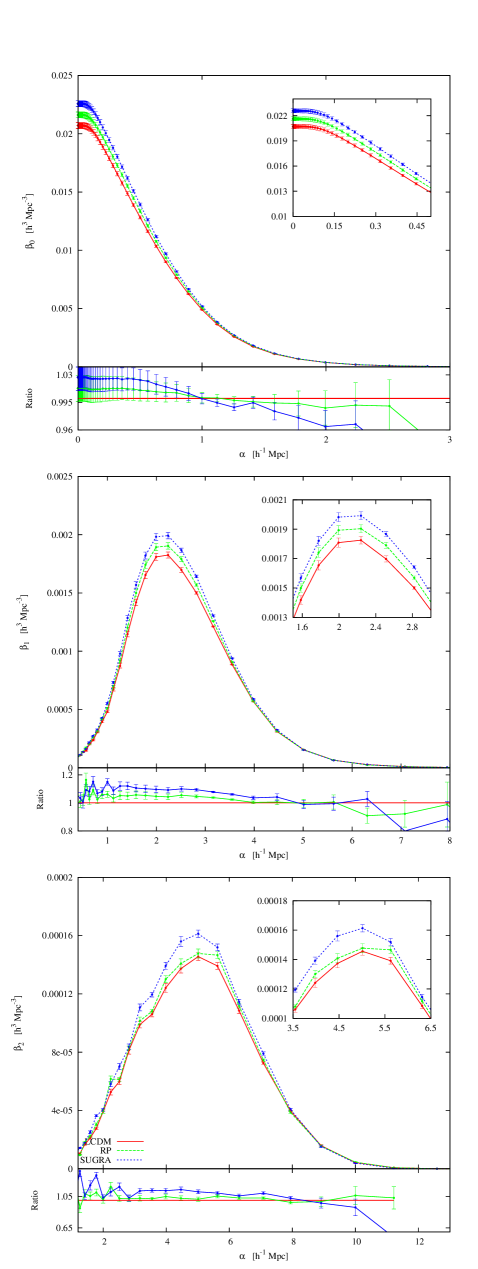
Figure 5.— Betti signatures: Betti numbers, per unit volume, as a function of scale $\alpha$ at $z=0$. Red: $\Lambda$CDM, Green: RP, Blue: SUGRA. Top: $\beta_{0}$; Middle: $\beta_{1}$; Bottom: $\beta_{2}$. Inserts: detailed differences near distribution peak. Lower strip: $\beta_{i}/\beta_{i}(\Lambda$CDM).

4.2. The analysis - Betti signatures

We analyse the clustering of the haloes in these three simulations using Betti Numbers. In order to compute the Betti numbers for a point distribution in 3 dimensions, we generate the Delaunay tessellation from the point sample and from this the nested sequence of alpha shapes. Subsequently, we determine the Betti numbers of the set of alpha shapes as a function of $\alpha$. The resulting Betti number versus $\alpha$ curves are the Betti signature of the point distribution. In Figure 4 we show the Betti signatures for the scale dependence of $\beta_{0}(\alpha)$, $\beta_{1}(\alpha)$, and $\beta_{2}(\alpha)$ in the three simulations. The error bars in all panels are derived on the basis of estimates from 8 sub-cubes. There are significant differences between the curves for $\beta_{1}(\alpha)$, and $\beta_{2}(\alpha)$ in the three models, showing that the Betti signature is a sensitive discriminator of structure, even in a single redshift slice. This remains true when taking into account differences in $\beta_{0}$ and $\sigma_{8}$. In subsequent papers we follow the evolution of the Betti signature with time and assess their dependence on halo mass and show that it provides a sensitive measure of the nature of dark energy.

5. Discussion and Conclusions

We have presented a powerful topology-based method for classifying the structure that develops in cosmological N-body simulations. The Betti signatures are an effective way of discriminating between models that superficially look the same. The method is an important generalisation of the genus and Minkowski functional approaches, in that Betti analysis of alpha shapes is able to discriminate structural content at a deeper level (Robins, 2006; van de Weygaert et al., 2010, 2011).

The Betti signatures of the cosmological simulations are shown to be capable of discriminating between models that are difficult to distinguish by other means. This may involve dark energy signatures or traces of primordial non-Gaussianities in the cosmic mass distribution. This is because dark energy affects the expansion of the universe, which affects the formation of nonlinear objects, while non-Gaussian initial conditions will change the formation history of galaxies and thus Betti numbers.

It is also important to put our approach in terms of Betti analysis in perspective relative to other measures of structure, in particular the Minkowski functionals (Mecke et al., 1994; Schmalzing & Buchert, 1997). While the Euler characteristic and Betti numbers give information about the connectivity of a manifold, the other three Minkowski functionals are sensitive to local manifold deformations. The Minkowski functionals give information about the metric properties of a manifold on the basis of which broad-brush structural characteristics such as shape can be defined (Sahni et al., 1998). The Betti numbers focus on its topological properties, the scale dependence likewise providing some metric information.

In a series of following papers we shall be adding the powerful notion of topological persistence (Edelsbrunner et al., 2002) to our analysis of filtrations (Pranav et al., 2011). Betti analysis is an integral part of an intrinsically much richer topological language which addresses the hierarchical substructure of the Cosmic Web in an elegant and natural description (for a cosmological application, see Sousbie, 2011; Sousbie et al., 2011). In standard practice, the multiscale nature of the mass distribution tends to be investigated by means of user-imposed filtering. Persistence entails the conceptual framework and language for separating scales of a spatial structure, and rationalizes the multiscale approach by considering the range of filters at once. At the same time, it deepens the approach by combining it with topological measurements. Within the context of hierarchical cosmic structure formation, persistence therefore provides a natural formalism for a multiscale topology study of the Cosmic Web. Alpha shapes provide the perfect context for understanding the concept: the position of a feature within the structural hierarchy is determined by the $\alpha$ interval over which it persists. Persistence even provides a natural path towards removing topological noise, which would be identified as features with small persistence (see van de Weygaert et al., 2011).

References

- Amendola (2000) Amendola, L., 2000, PhRvD, 62, 3511
- Bond et al. (1996) Bond, J.R., Kofman, L., & Pogosyan, D., 1996, Nature, 380, 603
- Bos et al. (2011) Bos, E.G.P., van de Weygaert, R., Dolag, K., & Pettorino, V., 2011, MNRAS, to be subm.
- Brax & Martin (1999) Brax, P.H., & Martin, J., 1999, Phys.Lett. B, 468, 40
- Choi et al. (2010) Choi, Y.-Y., Park, C., Kim, J., Gott, J.R., Weinberg, D.H., Vogeley, M.S., & Kim, S.S., 2010, ApJS, 190, 181
- Colless et al. (2003) Colless, M., et al., 2003, astro-ph/0306581
- de Boni et al. (2011) de Boni, C., Dolag, K., Ettori, S., Moscardini, L., Pettorino, V., & Baccigalupi, C., 2011, MNRAS, 414, 780
- Caroli & Teillaud (2011) Caroli, M., & Teillaud, M., 2011, 3D Periodic Triangulations, CGAL User and Reference Manual, CGAL Editorial Board, 3.9 edition, ch. 40.
- Da & Yvinec (2011) Da, T.K.F., & Yvinec, M., 2011, 3D Alpha Shapes, CGAL User and Reference Manual, CGAL Editorial Board, 3.9 edition, ch. 42.
- Delfinado & Edelsbrunner (1993) Delfinado, C.J.A., & Edelsbrunner, H., 1993, in Symposium on Comput. Geometry, DBLP, 232
- Edelsbrunner et al. (1983) Edelsbrunner, H., Kirkpatrick, D., & Seidel, R., 1983, IEEE Trans. Inform. Theory, 29, 551
- Edelsbrunner & Muecke (1994) Edelsbrunner, H., & Muecke, E.P., 1994, ACM Trans. Graphics, 13, 43
- Edelsbrunner et al. (2002) Edelsbrunner, H., Letscher, D., & Zomorodian, A., 2002, Discrete and Comput. Geometry, 28, 511
- Edelsbrunner (2009) Edelsbrunner, H., 2011, in Tessellations in the Sciences: Virtues, Techniques and Applications of Geometric Tilings, eds. R. van de Weygaert, G. Vegter, J. Ritzerveld & V. Icke, 2011, Springer Verlag
- Edelsbrunner & Harer (2010) Edelsbrunner, H., & Harer, J., 2010, Computational Topology, An Introduction, AMC, 241 pp.
- Gott et al. (1986) Gott, J.R., Dickinson, M., & Melott, A.L., 1986, ApJ, 306, 341
- Gott et al. (2005) Gott, J.R., Juríc, M., Schlegel, D., Hoyle, F., Vogeley, M., Tegmark, M., Bahcall, N., & Brinkmann, J., 2005, ApJ, 624, 463
- Hamilton et al. (1986) Hamilton, A. .J. S., Gott, J.R., & Weinberg, D., 1986, ApJ, 309, 1
- Huchra et al. (2005) Huchra, J., et al., 2005, in Nearby Large-Scale Structures and the Zone of Avoidance, eds. A.P. Fairall, P.A. Woudt, ASP Conf. Ser. Vol., 239, 135
- Larson et al. (2011) Larson, D., Dunkley J., Hinshaw, G., Komatsu, E., Nolta, M.R., Bennett, C.L., Gold, B., Hapern, M., Hill, R.S., Jarosik, N., Kogut, A., Limon, M., Meyer, S.S., Odegard, N., Page, L., Smith, K.M., Spergel, D.N., Tucker, G.S., Weiland, J.L., Wollack, E., & Wright, E.L., 2011, ApJS, 192, 16
- Mecke et al. (1994) Mecke, K.R., Buchert, T., & Wagner, H., 1994, A&A, 288, 697
- Muecke (1993) Muecke, E.P., 1993, Shapes and Implementations in three-dimensional geometry, PhD thesis, Univ. Illinois Urbana-Champaign
- Munkres (1995) Munkres, J.R., 1995, Elements of Algebraic Topology, Westview Press
- Park et al. (2011) Park, C., Pranav, P., Chingangbam, P., van de Weygaert, R., Vegter, G., Kim, I.K., Edelsbrunner, H., Hellwing, W.A., & Hidding, J., 2011, ApJ, to be subm.
- Perrotta et al. (2000) Perrotta, F., Baccigalupi, C., & Matarrese, S., 2000, PhRvD, 61, 3507
- Pranav et al. (2011) Pranav, P., Edelsbrunner, H., van de Weygaert, R., & Vegter, G., 2011, MNRAS, to be subm.
- Ratra & Peebles (1988) Ratra, B., & Peebles, P.J.E., 1988, Phys. Rev. D., 37, 3406
- Robins (2006) Robins, V., 2006, Phys. Rev. E., 74, 061107
- Sahni et al. (1998) Sahni, V., Sathyaprakash, B.S., & Shandarin, S.F., 1998, ApJ, 495, 5
- Schmalzing & Buchert (1997) Schmalzing, J., Buchert, T., 1997, ApJ, 482, 1
- Seifert & Threlfall (1934) Seifert, H., Threlfall, W., 1934, Lehrbuch der Topologie, Leipzig: Teubner
- Sheth & van de Weygaert (2004) Sheth, R., & van de Weygaert, R., 2004, MNRAS, 350, 517
- Sousbie (2011) Sousbie, T., 2011, MNRAS, 414, 1
- Sousbie et al. (2011) Sousbie, T., Pichon, C., & Kawahara, H., 2011, MNRAS, 414, 384
- Springel et al. (2001) Springel, V., White, S.D.M., Tormen, G., & Kauffmann, G., 2001, MNRAS, 328, 726
- van de Weygaert & Bond (2008) van de Weygaert, R., & Bond, J.R. 2008, Clusters and the Theory of the Cosmic Web. In: A Pan-Chromatic View of Clusters of Galaxies and the Large-Scale Structure, eds. M. Plionis, O. Lopez-Cruz, D. Hughes, Lect. Notes Phys., 740, 335 (Springer)
- van de Weygaert et al. (2010) van de Weygaert, R., Platen, E., Vegter, G., Eldering, B., & Kruithof, N., 2010, in 2010 Int’l Symposium on Voronoi in Science and Engineering, IEEE, p. 224
- van de Weygaert et al. (2011) van de Weygaert, R., Vegter, G., Edelsbrunner, H., Jones, B.J.T., Pranav, P., Park, C., Hellwing, W.A., Eldering, B., Kruithof, N., Bos, E.G.P., Hidding, J., Feldbrugge, J., ten Have, E., van Engelen, M., Caroli, M., & Teillaud, M., 2011, Trans. on Comput. Sci. XIV, LNCS 6970, pp. 60-101
- Zomorodian (2005) Zomorodian, A.J., 2005, Topology for Computing, Cambr. Univ. Press