Geometric phase in the Kitaev honeycomb model and scaling behavior at critical points

Abstract

In this paper a geometric phase of the Kitaev honeycomb model is derived and proposed to characterize the topological quantum phase transition. The simultaneous rotation of two spins is crucial to generate the geometric phase for the multi-spin in a unit-cell unlike the one-spin case. It is found that the ground-state geometric phase, which is non-analytic at the critical points, possesses zigzagging behavior in the gapless $B$ phase of non-Abelian anyon excitations, but is a smooth function in the gapped $A$ phase. Furthermore, the finite-size scaling behavior of the non-analytic geometric phase along with its first- and second-order partial derivatives in the vicinity of critical points is shown to exhibit the universality. The divergent second-order derivative of geometric phase in the thermodynamic limit indicates the typical second-order phase transition and thus the topological quantum phase transition can be well described in terms of the geometric-phase.

year number number identifier

I Introduction

Berry in his pioneer work raised a fundamentally important concept known as geometric phase (GP) in addition to the usual dynamic phase accumulated on the wave function of a quantum system, provided that the Hamiltonian varies with multi-parameters cyclically and adiabatically Berry . At the present time the GP with extensive generalization along many directions has wide applications in various branches of physics Berry2 ; Shapere ; Bohm .

Recently, the close relation between GP and quantum phase transition (QPT) has been gradually revealed Carollo ; Zhu ; Hamma and increasing interest has been drawn to the role of GP in detecting QPT for various many-body systems Zhu08 ; Chen ; interests , which, as a matter of fact, is also a new research field in condensed matter physics Sachdev ; Sondhi . QPT usually describes an abrupt change in the ground state of a many-body system induced by quantum fluctuations. The phase transition between ordered and disordered phases is accompanied by symmetry breaking, which can also be characterized by Landau-type order parameters.

On the other hand, a new type of QPT called topological quantum phase transitions (TQPT) has attracted much attention. The first non-trivial example is the fractional quantum Hall effect Tsui ; Laughlin . In the last decade, several exactly soluble spin-models with the TQPT, such as the toric-code model Kitaev03 , the Wen-plaquette model Wen-plaquette ; Wen08 and the Kitaev model on a honeycomb lattice Kitaev , were found. In contrast to the conventional QPT governed by local order parameters Sachdev , the TQPT can be characterized only by the topological order WenBook . As good examples to illustrate the underlying physics, different methods are developed to describe the TQPT in the Kitaev honeycomb model T. Xiang07 ; T. Xiang08 ; H. D. Chen07 ; H. D. Chen08 ; S. Yang ; Gu . In Ref. T. Xiang07 , Feng et.al. obtained the local order parameters of Landau type to characterize the phase transition by introducing Jordan-Wigner and spin-duality transformations into the Majorana representation of the honeycomb model. Gu et.al. showed an exciting result of the ground-state fidelity susceptibility S. Yang ; Gu , which can be used to identify the TQPT from the gapped $A$ phase with Abelian anyon excitations to gapless $B$ phase with non-Abelian anyon excitations.

Quite recently, Zhu Zhu showed that the ground-state GP in the $XY$ model is non-analytic with a diverged derivative with respect to the field strength at the critical value of magnetic field. Thereupon, the relation between the GP and the QPT is established. Nevertheless, much attention has been paid to the QPT, while effort devoted to the relation between the GP and the TQPT is very little. The present paper is devoted to exploiting the GP of the Kitaev honeycomb model as an essential tool to establish a relation between the GP and the TQPT and reveal the novel quantum criticality. Unlike the GP in the usual lattice-spin model for the QPT, which is generated by the single-spin rotation of each lattice-site, the simultaneous rotation of linked two spins in one unit-cell seems crucial to describe the TQPT in the honeycomb model. The non-analyticity of GP at the critical points with a divergent second-order derivative with respect to the coupling parameters shows that the TQPT is the second-order transition and can be well described by the GP.

In Sec. II, the ground state wave function and energy spectrum of the Kitaev honeycomb model are presented. After introducing a correlated rotation of two $z$-link spins in each unit-cell, the ground-state GP and its derivatives are obtained explicitly in Sec. III. Sec. IV is devoted to investigating the scaling behavior of the GP. A brief summary and discussion are given in Sec. V.

II The Kitaev honeycomb model and spectrum

The Kitaev honeycomb model shown in Fig. 1(a) is firstly introduced to illustrate the topologically fault-tolerant quantum-information processing Kitaev03 ; Kitaev ; Nayak . In this model, each spin located at vertices of the lattice interacts with three nearest-neighbor spins through three types of bonds, depending on their directions. By using the Pauli operators $\sigma^{a}$ $(a=x,y,z)$, the corresponding Hamiltonian is written as

$$H=-J_{x}\!\!\!\sum_{x\mbox{-links}}\!\!\!\sigma_{j}^{x}\sigma_{k}^{x}-J_{y}\!\!\!\sum_{y\mbox{-links}}\!\!\!\sigma_{j}^{y}\sigma_{k}^{y}-J_{z}\!\!\!\sum_{z\mbox{-links}}\!\!\!\sigma_{j}^{z}\sigma_{k}^{z},$$ (1)

where $j$, $k$ denote the two ends of the corresponding bond, and $J_{a}$ are coupling parameters. After introducing a special notation $K_{jk}=\sigma_{j}^{a}\sigma_{k}^{a}$, where the indexes $a$ depend on the types of links between sites $j$ and $k$ (so we also write it into $a_{jk}$ in the following text for perspicuousness), Hamiltonian (1) can be rewritten into a compact form

$$H=-\frac{1}{2}\sum_{\langle j,k\rangle}J_{a_{jk}}K_{jk}.$$ (2)

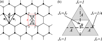
Figure 1: (Color online) (a) Kitaev honeycomb model, in which one spin interacts with three nearest-neighbor spins through three types of bonds, depending on their direction. A unit-cell with $x$, $y$ and $z$ links and graphic representation of Hamiltonian (4) with Majorana operators are marked by the red dotted line. (b) Phase diagram of the model, where $A$ phase is gapped and $B$ phase is gapless.

It has been known that the Kitaev honeycomb model can be solved exactly by introducing Majorana fermion operators, which are defined as Kitaev ; S. Yang

$$\sigma^{x}=ib^{x}c,\quad\sigma^{y}=ib^{y}c,\quad\sigma^{z}=ib^{z}c.$$ (3)

Generally, a set of Majorana operators $M=\left\{b^{x},b^{y},b^{z},c\right\}$ can be employed to describe a spin by two fermionic modes. They are Hermitian and obey the relations $m^{2}=1$ and $mm^{\prime}=-m^{\prime}m$ for $m,m^{\prime}\in M$ and $m\neq m^{\prime}$. Moreover, in the Hilbert space with a spin described by two fermionic modes, the relation $b^{x}b^{y}b^{z}c\left|\Psi\right\rangle=\left|\Psi\right\rangle$ must be satisfied to ensure the obeying of the same algebraic relations as $\sigma^{x}$, $\sigma^{y}$, and $\sigma^{z}$ Kitaev .

Drawing on the operators (3) to the Kitaev honeycomb model, Hamiltonian (2) is given by

$$H=\frac{i}{2}\sum_{\langle j,k\rangle}\hat{u}_{jk}J_{a_{jk}}c_{j}c_{k},$$ (4)

where $\hat{u}_{jk}=ib_{j}^{a_{jk}}b_{k}^{a_{jk}}$. Fig. 1(a) also shows the structure of Hamiltonian (4), from which it can be seen that $\hat{u}_{jk}=-\hat{u}_{kj}$. Since these operators $\hat{u}_{jk}$ commute with the Hamiltonian (4) and with each other, the Hilbert space splits into two common eigenspaces of $\hat{u}_{jk}$ with eigenvalues $u_{jk}=\pm 1$. Thus, Hamiltonian (4) is reduced to a quadratic Majorana fermionic Hamiltonian

$$H=\frac{i}{2}\sum_{\langle j,k\rangle}u_{jk}J_{a_{jk}}c_{j}c_{k}.$$ (5)

With a Fourier transformation

$$c_{s,\lambda}=\frac{1}{\sqrt{2L^{2}}}\sum_{\mathbf{q}}e^{i\mathbf{q}\cdot\mathbf{r}_{s}}a_{\mathbf{q},\lambda},$$ (6)

where $s$ denotes a unit cell shown in Fig. 1(a), $\lambda$ refers to a position inside the cell, $r_{s}$ represents the coordinate of the unit cell, and $\mathbf{q}$ are momenta of the system with finite system-size $2L^{2}$, and a Bogoliubov transformation

$$\left\{\begin{array}[]{c}C_{\mathbf{q},1}^{{\dagger}}=\frac{1}{\sqrt{2}}a_{-\mathbf{q},1}-\frac{1}{\sqrt{2}}A_{\mathbf{q}}^{\ast}a_{-\mathbf{q},2},\\ C_{\mathbf{q},2}^{{\dagger}}=\frac{1}{\sqrt{2}}A_{\mathbf{q}}a_{-\mathbf{q},1}+\frac{1}{\sqrt{2}}a_{-\mathbf{q},2},\end{array}\right.$$ (7)

where $A_{\mathbf{q}}=\sqrt{\epsilon_{\mathbf{q}}^{2}+\Delta_{\mathbf{q}}^{2}}/(\Delta_{\mathbf{q}}+i\epsilon_{\mathbf{q}})$, Hamiltonian (5) is transformed into

$$H=\sum_{\mathbf{q}}\sqrt{\epsilon_{\mathbf{q}}^{2}+\Delta_{\mathbf{q}}^{2}}\left(C_{\mathbf{q},1}^{\dagger}C_{\mathbf{q},1}-C_{\mathbf{q},2}^{\dagger}C_{\mathbf{q},2}\right)$$ (8)

with $\epsilon_{\mathbf{q}}=J_{x}\cos q_{x}+J_{y}\cos q_{y}+J_{z}$, and $\Delta_{\mathbf{q}}=J_{x}\sin q_{x}+J_{y}\sin q_{y}$. In Hamiltonian (8), the momenta take the values S. Yang

$$q_{x\left(y\right)}=\frac{2n\pi}{L},n=-\frac{L-1}{2},\cdots,\frac{L-1}{2},$$ (9)

when the system size is chosen as $N=2L^{2}$ with $L$ being an odd integer. Thus, the ground and the first-excited states are obtained by

$$\left|\Psi_{0}\right\rangle \!\!=\prod_{\mathbf{q}}C_{q,2}^{\dagger}\left|0\right\rangle=\prod_{\mathbf{q}}\frac{1}{\sqrt{2}}\left(A_{\mathbf{q}}a_{-\mathbf{q},1}+a_{-\mathbf{q},2}\right)\left|0\right\rangle,$$ (10)

$$\left|\Psi_{1}\right\rangle \!\!=\prod_{\mathbf{q}}C_{q,1}^{\dagger}\left|0\right\rangle=\prod_{\mathbf{q}}\frac{1}{\sqrt{2}}\left(a_{-\mathbf{q},1}-A_{\mathbf{q}}^{\ast}a_{-\mathbf{q},2}\right)\!\left|0\right\rangle,$$ (11)

with the energy eigenvalues

$$E_{0,1}=\pm\sum_{\mathbf{q}}\sqrt{\epsilon_{\mathbf{q}}^{2}+\Delta_{\mathbf{q}}^{2}},$$ (12)

It has been shown that the Kitaev honeycomb model (1) has a rich phase diagram including a gapped phase with Abelian anyonic excitations (called $A$ phase) and a gapless phase with non-Abelian anyonic excitations ($B$ phase) Kitaev . In Fig. 1(b), the two phases $A$ and $B$ are separated by three transition lines, i.e., $J_{x}=1/2$, $J_{y}=1/2$, and $J_{z}=1/2$, which form a small triangle surrounding the $B$ phase. Here, we only plot the energy spectrum (12) as a function of $J_{z}$ for $J_{x}=J_{y}$ (the vertical dot-and-dash line in Fig. 1(b)) in Fig. 2. It can be seen from Fig. 2 that the energy-level degeneracy arises or lifts at certain points, which can be regarded as the possible critical points of QPT Zhu ; Sachdev . In Fig. 2(b, c, d), the degenerate points occur in the $B$ phase, but disappear in the $A$ phase as shown in Fig. 2(f). Moreover, the energy spectrum may have asymptotic degeneracy at the phase diagram edge seen from Fig. 2(a) when the size of system tends to infinity. The non-analyticity points of ground state in $B$ phase are actual level-crossing points.

.

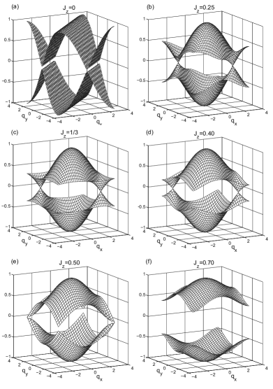
Figure 2: Energy spectrum for the parameters $J_{x}=J_{y}$ (a) $J_{z}=0$, the spectrum indeed is degenerate in a larger system size; (b), (c), and (d) in $B$ phase, for $J_{z}<1/3$, $J_{z}=1/3$, and $1/3<J_{z}<1/2$, respectively; (e) at the critical point of $J_{z}=1/2$ and (f) in $A$ phase. It is clearly that there is level-crossing in (b), (c) and (d).

III Geometric phase

In general spin-chain systems characterized by Landau-type order parameters, the GPs can be generated by adiabatic and cyclic evolutions with a rotation of each spin coupled with its neighbors in the certain parameter spaces Zhu . However, in the Kitaev honeycomb model, the two spins $\sigma_{s,\lambda}$ and $\sigma_{s,\bar{\lambda}}$ in the unit cell $s$ is coupled with each other only by a $z$-link, as Fig. 1(a) shows. As a result, a simple rotation of a single-spin with the generator $\sigma_{s,\lambda}^{z}$ can only ”propagate” along the horizontal spin-chain through the $x$- and $y$-link couplings but not along the vertical direction since the rotation-generator of a single-spin $\sigma_{s,\lambda}^{z}$ commutes with the $z$-link spin-operators in the Hamiltonian between the horizontal spin-chains. On other words, if using the above single-spin rotation, the Kitaev honeycomb model would be equivalent to a system of independent multi-single-spin-chains. In order to obtain the GP of the Kitaev honeycomb model, it should be introduced a correlated rotation of two $z$-link spins in each unit-cell,

$$U\left(\phi\right)=\exp\left[i\phi R\right],$$ (13)

where

$$R=\sum_{s}\sum_{\lambda}\sigma_{s,\lambda}^{z}\sigma_{s,\bar{\lambda}}^{z}$$ (14)

is the correlated rotation-generator, and $\phi$ is the ”co-rotation angle”. Indeed, when the rotation operator is applied on the spin of $\left(s,\lambda\right)$-th set, the spin operator $\sigma_{s,\bar{\lambda}}^{z}$ acts as a c-number because the spin operators on different sets commute each other. As a matter of fact, the correlated rotation-generator $R$ can generate a ”co-rotation” of the $z$-link spins in each unit cell. Furthermore, under the gauge transformation (13), the rotations of each spins in the 2D honeycomb Kitaev model become correlative and global. Hence it is possible to reveal the relation between the GP and the nonlocal TQPT by means of the correlated rotation. Then, the ground state wave function becomes

$$\left|\Psi_{0}^{\prime}(\phi)\right\rangle=U\left(\phi\right)\left|\Psi_{0}\right\rangle,$$ (15)

and correspondingly, the GP is given by Liang

$$\gamma =-i{\int\nolimits_{0}^{2\pi}}\left\langle\Psi_{0}\right|U^{{}^{{\dagger}}}\frac{d}{d\phi}U\left|\Psi_{0}\right\rangle d\phi$$

$$=-2\pi\left\langle\Psi_{0}\right|R\left|\Psi_{0}\right\rangle.$$ (16)

It can be seen that the GP for the Kitaev honeycomb model is proportional to the expectation value of the correlated rotation $R$. Different from the local spin-correlation $\sigma_{s,\lambda}^{z}\sigma_{s,\bar{\lambda}}^{z}$, the sum over whole lattice-sites in $R$ leads to a global property, which is crucial for the topological QPT.

In terms of the Majorana fermion operators (3), the rotation operator $R$ is given, after using the Fourier transformation (6), by $R=\sum_{s,\lambda}\left(ib_{s,\lambda}^{z}c_{s,\lambda}\right)\left(ib_{s,\bar{\lambda}}^{z}c_{s,\bar{\lambda}}\right)=\sum_{s}\left(-iu_{s,1;s,2}^{z}c_{s,1}c_{s,2}\right)+\sum_{s}\left(-iu_{s,2;s,1}^{z}c_{s,2}c_{s,1}\right)$. Under the restriction of vortex free subspace, $u_{s,1;s,2}^{z}$ and $u_{s,2;s,1}^{z}$ are the good quantum numbers, that is to say, $u_{s,1;s,2}^{z}=1$, and $u_{s,2;s,1}^{z}=-1$. Thus, the rotation operator $R$ is finally obtained by

$$R=\frac{-i}{\sqrt{2L^{2}}}\sum_{\mathbf{q}}\left(a_{-\mathbf{q},1}a_{\mathbf{q},2}-a_{-\mathbf{q},2}a_{\mathbf{q},1}\right).$$ (17)

By means of Eqs. (10), (16), and (17), the ground-state GP is given formally by

$$\gamma=\frac{-2\pi}{\sqrt{2L^{2}}}\sum_{\mathbf{q}}\mathop{\rm Im}\left(-A_{\mathbf{q}}e^{2i\mathbf{q}\cdot\mathbf{d}}+A_{\mathbf{q}}^{\ast}\right),$$ (18)

where $\mathbf{d}$ is a vector from one site to another inside one cell. It can be seen easily from Fig. 1(a) that the vector is given by $\mathbf{d=}\left(\mathbf{n}_{1}+\mathbf{n}_{2}\right)/3$. Inserting this vector $\mathbf{d}$ into Eq. (18), we have

$$\gamma \!\!=\!\!\frac{-2\pi}{\sqrt{2L^{2}}}\sum_{\mathbf{q}}\mathop{\rm Im}\left(-A_{\mathbf{q}}e^{\frac{i}{3}\left(2q_{x}+2q_{y}\right)}+A_{\mathbf{q}}^{\ast}\right)$$

$$\!\!=\!\!\frac{-2\pi}{\sqrt{2\!L^{2}}}\!\!\sum_{\mathbf{q}}\!\frac{\epsilon_{\mathbf{q}}\!\!\left[1\!\!+\!\cos\!\frac{1}{3}\!\left(2q_{x}\!\!+\!2q_{y}\!\right)\right]\!\!-\!\!\Delta_{\mathbf{q}}\sin\!\frac{1}{3}\!\left(2q_{x}\!\!+\!2q_{y}\right)}{\sqrt{\epsilon_{\mathbf{q}}^{2}+\Delta_{\mathbf{q}}^{2}}}$$ (19)

.

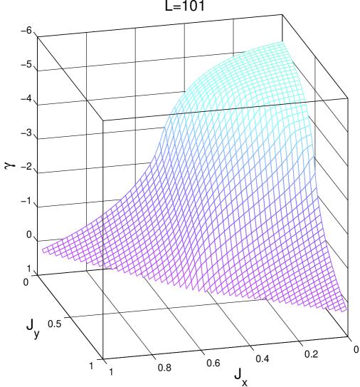
Figure 3: (Color online) Scaled GP with system size parameter $L=101$.

Eq. (19) is the main result of this paper. The scaled (or average) GP $\gamma/L$ as a function of coupling parameters is shown in Fig. 3, which distributes symmetrically with respect to the coupling parameters $J_{x}$ and $J_{y}$. For sake of simplicity, the scaled GP $\gamma/L$ is replaced by $\gamma$ in the following discussions. In order to see the difference between $A$ and $B$ phases, $\gamma$-variation with $J_{z}$ along a selected line $J_{x}=J_{y}$ in the phase diagram of Kitaev Kitaev (see Fig. 1(b), the vertical dot-and-dash line) is plotted in Fig. 4(a). It is shown that $\gamma$ is smooth in $A$ phase ($J_{z}>1/2$) while becomes saltant in $B$ phase ($J_{z}<1/2$) for the size parameters $L=11$ (dark yellow line), $33$ (red), and $99$ (blue), respectively. Moreover, all the data fall onto a single curve in $A$ phase, while the number of saltation increases with the system-size $L$ in $B$ phase (see insets (1) and (2) of Fig. 4(a) ). To be specific, the number of saltation for $L=33$ is three times than that for $L=11$ (see Fig. 4(a)), and the same situation occurs in turn for $L=99$ and $33$.

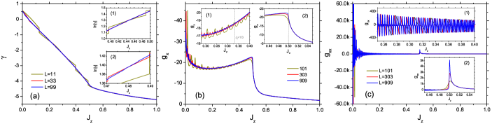
Figure 4: (Color online) (a) $\gamma$ curve along the selected variation path $J_{x}=J_{y}$ for $L=11,$ $33,$ and $99$. Both insets reveal the increasing number of saltation in $B$ phase proportional to the system size parameter $L$. (b) $g_{x}$ and (c) $g_{xx}$ as a function of $J_{z}$ along the variation path $J_{x}=J_{y}$ for system size parameters $L=101,303$ and $909$. The two insets are local enlarged-pictures, which show the vibration in $B$ phase and the circumstances in the critical point respectively.

It is meaningful to consider the first-order partial derivative $g_{{}_{\beta}}=\partial\gamma/\partial J_{\beta}$ ($\beta=x,y$) of the GP $\gamma$. Since the GP $\gamma$ in Eq. (19) is symmetric with respect to $J_{x}$ and $J_{y}$, we only need to investigate $g_{x}$ (or equivalently $g_{y}$). The variation of $g_{x}$ with respect to $J_{z}$ along the selected path of $J_{x}=J_{y}$ from $B$ phase to $A$ phase is shown in Fig. 4(b) for different system-size parameters $L=101$, $303$ and $909$. It can be seen from Fig. 4(b) that $g_{x}$ oscillates in $B$ phase with frequency (or number of peaks), which is proportional to $L$ (see inset (1) of Fig. 4(b)). This rapid variation of the GP $\gamma$ (in the $B$ phase) has not yet been found, to our knowledge. However, a very similar behavior of fidelity susceptibility in the Kitaev model has been reported S. Yang . On the other hand, the value of $g_{x}$ at the critical point $J_{z}=1/2$ increases with the system-size and sharply decays in $A$ phase (see inset (2) of Fig. 4(b) for detail). It is interesting to remark that the saltation of GP $\gamma$ in $B$ phase due to the complex structure of ground state with degeneracy (Fig. 2 (b),(c),(d)) is not random rather has regulation, especially it tends to a regular oscillation above the point, $J_{z}=1/3$ , (see inset (1) of Fig. 4(b)). The oscillation frequency depends linearly on the system size.

To show the non–analyticity of GP at the critical points explicitly the second-order derivative $g_{xx}$ of the GP $\gamma$ with respect to the coupling parameters is calculated. Fig. 4(c) shows the variation of $g_{xx}$ with respect to $J_{z}$ along the variation path of $J_{z}=J_{y}$ for different system-size parameters $L=101$, $303$ and $909$. Inset (1) reveals the increase of peak-number of $g_{xx}$ in $B$ phase along with the system-size $L$ similar to $\gamma$ and $g_{x}$ in behavior. The second-order derivative $g_{xx}$ is divergent at the critical point $J_{z}=1/2$ as shown in inset (2) indicating that the TQPT of the Kitaev honeycomb model is a second-order transition, While the QPT of the XY spin chain Zhu ; Zhu08 and the Dicke model Zhu08 ; Chen has been shown to be the first-order transition with the divergent first-order derivative of the GP. We conclude that the non-analytic GP $\gamma$ can very well describe the TQPT in terms of the Landau phase-transition theory.

Similarly, we can also choose the variation path as $J_{z}=1/4$ (dashed line in Fig. 1(b)) with two critical points $J_{x}=1/4$ and $J_{x}=1/2$. Qualitatively similar results are shown in Fig. 5 for different size parameters $L=101$ (red line), $303$ (blue) and $707$ (dark), respectively, where $\gamma$-plot is a smooth curve in $A$ phase for $J_{x}<1/4$ or $J_{x}>1/2$ and becomes saltant in $B$ phase when $1/4<J_{x}<1/2$ (Fig. 5(a)). The plots of $g_{x}$ and $g_{xx}$ are respectively shown in Fig. 5(b) and (c) displaying the clear vibration in the $B$ phase. $g_{x}$ has a sharp peak at the critical points and $g_{xx}$ is divergent in the thermodynamic limit showing the characteristic of second-order phase transition. Inset of Fig. 5(c) shows the detail of the vibration in the $B$ phase with the peak-number proportional to the system size.

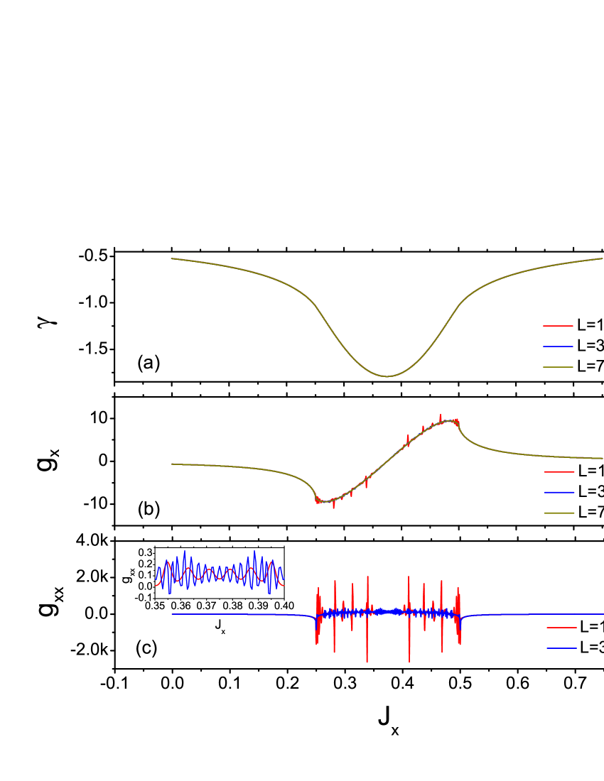
Figure 5: (Color online) (a) $\gamma$ curve, which is smooth in $A$ phase and saltant in $B$ phase, (b) $g_{x}$ curve and (c) $g_{xx}$ as a function of $J_{x}$ for $J_{x}$ varying along the path $J_{z}=1/4$, with critical points at $J_{x}=1/4$ and $J_{x}=1/2$.

IV Finite-size scaling

In order to quantify the non-analytic nature of GP through the critical points, and to further understand the quantum criticality, we investigate the scaling behavior of the GP and its first-order and second-order derivatives by the finite size scaling analysis Barber . Since the GP of a many-body system is an extensive quantity, it usually depends on the system size in the non-critical region. In the vicinity of critical point ($J_{z}^{C}=1/2$ here), the GP $\gamma$ follows a power lawLin

$$\gamma\propto{\left|J_{z}-J_{z}^{C}\right|}^{-\alpha_{\gamma}}$$ (20)

with $\alpha$ being corresponding exponent. ${\left|J_{z}-J_{z}^{C}\right|}$-dependence of $\gamma$ in the left-hand side of critical point ( $J_{z}<J_{z}^{C}$ ) and right-hand side ( $J_{z}>J_{z}^{C})$ is respectively plotted in Fig. 6(a) and (b) for different system-size parameters $L=101$, $303$ and $909$. The corresponding exponents $\alpha_{\gamma}^{-}=-0.99934\pm 0.00033$ (left-hand side) and $\alpha_{\gamma}^{+}=-0.83538\pm 0.00008$ (right-hand side) are obtained from Fig. 6(a) and (b). Similarly, $g_{x}$ and $g_{xx}$ as a function of $|J_{z}-J_{z}^{C}|$ are plotted in Fig. 6(c), (d) and (e), (f) for the gapless and gapped phases respectively, from which the critical exponents $\alpha_{g_{x}}^{-}=-0.17529\pm 0.02056$, $\alpha_{g_{xx}}^{-}=1.32523\pm 0.01719$ (left) for B phase and $\alpha_{g_{x}}^{+}=-0.48375\pm 0.00033$, $\alpha_{g_{xx}}^{+}=0.60687\pm 0.00526$ (right) for A phase are found. The fact of negative exponents $\alpha_{\gamma}^{\pm}$, $\alpha_{g_{x}}^{\pm}$ and positive $\alpha_{g_{xx}}^{\pm}$ indicates that $\gamma$ and $g_{x}$ are finite while $g_{xx}$ is divergent at the critical point in the thermodynamic limit. Thus the TQPT is a second-order phase transition characterized by the GP $\gamma$.

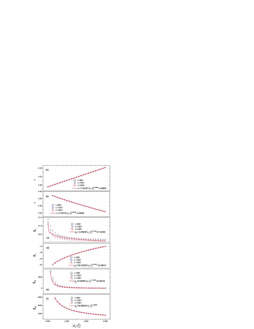
Figure 6: (Color online) Finite-size scaling analysis of the power-law divergence for (a) GP $\gamma$, (c) $g_{x}$, (e) $g_{xx}$ as a function of $|J_{z}-J_{z}^{C}|$ in the vicinity of critical point with system sizes $L=301,901$ and $1501$ on the left-hand side ($J_{z}<J_{z}^{C}$) and (b), (d), (f) on the right-hand side ($J_{z}>J_{z}^{C}$) respectively.

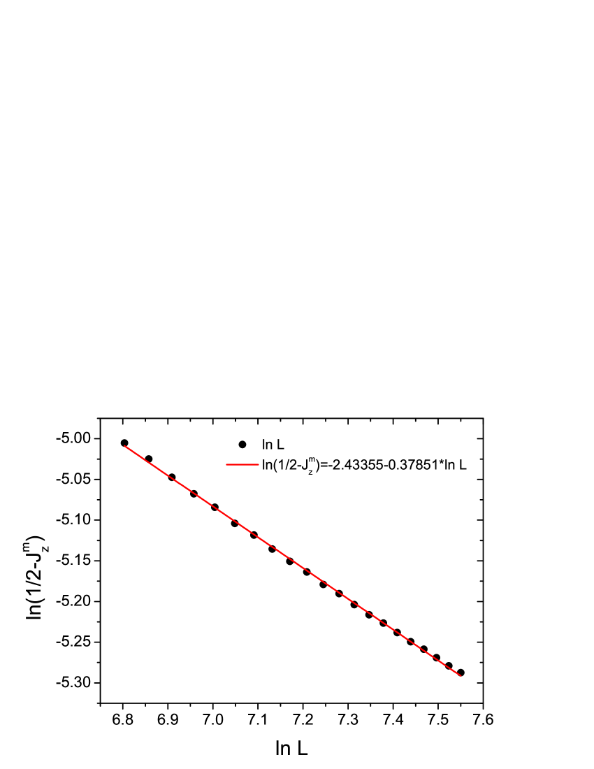
Figure 7: (Color online) $L$-dependence of $J_{z}^{C}-J_{z}^{m}$ in logarithmic coordinate for $L=901,951,...,1901$.

The position of maximum value of $\gamma$ denoted by $J_{z}^{m}$ may not be located exactly at the critical point $J_{z}^{C}=1/2$, but tends to it in the thermodynamic limit $L\rightarrow\infty$, which is regarded as the pseudocritical point Barber . The $J_{z}^{C}-J_{z}^{m}$ versus different system-size $L=901,951,...,1901$ in a logarithmic coordinate is plotted in Fig. 7, which is a straight line of slope $-0.37851\pm 0.00226$. It means that the $J_{z}^{m}$ tends toward to the critical point $J_{z}^{C}$ following the power-law decay

$$J_{z}^{C}-J_{z}^{m}\propto L^{-0.37851}.$$ (21)

On the other hand, the maximum value of $\gamma$ at $J_{z}=J_{z}^{m}$ for a finite-size system behaves as

$$\gamma({J_{z}^{m}})\propto{L}^{\mu_{\gamma}},$$ (22)

which is shown in the inset of Fig. 8(a) with a straight line in logarithmic coordinate. The corresponding size-exponent is given by $\mu_{\gamma}=0.01148\pm 0.00054$.

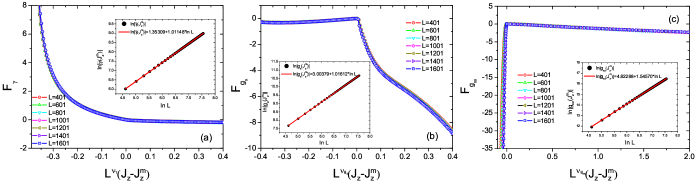
Figure 8: (Color online) (a) $F_{\gamma}$, (b) $F_{g_{x}}$, and (c) $F_{g_{xx}}$ as a function of $L^{\nu}\left(J_{z}-J_{z}^{m}\right)$ for $L=401,601,...,1601$. All the data fall on to a single curve respectively. And the three insets in turn shows the variation of $\gamma(J_{z}^{m})$, $g_{x}(J_{z}^{m})$, and $g_{xx}(J_{z}^{m})$ with respect to the system size-parameters $L=101,151,...,1901$.

Since the GP $\gamma$ around its maximum position $J_{z}^{m}$ can be written as a simple function of $J_{z}^{m}-J_{z}$, it is possible to make all the value-data defined by a universal scaling function $F_{\gamma}=\left({\gamma}({J_{z}^{m}})-\gamma\right)/\gamma$ versus $L^{\nu_{\gamma}}\left(J_{z}-J_{z}^{m}\right)$, namely,

$$F_{\gamma}=f\left[L^{\nu_{\gamma}}\left(J_{z}^{m}-J_{z}\right)\right],$$ (23)

where $\nu_{\gamma}$ is a critical exponent that governs the divergence of the correlation length. The values of $F_{\gamma}$ for different system-size parameters $L$ fall onto a single curve as shown in Fig. 8(a), from which we can extract the critical exponent $\nu_{\gamma}=-0.015$ numerically.

In fact, according to the scaling ansatz of a finite system Barber ; Lin , the critical exponent $\nu$ can be determined by the relation $\nu=\mu/\alpha$. In terms of this relation, the critical exponents in $B$ and $A$ phases are found as ${\nu}_{\gamma}^{-}=-0.01149$ and ${\nu}_{\gamma}^{+}=-0.01374$, which are consistent with the numerical result $\nu_{\gamma}$ extracted from Fig. 8(a). Inset of Fig. 8(b) is a plot of the maximum value of $g_{x}({J_{z}^{m}})$ as a function of $L$

$$g_{x}({J_{z}^{m}})\propto{L}^{\mu_{g_{x}}}$$ (24)

in logarithmic coordinate, from which the size exponent $\mu_{g_{x}}=0.01612\pm 0.00094$ is found. The universal scaling function

$$F_{g_{x}}=f\left[L^{\nu_{g_{x}}}(J_{z}^{m}-J_{z})\right]$$ (25)

is shown in Fig. 8(b). We have the numerical value $\nu_{g_{x}}=-0.040$ and the results determined by the relation $\nu=\mu/\alpha$ that $\nu_{g_{x}}^{-}=-0.09196$, $\nu_{g_{x}}^{+}=-0.03332$. The deviation between $\nu_{g}$ and $\nu_{g_{xx}}^{-}$ may be due to the rapid oscillation in the gapless $B$ phase. Similarly, the critical exponents of $g_{xx}$ can be obtained from Fig. 8(c) as $\mu_{g_{xx}}=0.54570\pm 0.00237$, $\nu_{g_{xx}}^{-}=0.410$ and $\nu_{g_{xx}}^{+}=0.908$, and the results determined by $\nu=\mu/\alpha$ are $\nu_{g_{xx}}^{-}=0.41178$ and $\nu_{g_{xx}}^{+}=0.89920$ respectively.

V Summary and discussion

We demonstrate that the ground-state GP generated by the correlated rotation of two linked-spins in a unit-cell indeed can be used to characterize the TQPT for the Kitaev honeycomb model. The non-analytic GP with a divergent second-order derivative at the critical points shows that the TQPT is a second-order phase-transition different from the $XY$ spin-chain Zhu ; Zhu08 , in which the first-order derivative of GP is divergent, and the LMG modelZhu ; Zhu08 , in which the GP itself is shown to be divergent. Moreover it is found that the GP is zigzagging with oscillating derivatives in the gapless $B$ phase, but is a smooth function in the gapped $A$ phase. The scaling behavior of the non-analytic GP in the vicinity of critical point is shown to exhibit the universality with negative exponents of both $\gamma$ and $g_{x}$ while a positive exponent of $g_{xx}$ indicating the characteristic of second-order phase transition.

References

- (1) Berry M V 1985 Proc. R. Soc. London, Ser. A 392 45
- (2) Berry M V 1990 Phys. Today 43 34
- (3) Shapere A and Wilczek F (Eds.) 1989 Geometric Phases in Physics (Singapore: World Scientific)
- (4) Bohm A, Mostafazadeh A, Koizumi H, Niu Q and Zwanziger J 2003 The Geometric Phase in Quantum Systems (New York: Springer)
- (5) Carollo A C M and Pachos J K 2005 Phys. Rev. Lett. 95 157203
- (6) Zhu S L 2006 Phys. Rev. Lett. 96 077206
- (7) Hamma A 2006 arXiv:quant-ph/0602091v1
- (8) Zhu S L 2008 Int. J. Mod. Phys. B 22 561
- (9) Chen G, Li J and Liang J-Q 2006 Phys. Rev. A 74 054101
- (10) Ma Y-Q and Chen S 2009 Phys. Rev. A 79 022116; Hirano1 T, Katsura1 H and Hatsugai Y 2008 Phys. Rev. B 77 094431; Richert J 2008 Phys. Lett. A 372 5352; Nesterov A I and Ovchinnikov S G 2008 Phys. Rev. E 78 015202(R); Basu B 2010 Phys. Lett. A 374 1205
- (11) Sachdev S 1999 Quantum Phase Transitions (England: Cambridge University Press)
- (12) Sondhi S L, Girvin S M, Carini J P and Shahar D 1997 Rev. Mod. Phys. 69 315
- (13) Tsui D C, Stormer H L and Gossard A C 1982 Phys. Rev. Lett. 48 1559
- (14) R. B. Laughlin 1983 Phys. Rev. Lett. 50 1395
- (15) Kitaev A 2003 Ann. Phys. (N.Y.) 303 2
- (16) Wen X G 2003 Phys. Rev. Lett. 90 016803
- (17) Yu J, Kou S P and Wen X G 2008 Europhys. Lett. 84 17004
- (18) Kitaev A 2006 Ann. Phys. (N.Y.) 321 2
- (19) Wen X G 2004 Quantum Field Theory of Many-Body Systems (Oxford: Oxford University Press)
- (20) Feng X Y, Zhang G M and Xiang T 2007 Phys. Rev. Lett. 98 087204
- (21) Jiang H C, Weng Z Y and Xiang T 2008 Phys. Rev. Lett. 101 090603
- (22) Chen H D and Hu J P 2007 Phys. Rev. B 76 193101
- (23) Chen H D and Nussinov Z 2008 J. Phys. A 41 075001
- (24) Yang S, Gu S J, Sun C P and Lin H Q 2008 Phys. Rev. A 78 012304
- (25) Gu S J 2010 Int. J. Mod. Phys. B 24 4371
- (26) Nayak C, Simon S H, Stern A, Freedman M and Sarma S D 2008 Rev. Mod. Phys. 80 1083
- (27) Liang J-Q and Müller-Kirsten H J W 1992 Ann. Phys. 219 42
- (28) Barber M N in: Domb C and Lebowitz J L (Eds.) 1983 Phase Transition and Critical Phenomena, vol. 8, pp. P145 (New York: Academic)
- (29) Gu S J, Kwok H M, Ning W Q and Lin H Q 2008 Phys. Rev. B 77 245109