Thomson and Compton scattering with an intense laser pulse

Abstract

Our paper concerns the scattering of intense laser radiation on free electrons and it is focused on the relation between nonlinear Compton and nonlinear Thomson scattering. The analysis is performed for a laser field modeled by an ideal pulse with a finite duration, a fixed direction of propagation and indefinitely extended in the plane perpendicular to it. We derive the classical limit of the quantum spectral and angular distribution of the emitted radiation, for an arbitrary polarization of the laser pulse. We also rederive our result directly, in the framework of classical electrodynamics, obtaining, at the same time, the distribution for the emitted radiation with a well defined polarization. The results reduce to those established by Krafft et al. [G. A. Krafft, A. Doyuran and J. B. Rosenzweig, Phys. Rev. E 72, 056502 (2005)] in the particular case of linear polarization of the pulse, orthogonal to the initial electron momentum. Conditions in which the differences between classical and quantum results are visible are discussed and illustrated by graphs.

I Introduction

The invention of the laser fifty years ago, has fostered many theoretical studies Eberly , treating the interaction of the electrons with an intense electromagnetic field. For theorists this was a field where new methods of investigation were necessary. Based on these, processes such as electron reflection and refraction, nonlinear Compton scattering and one-photon pair production have been studied. In recent years, progress of experimental physics, leading to the detection of some of the fundamental nonlinear processes possible in head-on collisions of very fast electrons with an intense laser beam (10¹⁸ W/cm²) SLAC , has renewed interest in theoretical studies, especially in the relativistic regime. Review papers such as those of Salamin et al. Hatz and Ehlotzky et al. EKK have been published and we refer to them for bibliography and details.

The particular new interest for nonlinear Compton scattering with free electrons is also related to the possibility it opens for new sources of ultra short pulses in the X-ray domain, with durations extending from the picosecond range, as discussed by Esarey et al. Esarey , to the attosecond domain as . Even the production of zeptosecond X-ray pulses is under theoretical study LLCW . Envisaged applications are numerous and various and they continue to stimulate experimental investigations Bab .

In the description of intense radiation scattering on free electrons, classical electrodynamics (CED), in which the electron is subject to the laws of classical mechanics and the electromagnetic field obeys Maxwell equations, as well the theory applying quantum mechanics for the electron, are used in the literature. In the latter case, the external field is described classically but, as the process involves spontaneous emission of a photon, the interaction with the quantized electromagnetic field is also taken in account. This hybrid approach will be referred to as quantum in the following.

In the regime of low incident radiation frequency $\,\omega_{1}\,$, such that $\,\hbar\omega_{1}\ll mc^{2}\,$ ($m$ the electron mass and $c$ the velocity of light), the name Thomson scattering is currently given to the process. In this situation, classical theory is used and so under the name of nonlinear Thomson scattering one finds classical calculations. And then one speaks sometimes in the literature about ”the transition from Thomson to Compton scattering” MKM . We shall adhere to this terminology in our paper, using Compton’s name when referring to quantum calculations and Thomson’s name for classical calculations.

The majority of published calculations, classical or quantum, refer to the monochromatic case. With some exceptions that illuminate the analysis of the laser pulse case, we shall not quote them here, as they are well described in the review papers we have mentioned before.

The subject of our paper is the connection between Thomson and Compton scattering beyond the monochromatic case. Our study is performed for an electromagnetic plane wave which is supposed to have a finite extension in the direction of propagation but an indefinite extension in the plane orthogonal to this direction. This wave will be designated in the following as a laser pulse. Our contribution concerns two aspects: i) the connection between the basic equations describing Thomson and Compton scattering and ii) qualitative and quantitative similarities and differences in the predictions extracted from these equations.

For Thomson scattering with a laser pulse, alternative expressions to the general ones found in the textbooks Jks for the energy and angular distribution of the emitted radiation have been derived by Krafft Krf1 ; Krf2 in a particular scattering geometry. The evolution of the classical electron in the case of a plane wave and beyond it is discussed in detail by Hartemann and coworkers Hart3D in their paper presenting calculations based on an accurate description of the three-dimensional focus of a laser wave, in both the near-field and far-field regions; more papers presenting numerical calculations for a realistic, focused laser pulse have been published in the last ten years (Lee et al. cor , Gao Gao , Lan et al. Lan , Heinzl et al. UK-nou ). Other numerical calculations Hartpro have investigated different aspects such as the effects of the electron beam emittance and energy spread on the emitted spectrum. More subtle effects as radiation damping are studied HG .

Although elaborated many years ago, quantum theory have been applied less to this problem and almost all the calculations refer only to an electromagnetic plane wave, taking advantage of the existence of the Volkov solutions of the Dirac equation. Several recent extended calculations have been made for the monochromatic case UK ; HI and some others for the laser pulse case Fofa ; BF ; UK-nou . A quantum calculation that goes beyond the electromagnetic plane wave model for the laser beam and the description by Volkov solutions is that of Krekora et al. Krekora . They have solved the time-dependent Dirac equation for an electron wave packet accelerated by a very strong laser field and have used the Lienard-Wiechert solution of Maxwell equations in order to calculate the scattered light spectra. In particular, they have shown that the width of the initial electronic wavepacket influences the spectrum. More recently, the emission by an electron described by a wavepacket was studied by Peatross et al. wpk , with the conclusion that ”the radiative response can be mimicked by the incoherent emission of a classical ensemble of point charges”.

Generally, it is expected that the CED results are good when the electron energy loss is small, such that its effect on the electron motion is negligible. This situation was already exploited decades ago by Kramers Kramers in a study of electron bremsstrahlung in a Coulomb field and leads to results close to those given by quantum theory RHP for small kinetic energy $\,T_{1}\,$ of the electron, $\,T_{1}\ll\alpha^{2}\,Z^{2}\,,$ with $\,\alpha\,$ the fine structure constant and $\,Z\,$ the nuclear charge.

The connection between quantum and CED results has been discussed in the literature in the monochromatic case. In particular, Goreslavskii et al. GRSL have derived the classical energy and angular distribution of radiation starting from the quantum results, in the case of circularly polarized monochromatic radiation. They formulate conditions of applicability of the classical limit for weak fields and for very intense fields. Very recent papers comparing Thomson and Compton scattering are those of Hartemann Hart and Heinzl et al. UK-nou . In UK-nou the comparison is made using numerical data obtained from both classical and quantum calculations for the particular conditions relevant to experiments planned at the Forschungszentrum Dresden-Rossendorf (FZD) and a set of realistic parameters is proposed for an experiment allowing the detection of non-linear Thomson scattering to be performed.

New features of Compton scattering at intensities of the order 10¹⁸W/cm² and very energetic electrons (GeV range) have been revealed by recent studies Heinzl . At intensities above 10²²W/cm² predictions are that QED effects will modify the radiation emission from these electrons Sokol .

Our paper is organized as follows. At the beginning of Sect. II we describe the theoretical framework in which our study is performed and the equations we use in several analytic calculations in both quantum (Sect. II A) and classical (Sect. II B) treatments. In Sect. III we present, for the case of a laser pulse, the derivation of an alternative expression (35) to the standard one [Eq. (14.65) of Jackson’s book Jks ] for the energy and angular distribution of the emitted radiation. This expression is derived as the classical limit of the quantum expression (14). Based on the calculation in Appendix B, made in the framework of CED, we present the classical radiation distributions for two particular state of polarizations. Our formulas are valid for any polarization of the laser; for the particular case of linear polarization orthogonal to the direction of the incident electron they reduce to the expressions published by Krafft et al. Krf2 which are valid only for this configuration. Sections IV and V are devoted to the comparison between classical and quantum calculations. While qualitative aspects are discussed in Sect. IV implying also the monochromatic case, in Sect. V the comparison is quantitative and it is made with the aim of revealing situations in which the differences matter.

The formulae are given in S.I. units. Numerical results for photon distributions are presented in atomic units, but photon energies are given in eV. The equations in Appendix A for the classical electron trajectory are used in Sect. II in the passage from quantum to classical distributions and in Appendix B, where the new version of the classical distribution is derived directly from Eq. (14.65) of Jackson’s textbook Jks .

II Theoretical background

Compton scattering is the name primarily associated with the interaction of a free electron and a photon leading to the emission of a photon with a different direction and frequency (inelastic scattering) and the recoil of the electron. Energy and momentum are conserved and this leaves undetermined two of the six variables of the problem (final photon and electron momenta). This picture, implying the photon, is justified in QED, using second-order perturbation theory, and is suitable at low intensities of the external field. Quantum theory also describes the case in which the electromagnetic field is intense, when perturbation theory is not applicable. In this case the theory adopts a hybrid approach, describing the electron within quantum mechanics (Dirac equation), the external electromagnetic field within CED, and also takes into consideration the interaction of the electron with the quantized electromagnetic field which is responsible for spontaneous photon emission. One can single out the rate for the emission of only one photon in the interaction of the electron with the two electromagnetic fields.

In the following the external field is a plane wave with a fixed direction of propagation characterized by a unity vector $\,{\bf n}_{1}\,,$ with a finite extension in the direction of propagation and indefinitely extended in the transverse plane. The initial electron momentum is denoted by $\,{\bf p}_{1}\,$. The final electron has a momentum denoted by $\,{\bf p}_{2}\,$ and the emitted photon has the frequency $\,\omega_{2}\,$ and the propagation direction along the unity vector $\,{\bf n}_{2}\,$.

A basic quantity predicted by quantum theory is the radiated energy distribution over frequency and direction of the emitted photon and over the momentum of the scattered electron

$$d^{4}\,W=\rho_{4}(\omega_{2},{\bf n}_{2},{\bf p}_{2})\,d\omega_{2}\,d\Omega_{2}\,d{\bf p}_{2}\,.$$ (1)

We refer to the case in which an average and a summation over the initial and final electron spin was made, and a summation over the emitted photon polarization as well. If the scattered electron is not observed, the relevant quantity is

$$d^{2}\,W=\rho_{2}(\omega_{2},{\bf n}_{2})\,d\omega_{2}\,d\Omega_{2}\,,\qquad\rho_{2}(\omega_{2},{\bf n}_{2})=\int_{{\bf p}_{2}}\rho_{4}(\omega_{2},{\bf n}_{2},{\bf p}_{2})\,d{\bf p}_{2}\,.$$ (2)

In CED formalism, the electron, accelerated by the field, emits radiation. The theory leads to predictions for this radiation. The calculation we refer to is made with the assumption that the emission of radiation does not affect the particle motion, so the electron moves on a trajectory well determined by the initial conditions and the final electron momentum is well determined. As a consequence one is led only to a distribution of the emitted radiation frequency and direction,

$$d^{2}\,W^{\mathrm{cl}}=\rho_{2}^{\mathrm{cl}}(\omega_{2},{\bf n}_{2})\,d\omega_{2}\,d\Omega_{2}\,.$$ (3)

From the distribution $\,d^{2}W/d\omega_{2}\,d\Omega_{2}\,$ one obtains, in either the classical or the quantum case, the angular distribution of the radiated energy $\,dW/d\Omega_{2}\,$, its frequency distribution $\,dW/d\omega_{2}\,$ and the total emitted energy $\,W_{\mathrm{total}}\,$.

The external field we consider is described by a vector potential $\,{\bf A}\,$ orthogonal to the direction of propagation ${\bf n}_{1}$ and depending only on the variable

$$\phi=t-{\bf r}\cdot{\bf n}_{1}/c\,.$$ (4)

We shall use the four-vectors

$$n_{1}=(1,{\bf n}_{1})\,,\qquad\widetilde{n}_{1}=(1,-{\bf n}_{1})\,,\qquad n_{1}^{2}=\widetilde{n}_{1}^{2}=0\,,\qquad n_{1}\cdot\widetilde{n}_{1}=2\,,$$ (5)

so $\,\phi=n_{1}\cdot x/c\,$, where $\,x=(ct,{\bf r})\,$ is the position four-vector. In the monochromatic case the vector potential $\,{\bf A}\,$ is a periodic function of $\,\phi\,$, while in the laser pulse case it could be an arbitrary function of it, which becomes negligible for values of $\,\phi\,$ outside a finite range $\,(\phi_{\mathrm{in}},\phi_{\mathrm{f}})\,$. This implies that at fixed position $\,{\bf r}\,$ the external field is present a finite duration, equal to $\,\phi_{\mathrm{f}}-\phi_{\mathrm{in}}$. We denote by $\,A_{0}\,$ the maximum value taken by the vector potential and use the notation

$$\eta\equiv\frac{\mid e\mid A_{0}}{mc}\,,$$ (6)

with $\,e<0\,$ the electron charge. In the monochromatic case the dimensionless quantity $\,\eta^{2}\,$ is directly proportional to the intensity of the wave and inversely proportional to the square of the frequency.

II.1 The radiated energy distribution in quantum theory

As mentioned before, in the approach we use here, the external field is described classically; the electron, described in quantum mechanics, interacts also with the quantized electromagnetic field and this interaction, treated in first-order perturbation theory, leads to spontaneous emission of radiation.

Owing to the existence of the Volkov spinors, exact solutions of the Dirac equations for the electron in a classical electromagnetic plane wave, which reduce to plane wave spinors in the absence of the field, one can write an analytic expression for the transition amplitude. Its expression in the monochromatic case is given in many papers, starting with those from 1964, as quoted for instance in EKK . For the case of a pulse, the transition amplitude is proportional to a product of $\,\delta$-functions

$${\cal T}\sim\,\delta({\bf p}_{1\perp}-{\bf p}_{2\perp}-\hbar{\bf k}_{2\perp})\,\delta[n_{1}\cdot(p_{1}-p_{2}-\hbar k_{2})]\,,$$ (7)

where the index $\,\perp\,$ indicates the components orthogonal to the direction of propagation of the laser pulse ${\bf n}_{1}$, taken in the following as the $Oz$ axis. The function that multiplies the $\,\delta$-functions can be expressed in terms of three integrals BF . Details will given in what follows.

As a consequence of the $\,\delta$-functions present in (7), three conservation laws are valid in the case of a laser pulse. They completely determine the value of the momentum $\,{\bf p}_{2}\,$, for fixed emitted photon frequency and direction. According to Eq. (40) of BF , this momentum, denoted by $\,\widetilde{\bf p}_{2}\,$, has the spatial components

$$\widetilde{\bf p}_{2\perp}={\bf p}_{1\perp}-\hbar{\bf k}_{2\perp},\qquad\widetilde{p}_{2z}=\frac{(mc)^{2}+({\bf p}_{1\perp}-\hbar{\bf k}_{2\perp})^{2}}{2n_{1}\cdot(p_{1}-\hbar k_{2})}-\frac{n_{1}\cdot(p_{1}-\hbar k_{2})}{2}\,\,$$ (8)

and the temporal component

$$\widetilde{p}_{2}^{0}=\sqrt{(mc)^{2}+\widetilde{\bf p}^{2}}=\frac{(mc)^{2}+({\bf p}_{1\perp}-\hbar{\bf k}_{2\perp})^{2}}{2n_{1}\cdot(p_{1}-\hbar k_{2})}+\frac{n_{1}\cdot(p_{1}-\hbar k_{2})}{2}\,.$$ (9)

The conservation law for the momentum components perpendicular to $\,{\bf n}_{1}\,$ is the same as in the monochromatic case.

The three 1D $\delta$-functions are also present in the transition probability. Integration over the electron attributes eliminates them. In order to obtain the probability for the emission of a photon with the frequency in $(\omega_{2},\omega_{2}+d\omega_{2})\,$ and direction in the solid angle element $\,d\Omega_{2}\,$, we can directly use Eqs. (42) in BF : we have to multiply the cross section $\,d^{2}\sigma_{\gamma}\,$ by the flux $\,J\,$ (as defined in Eq. (33) of the quoted paper) and by the effective duration of the pulse $\,\widetilde{\tau}_{p}\,$. We also have to include the factor $\,\widetilde{p}_{2}^{\,0}/n_{1}\cdot\widetilde{p}_{2}\,$ omitted previously in BF . After that, the quantum radiated energy distribution is obtained by multiplying the transition probability with the energy of the emitted photon.

Here we write the spectrum in terms of the integrals $\,{\bf a}^{(q)}\,$ (already used in BF , and denoted there by  ${\cal{A}}$ ), and the integral $\,{b}^{(q)}\,$ we introduce here. These integrals are

$${\bf a}^{(q)} = -\int\limits_{-\infty}^{\infty}\,d\phi\,\frac{e{\bf A}(\phi)}{mc}\,\exp[\,-{i}\,\Phi(p_{2},p_{1};\phi)\,]\,,\;\quad$$ (10)

$${b}^{(q)} = \int_{{-\infty}}^{\infty}\,d\phi\,\frac{e^{2}{\bf A}^{2}(\phi)}{2(mc)^{2}}\exp[\,-{i}\,\Phi(p_{2},p_{1};\phi)\,]\,,$$ (11)

with

$$\Phi(p_{2},p_{1};\phi)\equiv\frac{1}{\hbar}\,\left[\frac{c}{2}\,\phi\,\widetilde{n}_{1}\cdot(p_{1}-p_{2}-\hbar k_{2})+F(p_{1};\phi)-F(p_{2};\phi)\right]$$ (12)

and

$$F(p;\phi)=\frac{c}{2(n_{1}\cdot p)}\int\limits_{\phi_{0}}^{\phi}d\chi[e^{2}{\bf A}^{2}(\chi)-2e{\bf A}(\chi)\cdot{\bf p}_{\perp}]\,.$$ (13)

The integration in (10) and (11) extends in fact over the pulse duration. A change of the value of the arbitrary constant $\,\phi_{0}\,$ in (13) will lead to an over-all phase factor in the transition amplitude with no effect on the transition probability.

As a result of the integration over the electron momentum, in the expression of the photon spectral and angular distribution that follows, the four momentum $\,p_{2}\,$ has to be replaced with the four-momentum $\,\widetilde{p}_{2}\,$ described in (8). We write the mentioned distribution as

$$\frac{d^{2}W}{d\omega_{2}\,d\Omega_{2}}=\frac{e_{0}^{2}\omega^{2}}{4\pi^{2}c}\frac{(mc)^{2}}{(n_{1}\cdot\widetilde{p}_{2})^{2}}\frac{\widetilde{p}_{2}^{\,0}}{p_{1}^{\,0}}{\cal R}\,,$$ (14)

where

$${\cal R}=c_{1}\,|{\bf a}^{(q)}|^{2}+{c_{2}\,(mc)^{2}\vline\,\frac{{\bf a}^{(q)}\cdot{{\bf d}}}{{\bf n}_{1}\cdot{\bf P}}\,\vline}^{\,2}+c_{3}\,|b^{(q)}|^{2}+2\,c_{4}\,m\,c\,\Re\left((b^{(q)})^{*}\,\frac{{\bf a}^{(q)}\cdot{\bf d}}{{\bf n}_{1}\cdot{\bf P}}\right)\,,$$ (15)

with

$$c_{1} = 1+\frac{(\hbar k_{2}\cdot n_{1})^{2}}{2(mc)^{2}}\gamma_{11}\,,\qquad c_{2}=2\,{\bf n}_{1}\cdot{\bf P}\,\frac{c_{1}}{\gamma_{11}(n_{1}\cdot\hbar k_{2})}+c_{5}$$

$$c_{3} = (mc)^{2}\,\frac{d_{0}^{2}}{({\bf n}_{1}\cdot{\bf P})^{2}}\,c_{5}\,,\qquad c_{4}=d_{0}\,[\,\frac{mc}{n_{1}\cdot\hbar k_{2}}\frac{c_{1}}{\gamma_{11}}+\frac{mc}{{\bf n}_{1}\cdot{\bf P}}\,c_{5}\,]\,,$$ (16)

and

$$c_{5} = \left[-1+\left(\frac{1}{\gamma_{12}}+\frac{1}{\gamma_{21}}\right)\frac{1}{n_{1}\cdot n_{2}}\right],\quad\gamma_{ij}=\frac{(mc)^{2}}{(n_{i}\cdot p_{1})(n_{j}\cdot\widetilde{p}_{2})},\quad i,j=1,2$$ (17)

$${d}_{0} = m\,c\,\left(\frac{1}{n_{1}\cdot p_{1}}-\frac{1}{n_{1}\cdot\widetilde{p}_{2}}\right),\quad{\bf d}=\frac{{\bf p}_{1}}{n_{1}\cdot p_{1}}-\frac{\widetilde{\bf p}_{2}}{n_{1}\cdot{\widetilde{p}_{2}}},\quad{\bf P}={\bf p_{1}}-\widetilde{\bf p}_{2}-\hbar{\bf k}_{2}\;.$$ (18)

II.2 The classical energy and angular distribution

The most used equation for the distribution of the emitted photons over directions and frequencies is that derived in Jackson’s book [see Jks , Eq.(14.65)],

$$\frac{d^{2}W^{\mathrm{cl}}}{d\omega_{2}d\Omega_{2}}=2\,|{\bf K}(\omega_{2},{\bf n}_{2})|^{2}\,,$$ (19)

where

$${\bf K}(\omega_{2},{\bf n}_{2})=\frac{e_{0}}{2\pi\sqrt{2c}}\int\limits_{-\infty}^{\infty}\,\frac{dt}{\kappa^{2}}\,{\bf n}_{2}\times[({\bf n}_{2}-\bm{\beta})\times\dot{\bm{\beta}}]\,\exp[-i\Phi^{\mathrm{cl}}]\,,\qquad e_{0}^{2}\equiv\frac{e^{2}}{4\pi\epsilon_{0}}\,,$$ (20)

with $\,{\bf n}_{2}$ the unity vector of the observation direction and

$$\bm{\beta}(t)=\frac{{\bf v}(t)}{c}\,,\qquad\kappa=1-{\bf n}_{2}\cdot\bm{\beta}\,,\qquad\Phi^{\mathrm{cl}}=-\omega_{2}\,\left(t-\frac{{\bf n}_{2}\cdot{\bf r}(t)}{c}\right)\,.$$ (21)

In formula (20) the position $\,{\bf r}(t)\,$, the velocity and the acceleration of the moving electron are all implied.

If the electron is at rest at the initial and final moments in regions where the electromagnetic pulse is zero, an integration by parts leads to the simpler expression [Jackson’s Eq. (14.67)],

$${\bf K}(\omega_{2},{\bf n}_{2})=-{i}\,\frac{e_{0}}{2\pi\sqrt{2c}}\,\omega_{2}\,\int\limits_{-\infty}^{\infty}\,dt\;{\bf n}_{2}\times({\bf n}_{2}\times\bm{\beta})\,\exp[-i\Phi^{\mathrm{cl}}]\,,$$ (22)

which requires only the electron position and velocity along its trajectory.

Equations (20) and (22) are valid for any external electromagnetic field. In the following we shall refer only to the case of a plane wave, when the only variable is $\,\phi\,$, defined in (4). In this case the expressions given in Appendix A for the trajectory and velocity are valid. We transcribe here the expression (21) of the classical phase $\,\Phi^{\mathrm{cl}}\,$, as convenient for further reference. First we write

$$\Phi^{\mathrm{cl}}=-\omega_{2}\,[\,\phi+({\bf n}_{1}-{\bf n}_{2})\cdot\frac{{\bf r}(t)}{c}\,]\,$$ (23)

and then, using the expressions of the vector $\,{\bf r}\,$, as a function of $\phi\,$ as in Eqs.(A), one obtains the phase in terms of the variable $\,\phi\,$. Starting from now, we shall use the notation $\,\Phi^{\mathrm{cl}}(p_{1};\phi)\,$ displaying also the argument $\,p_{1}\,$, but not $\,\omega_{2}\,$ and $\,n_{2}\,$, in order to have a reasonably simple notation, corresponding to that used in (12),

$$\Phi^{\mathrm{cl}}(p_{1};\phi)=-\omega_{2}\,[\,\phi\,\frac{n_{2}\cdot p_{1}}{n_{1}\cdot p_{1}}+\frac{n_{1}\cdot n_{2}}{2(n_{1}\cdot p_{1})^{2}}\,\int_{\phi_{0}}^{\phi}e^{2}{\bf A}^{2}(\chi)\,d\chi+{\bf W}\cdot\int_{\phi_{0}}^{\phi}\frac{e{\bf A}(\chi)}{mc}\,d\chi]+\Phi_{0}\,,$$ (24)

with

$${\bf W}\equiv mc\,\left(\frac{{\bf n}_{2}}{n_{1}\cdot p_{1}}-\frac{n_{1}\cdot n_{2}}{(n_{1}\cdot p_{1})^{2}}\,{\bf p}_{1}\right)\,.$$ (25)

$\,\Phi_{0}\,$ is a constant with respect to the integration variable $\,t\,$ in (20). It gives a constant phase factor which has no effect on the energy distribution.

A change of variable from $\,t\,$ to $\,\phi\,$ is useful and is described in Appendix B. The variable $\,\phi\,$ has already been used in the literature both in quantum and classical calculations BK ; Sa-Sa ; it was used in particular by Krafft et al. Krf1 ; Krf2 in their derivation of the energy distribution for two polarization states of the emitted photon, for a special initial configuration. In the next section, using a procedure different from that Krafft et al., we derive the same type of formula, but valid for any polarization of the laser and arbitrary initial directions of propagation of the laser and initial electron.

In CED, a general compact expression is valid for the angular distribution (Eq. (14.53) of Jks ), namely

$$\frac{dW^{\mathrm{cl}}}{d\Omega_{2}}=\frac{e_{0}^{2}}{4\pi c}\int\limits_{-\infty}^{\infty}\,\frac{dt}{\kappa^{5}}\,|\,{\bf n}_{2}\times[({\bf n}_{2}-{\bm{\beta}})\times\dot{\bm{\beta}}]\,|^{\,2}\,,$$ (26)

with $\,\kappa\,$ defined in (21). In fact, Jackson’s calculation Jks starts with the angular distribution of the radiation and from it derives its spectral decomposition. This means that going from Eq. (19) to Eq. (26), i.e., integrating over emitted frequencies, the interferences between the fields emitted at different times are destroyed. We have used Eq. (26) in the verification of our numerical codes.

III Alternative expression for the energy distribution of radiation emitted in Thomson scattering with a laser pulse

We present here how the classical energy distribution emerges from the quantum expression (14). That our equation (35) can be obtained also from the general formulas of CED is proven in Appendix B. At the end of this section we shall present the generalization of the analytic results derived previously by Krafft et al. Krf2 .

The classical limit can be obtained in a very formal way as the limit $\,\hbar\rightarrow 0\,$ of the quantum expression (14). The Planck constant appears explicitly, as $\,1/\hbar\,$ in the expression (12) of the phase, and through the emitted photon momentum $\,\hbar\,k_{2}$. We expect the classical approximation to be good if the emitted photon energy $c\hbar k_{2}$ is small with respect to the electron energy.

Firstly we analyze the phase (12). We need to consider the phase for the value $\,\widetilde{p}_{2}\,$ of the first argument, i.e., $\,\Phi(\widetilde{p}_{2},p_{1};\phi)\,$, with $\,\widetilde{p}_{2}\,$ given by (8) and (9). In this case one has

$$\widetilde{n}_{1}\cdot(p_{1}-\widetilde{p}_{2}-\hbar\,k_{2})=2\,{\bf n}_{1}\cdot{\bf P}\,$$ (27)

where $\,\widetilde{n}_{1}\,$ and $\,{\bf P}\,$ are defined in (5) and (17), respectively. The general expression (12) of the phase can then be directly transcribed as

$$\Phi(\widetilde{p}_{2},p_{1};\phi)=\frac{1}{\hbar}\,[\,c\phi\,{\bf n}_{1}\cdot{\bf P}+\frac{e^{2}}{2m}\,d_{0}\,\int_{\phi_{0}}^{\phi}\,d\chi\,{\bf A}^{2}(\chi)-ec\,{\bf d}\,\cdot\int_{\phi_{0}}^{\phi}\,d\chi\,{\bf A}(\chi)\,]\,,$$ (28)

with $\,d_{0}\,$ and $\,{\bf d}\,$ defined in (18). We keep only the terms linear in $\,\hbar k_{2}\,$ in $\,d_{0}\,$ and $\,{\bf d}\,$. It is easy to show that

$$c\,{\bf n}_{1}\cdot{\bf P} = -\hbar\,\omega_{2}\,\frac{n_{2}\cdot p_{1}}{n_{1}\cdot p_{1}}+{\cal O}(\hbar^{2})\,,\qquad d_{0}=-m\,\hbar\omega_{2}\frac{n_{1}\cdot n_{2}}{(n_{1}\cdot p_{1})^{2}}+{\cal O}(\hbar^{2})$$ (29)

$${\bf d}_{\perp} = \hbar\,[\,\frac{{\bf k}_{2\,\perp}}{n_{1}\cdot p_{1}}-\frac{n_{1}\cdot k_{2}}{(n_{1}\cdot p_{1})^{2}}\,{\bf p}_{1\,\perp}\,]+{\cal O}(\hbar^{2})=\frac{\hbar\,\omega_{2}}{mc^{2}}\,{\bf W}_{\perp}+{\cal O}(\hbar^{2})\,.$$ (30)

The vector $\,{\bf W}\,$ is the one defined in (25).

With the previous results, the comparison with (24) shows the expected behaviour:

$$\Phi(\widetilde{p}_{2},p_{1};\phi)=\Phi^{\mathrm{cl}}(p_{1};\phi)+{\cal O}(\hbar)\,.$$ (31)

In the integrals $\,{\bf a}^{(q)}\,$ and $\,b^{(q)}\,$ defined by (10) only the phase $\,\Phi\,$ is affected by the limit $\,\hbar\rightarrow 0\,$, so one has

$${\bf a}^{(q)} \rightarrow {\bf a}^{\mathrm{cl}}\equiv-\int_{-\infty}^{\infty}\,d\phi\,\frac{e{\bf A}(\phi)}{mc}\,\exp[-i\Phi^{\mathrm{cl}}(p_{1};\phi)]\,,$$ (32)

$$b^{(q)} \rightarrow b^{\mathrm{cl}}\equiv\int_{-\infty}^{\infty}\,d\phi\,\frac{e^{2}\,{\bf A}^{2}(\phi)}{2m^{2}c^{2}}\,\exp[-i\Phi^{\mathrm{cl}}(p_{1};\phi)]\,.$$ (33)

Using Eq. (29) in (16), one obtains the classical limit of the coefficients $c_{1},\ldots,c_{4}$:

$$c_{1}^{\mathrm{cl}}=1,\quad c_{2}^{\mathrm{cl}}=-1\,,\qquad c_{3}^{\mathrm{cl}}=c_{0}(2-c_{0})\,,\qquad c_{4}^{\mathrm{cl}}=1-c_{0}\,,\qquad c_{0}=\frac{(mc)^{2}(n_{1}\cdot n_{2})}{(n_{1}\cdot p_{1})(n_{2}\cdot p_{1})}.$$ (34)

Using the previous expressions we get from the quantum spectrum (14), the classical limit

$$\frac{d^{2}W^{cl}}{d\Omega_{2}\,d\omega_{2}} = \frac{e_{0}^{2}}{4\pi^{2}c}\,\omega_{2}^{2}\,\frac{(mc)^{2}}{(n_{1}\cdot p_{1})^{2}}\{\mid{\bf a}^{\mathrm{cl}}\mid^{2}-\frac{(n_{1}\cdot p_{1})^{2}}{(n_{2}\cdot p_{1})^{2}}\mid{\bf a}^{\mathrm{cl}}\cdot{\bf W}\mid^{2}$$ (35)

$$+ \,c_{3}^{\mathrm{cl}}\mid b^{\mathrm{cl}}\mid^{2}-2\,\frac{n_{1}\cdot p_{1}}{n_{2}\cdot p_{1}}c_{4}^{\mathrm{cl}}\,\Re[\left(b^{\mathrm{cl}}\right)^{*}\,{\bf a}^{\mathrm{cl}}\cdot{\bf W}\,]\,\}\,.$$

For an electron initially at rest, $\,{\bf p}_{1}=0\,$, one has $\,n_{1}\cdot p_{1}\rightarrow mc\,,\;n_{2}\cdot p_{1}\rightarrow mc\,,\;{\bf W}\rightarrow{\bf n}_{2}\,$ and the expression of the photon distribution has the simpler form

$$\frac{d^{2}\,W^{\mathrm{cl}}}{d\Omega_{2}\,d\omega_{2}}\rightarrow\frac{e_{0}^{2}}{4\pi^{2}\,c}\,\omega_{2}^{2}\,\left(\mid{\bf a}^{\mathrm{cl}}\mid^{2}-\mid{\bf a}^{\mathrm{cl}}\cdot{\bf n}_{2}\mid^{2}+\sin^{2}\theta\mid b^{\mathrm{cl}}\mid^{2}-2\,\cos\theta\,\Re[\left(b^{\mathrm{cl}}\right)^{*}\,{\bf a}^{\mathrm{cl}}\cdot{\bf n}_{2}\,]\right)\,,$$ (36)

with $\,\theta\,$ the photon scattering angle, $\,{\bf n}_{1}\cdot{\bf n}_{2}=\cos\theta\,$.

Equation (35), with the coefficients defined in (34), represents our final compact formula for the classical spectral and angular distribution in the case of scattering of an external electromagnetic plane wave with arbitrary polarization on a free electron.

As mentioned in Sect. I, for linear polarization of the pulse, orthogonal to the electron initial momentum the same type of formula as (35) was established by Krafft et al Krf1 ; Krf2 , by a completely different procedure. Defining the scattering plane as the plane containing the vectors $\,{\bf p}_{1}\,$ and $\,{\bf n}_{1}\,$, these authors start with the radiation spectrum decomposed into the contribution of polarization perpendicular ($\sigma$) and polarization parallel ($\pi$) to the plane of scattering in the reference system in which the electron is at rest; then they use an appropriate Lorentz transformation to describe the case of an initially moving electron. Their final results are contained in Eqs. (14-16) of Krf2 . We compared our final result (35), taken for a linearly polarization pulse with $\,{\bf A}\cdot{\bf p}_{1}=0$, and the sum of the contributions of the two polarizations, as given by the quoted authors. Agreement was found, except for the extra factor 1/2 that Krafft et al. use and explain after their Eq. (1).

The derivation we presented for Eq. (35) was simple, but it is based on knowledge of the quantum spectrum. The question arises how this formula emerges from the general equation (20) of CED. We give the answer in Appendix B, where the expression (20), valid for an electron with an initial velocity different of zero, is transformed in the case of a pulse. Our final result, justified in Appendix B, expresses the vector $\,{\bf K}\,$ by the simpler vector $\,{\bf K}_{0}\,$, as

$${\bf K}={\bf n}_{2}\times({\bf n}_{2}\times{\bf K}_{0})\,,$$ (37)

where

$$\qquad\qquad{\bf K}_{0}=-i\,\frac{e_{0}}{\pi\sqrt{8c}}\frac{mc}{n_{1}\cdot p_{1}}\omega_{2}\,[\,{\bf a}^{\mathrm{cl}}+t_{1}\,{\bf n}_{1}+t_{2}\,\frac{{\bf p}_{1}}{mc}\,]\,.$$

$$t_{1}=\frac{mc}{n_{1}\cdot p_{1}}\left(b^{\mathrm{cl}}+\frac{{\bf a}^{\mathrm{cl}}\cdot{\bf p}_{1}}{mc}\right)\,,\qquad t_{2}=-\frac{n_{1}\cdot p_{1}}{n_{2}\cdot p_{1}}\,[\,\left(\frac{mc}{n_{1}\cdot p_{1}}\right)^{2}n_{1}\cdot n_{2}\,b^{\mathrm{cl}}-{\bf W}\cdot{\bf a}^{\mathrm{cl}}\,]\,.\qquad$$ (38)

The vector $\,{\bf W}\,$ is defined in (25) and the quantities $\,{\bf a}^{\mathrm{cl}}\,$ and $\,b^{\mathrm{cl}}\,$ are the integrals in (32).

In this way we have derived in Appendix B an alternative expression for the vector $\,{\bf K}\,$ in (20), valid for the plane wave case. From it we can calculate the emitted radiation with a given polarization. All the needed information is contained in the vector $\,{\bf K}_{0}\,$. Indeed, if $\,{\bm{\epsilon}}_{1}\,$ and $\,{\bm{\epsilon}}_{2}\,$ are two polarization vectors,

$${\bm{\epsilon}}_{1}^{*}\cdot{\bm{\epsilon}}_{2}=0\,,\qquad{\bm{\epsilon}}_{j}\cdot{\bf n}_{2}=0\,,\qquad\mid{\bm{\epsilon}}_{j}\mid=1\,,\qquad j=1,2\,,$$ (39)

then one has

$${\bf K}\cdot{\bm{\epsilon}}_{j}=-{\bf K}_{0}\cdot{\bm{\epsilon}}_{j}\,,\qquad j=1,2\,$$ (40)

and

$$\mid{\bf K}\mid^{2}=\mid{\bf K}_{0}\mid^{2}-\mid{\bf K}_{0}\cdot{\bf n}_{2}\mid^{2}\,.$$ (41)

The polarization vectors chosen by Krafft et al. are:

$${\bm{\epsilon}}_{\sigma}=\frac{{\bf p}_{1}\times{\bf n}_{2}}{p_{1}\sin\tilde{\theta}},\quad{\bm{\epsilon}}_{\pi}=\frac{{\bf n}_{2}\times({\bf p}_{1}\times{\bf n}_{2})}{p_{1}\sin\tilde{\theta}}\,,$$ (42)

where $\,\tilde{\theta}\,$ is the angle between the directions of the emitted photon and of the initial electron momentum. Denoting by $v_{\sigma}$ and $v_{\pi}$ the components of an arbitrary vector along the polarization vectors ${\bm{\epsilon}}_{\sigma}$ and ${\bm{\epsilon}}_{\pi}$, respectively, we obtain:

$$d^{2}W^{\mathrm{cl}}_{\sigma}/d\Omega_{2}d\omega_{2} = \frac{e_{0}^{2}}{8\pi^{2}c}\omega_{2}^{2}\frac{(mc)^{2}}{(n_{1}\cdot p_{1})^{2}}\times{\vline\,-a_{\sigma}^{\mathrm{cl}}-\frac{{{\bf a}}^{\mathrm{cl}}\cdot{\bf p}_{1}}{n_{1}\cdot p_{1}}n_{1\sigma}-\frac{m\,c}{n_{1}\cdot p_{1}}\,b^{\mathrm{cl}}\,n_{1\sigma}\,\vline}^{\,2}\,,$$ (43)

$$d^{2}W^{\mathrm{cl}}_{\pi}/d\Omega_{2}d\omega_{2} = \frac{e_{0}^{2}}{8\pi^{2}c}\omega_{2}^{2}\frac{(mc)^{2}}{(n_{1}\cdot p_{1})^{2}}\times$$

$$\times{\vline\,-a_{\pi}^{\mathrm{cl}}-\frac{n_{1}\cdot p_{1}}{n_{2}\cdot p_{1}}{\bf a}^{\mathrm{cl}}\cdot{\bf W}\,\frac{p_{1,\pi}}{mc}-\frac{{\bf a}^{\mathrm{cl}}\cdot{\bf p}_{1}}{n_{1}\cdot p_{1}}\,n_{1\pi}+\frac{mc}{n_{1}\cdot p_{1}}\,\,b^{\mathrm{cl}}\,[-n_{1\pi}+\frac{(n_{1}\cdot n_{2})p_{1,\pi}}{n_{2}\cdot p_{1}}]\,\vline}^{\,2}\,.$$

In the particular case of a linearly polarized pulse with the polarization vector orthogonal to the direction of the incident electron momentum, the two previous equations coincide with Krafft et al. results (Eqs. (14) and (15) of Krf2 ), with the exception of the factor of 1/2, already mentioned.

Our previous two equations are valid for any polarization of the laser pulse.

Polarization effects in non-linear Compton scattering of a monochromatic plane wave have been studied in detail by Ivanov et al. Ivan who also considered effects connected with the electron spin.

IV Comparison of classical and quantum spectra. Qualitative discussion

In order to understand the main features of the emitted radiation spectrum and the differences between the classical and quantum results, it is useful to consider the limiting case of the electromagnetic monochromatic plane wave. In this case we use the vector potential

$${\bf A}(\phi)=A_{0}[\,{\bf e}_{x}\cos(\zeta/2)\cos(\omega_{1}\phi)-{\bf e}_{y}\sin(\zeta/2)\sin(\omega_{1}\phi)\,]\,,$$ (45)

where ${\bf e}_{x}$ and ${\bf e}_{y}$ are unit vectors along the principals polarization axes, orthogonal to the propagation direction vector ${\bf n}_{1}$, and $\zeta$ characterizes the polarization of the laser. We denote by $\,k_{1}$ the four-vector $k_{1}\equiv\frac{\omega_{1}}{c}\,n_{1}\,$; in this case $\,\hbar k_{1}\,$ has the significance of the momentum of the photon associated with the incident wave.

Referring to the quantum calculations, the use of the general method for dealing with the integrals in Eqs. (10) and (11) (see, for instance, Appendix B of our previous paper BF ) leads to the expression of the frequency and angular distribution of the radiation emitted during the time $\,\tau_{0}\,$,

$$\frac{d^{2}W_{\tau_{0}}}{d\Omega_{2}d\omega_{2}}=\tau_{0}\,\sum\limits_{N\geq 1}{\cal R}^{(N)}\delta(\omega_{2}-\omega_{2}^{(N)})\,,$$ (46)

where the coefficient ${\cal R}^{(N)}$, built from generalized Bessel functions, is proportional to the transition rate of the process in which $\,N\,$ laser photons are absorbed and one photon of frequency $\omega_{2}^{(N)}$ is emitted. From the many references for this type of calculation, we quote Lyulka Lyulka , who has given the explicit form of the transition rate for the general case of arbitrary initial polarization of the electromagnetic wave. More recently, Harvey et al. UK and Heinzl et al. UK-nou have reconsidered the particular case of circular polarization.

In the monochromatic case, the spectrum consists in an infinite series of lines whose position is given by

$$\omega_{2}^{(N)}=N\omega_{1}\frac{n_{1}\cdot p_{1}}{n_{2}\cdot q_{1}+N\,n_{2}\cdot\hbar k_{1}}\,.$$ (47)

The four vector $\,q_{1}\,$ in the previous relation is the “dressed” electron momentum,

$$q_{1}=p_{1}+\frac{e^{2}A_{0}^{2}}{4\,n_{1}\cdot p_{1}}\,n_{1}\,.$$ (48)

Since $\,q_{1}\,$ depends on the field intensity, if follows also that the position of the lines in the spectrum is intensity dependent. It is important to notice that the lines are not equidistant and that $\omega_{2}^{(N)}$ has a finite limit for $\,N\rightarrow\infty$,

$$\lim\limits_{N\rightarrow\infty}\omega_{2}^{(N)}=\frac{c}{\hbar}\frac{n_{1}\cdot p_{1}}{n_{2}\cdot n_{1}}\equiv\omega_{{\mathrm{cut-off}}}\,,$$ (49)

which depends on the initial momentum and on the initial and final geometry.

From Eq. (47) it follows that in the regime $\,\hbar\omega_{1}\ll mc^{2}$, the frequency of the emitted photons can be much larger than the laser frequency if $\,n_{1}\cdot p_{1}\,$ is large and $\,n_{2}\cdot q_{1}\,$ is small; the most favorable case for this blue-shift of the emitted frequencies with respect to the laser frequency is that of energetic electrons in “head-on” collision with the laser beam, with the emitted photon detected in the direction of the initial electron momentum.

An explicit expression for the classical spectrum in the monochromatic case was derived by many authors, we quote only Salamin and Faisal for the particular cases of circular F1 and linear F3 polarization of the laser field. The classical expression for the spectrum in the monochromatic case can be obtained by taking directly the limit $\hbar\rightarrow 0$ of the quantum results (46), as was made in Sect. III for a pulse. Proceeding this way, one gets

$$\frac{d^{2}W_{\tau_{0}}^{\mathrm{cl}}}{d\Omega_{2}d\omega_{2}}=\tau_{0}\sum\limits_{N\geq 1}{\cal R}^{(N)\,{\mathrm{cl}}}\delta(\omega_{2}-\omega_{2}^{(N)\,{\mathrm{cl}}})\,,$$ (50)

where

$$\omega_{2}^{(N)\,{\mathrm{cl}}}=N\omega_{1}\frac{n_{1}\cdot p_{1}}{n_{2}\cdot q_{1}}$$ (51)

and ${\cal R}^{(N)\,{\mathrm{cl}}}$ is calculated directly from its quantum counterpart ${\cal R}^{(N)}$ by taking the limit $\,\hbar\rightarrow 0$. This approach of getting the classical distributions was used by Goreslavskii et al. GRSL for circular polarization. These authors have also derived a closed form expression for the angular distribution, generalizing the expression given previously for a head-on collision Esarey . The expression (51) follows directly from Eq. (47) by neglecting the term $Nn_{2}\cdot\hbar k_{1}$. This is in agreement with the way the classical spectrum follows from the quantum one, as shown in Sect. III for the case of a plane-wave pulse.

In contrast to the quantum case, in the classical limit, the lines are equidistant and there is no frequency cut-off  as $\;\lim\limits_{N\rightarrow\infty}\omega_{2}^{(N)\,{\mathrm{cl}}}=\infty.$

It is worth mentioning the particular case of head-on collisions, circular polarization of the laser and the emitted photon detected along the direction of the incident electron (backward scattering) when, both in the classical Esarey and quantum case, the coefficients ${\cal R}^{(N)}$ vanish for $N\geq 2\,$. This property can explain the behaviour found in the laser pulse case in some of the numerical examples presented in the next section.

In the monochromatic case, the comparison between the classical and quantum results made by Goreslavskii et al. GRSL has established conditions of applicability for the classical approximation; with $\eta\,$ defined in (6) and $\,\gamma\equiv E_{1}/mc^{2}$, they find the conditions: i) $\,\hbar\omega_{1}\gamma/mc^{2}\ll 1\,$ for $\,\eta\ll 1$, $\,\gamma\gg\eta\,$ and $\,{\bf n}_{2}\not={\bf n}_{1}\,$; ii) $\,\hbar\omega_{1}\eta^{2}\gamma/mc^{2}\ll 1\,$ for $\gamma\gg\eta\gg 1$ and iii) $\,\hbar\omega_{1}\eta^{3}/mc^{2}\ll 1\,$ for $\gamma\sim\eta\gg 1$. For an electron at rest they estimate the emission angles to be of the order of $\,1/\eta\,$ and give the condition $\,\hbar\omega_{1}\eta^{2}/mc^{2}\ll 1\,.$ The numerical examples presented by us in the following section correspond to the regime $\gamma\gg\eta\sim 1$, and electron counterpropagating with respect to the laser pulse, for which Goreslavskii’s Eq. (16) reduces to $\,\hbar\omega_{1}\gamma/mc^{2}\ll 1\,$. The latter conclusion follows also from the analysis of the relation between Compton and Thomson scattering made by Heinzl et al. UK-nou . They have reached the conclusion that the $\,l\,$ photon absorption contribution to the Compton radiation spectrum reduces to the corresponding quantity in Thomson scattering if the parameter $\,y_{l}=2\,l\,\hbar k_{1}\cdot p_{1}/[m^{2}c^{2}(1+\eta^{2})]$, defined in their equation (18) and transcribed here in our notation, is much smaller than 1.

For the case of a finite laser pulse, in both classical and quantum cases, the spectrum becomes continuous; the discrete lines being replaced by maxima whose shape and width depend on the shape and length of the laser pulse. The dominant maxima are located near the corresponding positions of the lines obtained in the monochromatic case for the same initial energy of the electron and for the field intensity equal to the peak-intensity of the pulse. The extension of the spectrum is due to the fact that, in contrast to the monochromatic case, during the pulse, the electron feels a varying laser intensity, between $\,0\,$ and $\,I_{max}$. As a consequence, for a fixed observation direction, the line corresponding to $\omega_{2}^{(N)}(I_{max})$ must be replaced by a continuous distribution contained practically between $\omega_{2}^{(N)}(I_{max})$ and $\omega_{2}^{(N)}(I=0)$. Since $\omega_{2}^{(N)}(I)$ decreases with the increase of the intensity $I$, it follows that when the intensity of the pulse increases, the peaks in the spectrum spread toward lower frequencies than the position of the line corresponding to the null intensity limit; one can write a simple expression of the width in terms of the difference between the corresponding wavelengths,

$$\Delta\lambda_{2}\equiv\lambda_{2}^{(N)}(I_{\mathrm{max}})-\lambda_{2}^{(N)}(I=0)=\frac{\lambda_{1}}{N}\frac{\eta^{2}}{4}\frac{(mc)^{2}}{(n_{1}\cdot p_{1})^{2}}\,,$$ (52)

with $\,\lambda_{1}\,$ the wavelength of the initial radiation.

In the numerical examples presented in the next section we shall compare classical and quantum spectra obtained for a finite laser pulse. We shall consider a laser with the frequency in the optical domain and values of $\eta\,$ in (6) of the order of unity, which corresponds to the intensity of the order of the atomic unit, counterpropagating with very energetic incident electrons (energy in the GeV range). This case is favorable for the emission of energetic photons and important differences between the classical and quantum case will be visible.

V Comparison of classical and quantum spectra. Numerical results

In this section we compare directly numerical results for radiation spectra in Thomson and Compton scattering. We try to connect, wherever possible, the various features of the results to the qualitative discussion in the previous section.

We consider a Gaussian laser pulse, described by the vector potential

$${\bf A}(\phi)=A_{0}\exp\left[-\frac{(1.1774\omega_{1}\phi)^{2}}{4\pi^{2}\tau^{2}}\right]\left[\,{\bf e}_{x}\cos(\omega_{1}\phi)\cos(\zeta/2)-{\bf e}_{y}\sin(\omega_{1}\phi)\sin(\zeta/2)\,\right].$$ (53)

All the numerical results presented in this section, except for the last one, correspond to a circularly polarized pulse, $\zeta=\pi/2$. The factor $1.1774$ in the exponent of the Gaussian envelope is chosen such that the dimensionless parameter $\,\tau\,$ is the full width at half maximum $FWHM$ (measured in cycles) of the intensity profile of the pulse. The frequency $\omega_{1}$ was chosen, unless otherwise stated, such that $\hbar\omega_{1}=1.17$ eV, i.e., close to the fundamental frequency of the Nd:glass laser. In all the calculations presented in this paper we choose $\,\tau=10$ cycles, which, for the wavelength we use corresponds to the FWHM of the pulse of about 35 fs. The peak intensity is characterized by the parameter $\,\eta$ defined in (6); for $\eta=1$ and for the frequency we have mentioned the peak intensity of the laser pulse is $I_{\mathrm{max}}\sim 6\times 10^{17}$ W/cm².

As very energetic electrons produce energetic photons, whose momentum $\,\hbar k_{2}\,$ is not negligible, quantum effects should appear in the regime we consider. In order to characterize the energy $\,E_{1}$ of the incident electron we use the dimensionless parameter $\,\gamma={E_{1}}/{mc^{2}}\,$. With one exception, we shall consider head-on collisions; we present results only for $\gamma\geq 10^{3}$ as at lower electron energies, for the laser parameter considered here, we have verified that the classical and quantum results are practically the same. This is in agreement with the condition of validity for classical results $\,\gamma\hbar\omega_{1}/(mc^{2})\ll 1$ given by Goreslavskii and discussed in the previous section; for $\,\gamma=10^{3}$ these ratio is 0.002.

For the particular geometry chosen and a circularly polarized laser pulse, the process has an axial symmetry about the laser propagation direction. At the very high energy considered for the incident electron, the radiation is emitted in a very narrow cone whose axis has the direction of the incident electron. We shall denote by $\,\theta_{\gamma-e}=\pi-\theta\,$ the angle between the direction of the incident electron and that of the emitted photon.

We shall start with the illustration of a scaling law valid for the classical results, true if the envelope in the expression of the vector potential is chosen as a function of the product $\,\omega_{1}\phi\,$ only, as it is the case in Eq. (53). In such a situation, from Eq. (35) it follows, by simply making a change of variable from $\phi\,$ to $\,\omega_{1}\,\phi\,$ in the integrals (32) and from $\chi\,$ to $\,\omega_{1}\,\chi\,$ in the integrals in $\,\Phi^{\mathrm{cl}}(p_{1};\phi)\,$, that $\,\frac{d^{2}W^{\mathrm{cl}}}{d\omega_{2}d\Omega_{2}}\,$ is a function of $\,{\omega_{2}}/{\omega_{1}}\,$ only. In order to illustrate this property, we have calculated the spectrum for $\gamma=10^{4}$, $\,\eta=2\,$ and $\,\theta_{\gamma-e}=10^{-4}\pi$, for three values of the laser frequency $\omega_{1}=n\omega_{0}$, with $n=1$, 2, and 10 and $\hbar\omega_{0}=1.17$ eV. In Fig. 1 the spectra $\frac{d^{2}W}{d\Omega_{2}d\omega_{2}}$ are represented as function of the scaled frequency $\,\omega_{2}/n\,$. The full black lines correspond to $n=1$, the dotted red to $n=2$ and the dashed green lines to $n=10$. The classical results should be the same in all three cases, and as the corresponding curves overlap perfectly, we see only one curve in the upper part of the figure. The agreement between the numerical results obtained in the classical case for the three different incident frequencies is a check of our classical code. In the quantum case, since the scaling law is not valid, the three spectra are different.

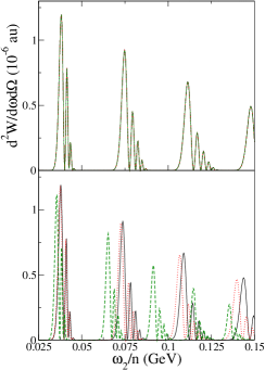
Figure 1: (Color online) Double differential spectrum $\frac{d^{2}W}{d\Omega_{2}d\omega{{}_{2}}}$ as a function of $\omega_{2}/n$, for incident frequencies $\,\omega_{1}=n\,\omega_{0}\,,\;\omega_{0}=1.17eV$; $n=1$ full (black) line, $n=2$ dotted (red) line, $n=10$ dashed (green) line. Upper plot: classical calculation, lower plot: quantum calculation.

Next we shall consider angular distributions $\,\frac{dW}{d\Omega_{2}}\,$ of the emitted photon. In Fig. 2 the angular distribution as a function of the angle $\,\theta_{\gamma-e}\,$ is represented for three values of the electron initial energy: (a) $\gamma=10^{3}$, corresponding to the initial electron energy $E_{1}\sim 511$ MeV, (b) $\gamma=10^{4}$ ( $E_{1}\sim 5.1$ GeV) and (c) $\gamma=10^{5}$ ($E_{1}\sim 51$ GeV), and for the values 0.5, 1 and 2 of the parameter $\eta$, marked on each graph.

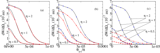
Figure 2: (Color Online) The angular distribution $\,\frac{dW}{d\Omega_{2}}\,$ for $\eta$=0.5, 1 and 2 (values marked on each graph) and $\gamma=10^{3}$ (a), $\gamma=10^{4}$ (b), $\gamma=10^{5}$ (c). Black lines: classical results (26), blue squares: numerical integration of (35), red circles: quantum results (14).

Values calculated in the framework of the classical theory (Thomson), using the analytical formula (26), are represented with black lines. The blue squares represent the values obtained by numerical integration over the emitted frequency of our formula (35); the agreement between the two is also a check of the accuracy of our classical code. The quantum (Compton) results, obtained by numerical integration of the double differential spectrum (14) are represented with red circles, which have been connected by lines in order to guide the eye. For $\,\gamma=10^{3}$ the classical and quantum results are practically identical; differences are found at $\,\gamma=10^{4}$ and they become large at $\gamma=10^{5}$. In all cases, the classical and quantum results have similar shapes; the quantum results are always lower than the corresponding classical ones which is a consequence of the fact that in the quantum case the spectrum is compressed toward lower frequencies (see also the discussion further on). When the field intensity increases, the angular distribution becomes “wider”, i.e. it spreads up to larger angles $\theta_{\gamma-e}$. In the monochromatic case, the angular distribution was analyzed by Goreslavskii et al. GRSL . For $\,\gamma\gg\eta\gg 1$, they have evaluated the opening angle of the cone in which the radiation is emitted, as inversely proportional to the factor $\gamma_{*}$ associated with the “dressed” electron momentum. For the geometry chosen here, $\gamma_{*}$ decreases with increasing $\,\eta$. We also note that the opening angle of the cone in which the radiation is emitted decreases with the increase of $\gamma$ at fixed $\,\eta\,$, in agreement also with the predictions made in GRSL .

In the following, in Figs. 3-6, we study in more detail the distribution of the emitted photons, by presenting the double differential spectra $\frac{d^{2}W}{d\Omega_{2}d\omega_{2}}$ as a function of the emitted frequency $\omega_{2}$, for a fixed value of $\,\theta_{\gamma-e}\,$. The calculations are made for the same initial scattering geometry (head-on collision) as in Fig. 2 and for the values $10^{4}$ and $10^{5}$ of the parameter $\,\gamma$.

In Fig. 3 we consider $\,\eta=0.5$ and $\gamma=10^{4}$; the three plots correspond, respectively, to $\,\theta_{\gamma-e}=0$ (a), $\,\theta_{\gamma-e}=5\times 10^{-5}\pi$ (b) and $\,\theta_{\gamma-e}=10^{-4}\pi$ (c). Classical results are drawn in full (black) lines, and the quantum ones in dashed (red) lines. The vertical thin lines indicate the positions of the discrete frequencies $\omega_{2}^{(N)}(I_{max})$, [Eq. (47) for Compton and (51) for Thomson]; in case (a) the values of $\,\omega_{2}^{(1)}(I=0)\,$ are also shown, marked with dashed lines. For the laser pulse, each line is replaced by a continuous distribution with the absolute maximum near the corresponding frequency $\omega_{2}^{(N)}(I_{max})$. If $\,\eta\,$ is not too large these distributions do not overlap.

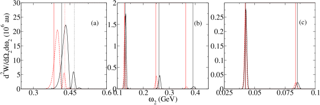
Figure 3: (Color online)Double differential spectrum $\frac{d^{2}W}{d\Omega_{2}d\omega_{2}}$ for $\gamma=10^{4}$ and $\eta=0.5$. $\theta_{\gamma-e}=0$ (a), $5\times 10^{-5}\pi$ (b) and $10^{-4}\pi$ (c). Full (black) line: classical calculation, dashed (red) line: quantum calculation. Thin vertical lines: the position of $\omega_{2}^{(N)}(I_{\mathrm{max}})$; dashed vertical lines in (a): the positions of $\omega_{2}^{(N)}(I=0)$.

We shall discuss first case (a), the backward emission, because in the context we consider (head-on collision, circularly polarized laser) the situation differs drastically from that at $\,\theta_{\gamma-e}\not=0\,$. In case (a) there is only one spectral region in the spectrum, a particularity that has a correspondence in the monochromatic limit, where only one line ($N=1$) appears, as explained in Sect. IV. The width of this maximum can be estimated, according to the previous section as $\omega_{2}^{(1)}(I=0)-\omega_{2}^{(1)}(I_{\mathrm{max}})$; the agreement between this estimation and the numerical results is seen on the graph.

At scattering angles $\,\theta_{\gamma-e}\not=0\,$, both Thomson and Compton spectra consist of a series of successive maxima located near the corresponding monochromatic positions [different values of $N$ in (50) and (46)] and with a small structure around the principal maximum. Due to the relatively low value of the parameter $\,\eta$, only a few maxima are present in the cases (b) and (c) of Fig. 3, and the first one is dominant. We notice that the new spectral regions appear as soon as $\,\theta_{\gamma-e}\,$ departs from 0, so they could influence the experimental observation of backward scattering at high intensity.

More maxima appear, except for the case (a), for a higher field intensity than in Fig. 3, as shown in Fig. 4, corresponding to $\,\eta=2$;

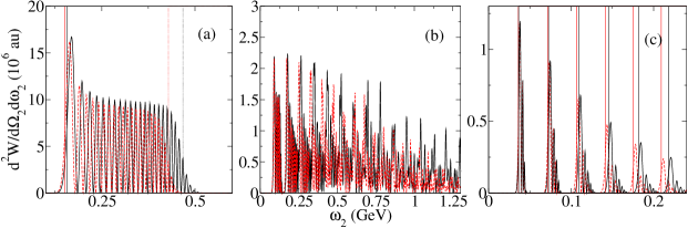
Figure 4: Same as 3 but $\eta=2$

also their structure becomes wider. The spectral region covered at $\theta_{\gamma-e}=0$ becomes very wide; as in Fig. 3, its width can be explained by the variable intensity during the pulse. For $\theta_{\gamma-e}=5\times 10^{-5}\pi\,$ the width of the successive maxima is so large that they practically overlap.

For increased electron energy ($\gamma=10^{5}$) more important differences between the classical and quantum results appear, in agreement with the observations made for the angular distribution $\frac{dW}{d\Omega_{2}}$, in connection with Fig. 2. Figures 5 and 6 correspond to the same values for $\eta\,$ as Fig. 3 and, respectively, Fig. 4, but $\gamma$ is $10^{5}$ and the angle $\,\theta_{\gamma-e}\,$ ten times smaller. The qualitative behaviour of the results is the same, nevertheless, on the one hand the shift of the quantum results with respect to the classical ones is much larger and on the other hand, the classical spectrum spreads to much larger frequencies than the quantum one, which explains the smaller value of the frequency integrated spectrum ($\,dW/d\Omega_{2}$, Fig. 2) for Compton than for Thomson scattering.

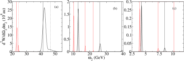
Figure 5: (Color online) Double differential spectrum $\frac{d^{2}W}{d\Omega_{2}d\omega_{2}}$ for $\gamma=10^{5}$ and $\eta=0.5$. $\theta_{\gamma-e}=0$ (a), $5\times 10^{-6}\pi$ (b) and $10^{-5}\pi$ (c). Dotted (red) line: classical calculation, full (black) line: quantum calculation. Thin vertical lines mark the position of $\omega_{2}^{(N)}(I_{\mathrm{max}})$; dashed vertical lines in (a) mark the positions of $\omega_{2}^{(N)}(I=0)$

Figure 6: Same as 5 but $\eta=2$

For the larger intensity $\eta=2$ in Fig. 6, the position of the maxima is very different in classical and quantum cases, as it is for the line positions in the monochromatic case, and the width of the peaks becomes very wide; the lower and upper limits for frequencies are close to the values for the maximum and zero intensity in the monochromatic case, marked with vertical lines on the graph (a) only. With increasing $\,\theta_{\gamma-e}\,$ the spectral region covered by radiation emission becomes narrower and it moves toward lower frequencies.

As we have just mentioned, the most important differences between classical and quantum predictions, are visible in Fig. 6. Although at first sight, the case (a) seems similar to the other cases, it is not so. As already explained, all that is seen in case (a) corresponds to a line in the monochromatic case, that with $\,N=1\,$, in both Thomson and Compton scattering. An increase of $\eta\,$ will result in a broadening of the spectrum toward low frequencies, as according to (46) $\omega_{2}\,$ decreases with the intensity. In the case (b) both in Compton and Thomson case many overlapping maxima are present; also the Compton results indicate an upper limit of the frequency for the whole spectrum, corresponding in the monochromatic case to the cut-off frequency (49), independent on intensity. For $\,\gamma=10^{5}$ this limit is $\omega_{\mathrm{cut-off}}\sim 51$ GeV, in both cases, as the two angles are very close. This value is practically equal to the kinetic energy of the incident electron. A further increase of the intensity will lead only to an increase of the intensity of this portion of the emitted spectrum, but will not extend it to larger frequencies. The value of the limit frequency can be changed only through the incident electron momentum magnitude and direction. For $\theta_{\gamma-e}=5\times 10^{-6}$ the classical spectrum spreads up to $\omega_{2}\sim 150$ GeV, while for $\theta_{\gamma-e}=5\times 10^{-6}$ the limit is $\omega_{2}\sim 250$ GeV. This limit is due only to the finite value of the parameter $\eta$; Were $\,\eta\,$ larger, additional maxima, located at larger values of $\omega_{2}$ would appear, as there is no limit to the frequency spectrum in Thomson scattering. One can conclude that in the studied conditions, the classical results cease to be valid.

Finally, we present an example of polarization analysis of the emitted spectrum for Thomson scattering. We now choose a geometry different from that used in the previous cases, with the incident electron momentum along the $\,Ox$ axis and orthogonal to the direction of propagation of the laser (always the $\,Oz$ axis). We have chosen $\,\gamma=10^{3}$, $\,\eta=1$ and the same frequency $\,\omega_{1}\,$, i.e. $\,\hbar\omega_{1}=1.17$ eV, as in the previous cases. The emitted photon is detected in the plane defined by the direction of propagation of the laser and the direction of the incident electron, at an angle $\theta_{e-\gamma}=2.5\times 10^{-4}\pi$ with respect to ${\bf p}_{1}$. In Fig. 7 are presented the spectral distributions of the two components of the emitted radiations $\,d^{2}W_{\sigma}^{\mathrm{cl}}/d\omega_{2}d\Omega_{2}$ (dashed green line) and $\,d^{2}W_{\pi}^{\mathrm{cl}}/d\omega_{2}d\Omega_{2}$ (full blue line) defined as in Eqs. (43) and (III), respectively. The results change in a visible manner with the laser polarization. In the case (a), when the laser is polarized along the electron initial direction, which corresponds to the choice $\,\zeta=0$ in Eq. (53), only the $\,\pi\,$ component is present in the spectrum. If the laser is circularly polarized [$\zeta=\pi/2$, case (b)], both components are present, the $\sigma$ component being favored. Finally, the graph (c) is for the laser field linearly polarized on the direction orthogonal to the initial electron direction ( $\zeta=\pi$), the geometry studied by Krafft et al. Krf2 . In this case the polarization of the successive peaks alternates: those with odd order have the $\,\pi$ polarization, while the even order peaks are $\,\sigma$ polarized.

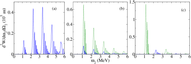
Figure 7: (Color online) $d^{2}W_{\sigma}^{\mathrm{cl}}/d\omega_{2}d\Omega_{2}$ [dashed (green) line] and $d^{2}W_{\pi}^{\mathrm{cl}}/d\omega_{2}d\Omega_{2}$ [full (blue) line] for $\gamma=10^{3}\,,$ $\eta=1$ and different laser polarizations: $\zeta=0$ (a), $\zeta=\pi/2$ (b), $\zeta=\pi\,$ (c) in Eq. (53).

VI Conclusions

We have considered the basic equations of Compton and Thomson scattering of a non-monochromatic electromagnetic plane wave on free electrons. We have derived the classical limit (35) of the quantum expression of the emitted radiation spectral and angular distribution (14), valid for any polarization of the laser, for unpolarized initial electrons and summed over scattered electron spin and emitted photon polarization. In Appendix B, we have reobtained the expression (35) by transforming the standard more general formula of classical electrodynamics (20). This latter calculation also allows the derivation of the contribution to the total distribution of the radiation with fixed polarization to be achieved. Analytic expressions for two particular polarization contributions are given in (43) and (III). These results are of the same type as those obtained by Krafft et al. Krf2 with a different analytical procedure and valid only for a linearly polarized pulse orthogonal to the initial electron direction. The differences between quantum and classical spectra, qualitatively discussed in Sect. IV, are illustrated by several graphs in Sect. V for the case of a circularly polarized pulse, head-on collisions and very energetic incident electrons. For electron energies above 500 MeV quantitative differences between classical and quantum results were shown. The influence of the laser polarization on the emitted radiation polarization is illustrated in Fig. 7, for the case of Thomson scattering.

Appendix A The electron trajectory

In a system of axis with the origin located at the initial position of the electron and the $Oz$ axis along the propagation direction of the laser pulse (the unity vector $\,{\bf n}_{1}\,$), the electron trajectory follows from the well-known equations F1

$$z(t) = \frac{c}{2(n_{1}\cdot p_{1})^{2}}\,\int_{\phi_{0}}^{\phi}d\chi\,\left\{[\,{\bf p}_{1\,\perp}-e{\bf A}(\chi)\,]^{2}+(mc)^{2}-(n_{1}\cdot p_{1})^{2}\,\right\}$$

$${\bf r}_{\perp}(t) = \frac{c}{n_{1}\cdot p_{1}}\,\int_{\phi_{0}}^{\phi}d\chi\,[\,{\bf p}_{1\,\perp}-e{\bf A}(\chi)\,]\,,\qquad\phi=t-\frac{z}{c}\,.$$ (54)

The first relation is an implicit equation from which one derives $\,z(t)\,$. Once this equation is solved, the position $\,{\bf r}_{\perp}\,$ in the plane orthogonal to the direction of propagation follows. As for $\,\phi=\phi_{0}\,$ one has $\,{\bf r}=0\,$, it follows that the value of $\,\phi_{0}\,$ coincides with the initial moment at which the electron is supposed to be free.

From (A) one obtains the velocity:

$$\bm{\beta}=\frac{{\bf v}}{c}=\,\frac{1}{c}\,\frac{d{\bf r}}{d\phi}\frac{d\phi}{dt}=\{\frac{{\bf p}_{1\perp}-e{\bf A}(\phi)}{n_{1}\cdot p_{1}}+\frac{[\,{\bf p}_{1\perp}-e{\bf A}(\chi)\,]^{2}-(n_{1}\cdot p_{1})^{2}+(mc)^{2}}{2(n_{1}\cdot p_{1})^{2}}\,{\bf n}_{1}\,\}\,\frac{d\phi}{dt}\\$$ (55)

with

$$\frac{d\phi}{dt}=\frac{2(n_{1}\cdot p_{1})^{2}}{[\,{\bf p}_{1\perp}-e{\bf A}(\chi)\,]^{2}+(n_{1}\cdot p_{1})^{2}+(mc)^{2}}\equiv F\,.\\$$ (56)

For $\,{\bf A}=0\,$ the velocity reduces to $\,c^{2}\,{\bf p}_{1}/E_{1}\,,$ with $\,E_{1}=c\sqrt{m^{2}c^{2}+{\bf p}_{1}^{2}}\,$. So, in the case of a laser pulse, the velocity at the end of the pulse is the same as the beginning of the pulse,

$$\bm{\beta}(t_{f})=\bm{\beta}(t_{\mathrm{in}})=c\frac{{\bf p}_{1}}{E_{1}}\,.$$ (57)

But, as is also known, the equations (A) allow the coordinates to be treated as depending explicitly on the variable $\,\phi\,$. These relations have been used in transforming the classical phase from (21) to (24).

Appendix B Transformation of Eq. (20)

We transform here the expression (20) of the classical spectrum. First, in order to avoid possible divergent integrals in the intermediate calculation, we define the integral $\,\tilde{\bf K}\,$ connected to the vector $\,{\bf K}\,$ by

$${\bf K}=\lim_{t_{1}\rightarrow-\infty\;t_{2}\rightarrow\infty}\left(\frac{e_{0}}{\pi\,\sqrt{8c}}\,\widetilde{\bf K}(t_{1},t_{2};\omega_{2},{\bf n}_{2})\right)\,,$$ (58)

where

$$\widetilde{\bf K}(t_{1},t_{2};\omega_{2},{\bf n}_{2})=\int_{t_{1}}^{t_{2}}\,\frac{dt}{\kappa^{2}}\,\exp[i\omega_{2}(t-\frac{{\bf n}_{2}\cdot{\bf r}(t)}{c})]\,{\bf n}_{2}\times[({\bf n}_{2}-\bm{\beta})\times\dot{\bm{\beta}}]\,.$$ (59)

We assume that the electromagnetic field is zero outside the interval $\,(t_{1},t_{2})\,$.

We perform several transformations.

1) The standard integration by parts Jks , based on

$$\frac{1}{\kappa^{2}}{\bf n}_{2}\times[({\bf n}_{2}-\bm{\beta})\times\dot{\bm{\beta}}]=\frac{d}{dt}\frac{{\bf n}_{2}\times({\bf n}_{2}\times\bm{\beta})}{\kappa}\,,$$

leads to the structure

$$\widetilde{\bf K} = {\bf n}_{2}\times({\bf n}_{2}\times{\bf L})\,,\qquad{\bf L}={\bf L}_{1}+{\bf L}_{2}\,$$ (60)

$${\bf L}_{1} = {\frac{\bm{\beta}}{\kappa}\,\exp[i\omega_{2}(t-\frac{{\bf n}_{2}\cdot{\bf r}(t)}{c})]\vline}_{\;t_{1}}^{\;t_{2}}$$ (61)

$${\bf L}_{2} = -{i}\,\omega_{2}\int_{t_{1}}^{t_{2}}\,dt\,\bm{\beta}\,\exp[i\omega_{2}(t-\frac{{\bf n}_{2}\cdot{\bf r}(t)}{c})]\,\,.$$ (62)

Both vectors $\,{\bf L}_{1}\,$ and $\,{\bf L}_{2}\,$ are in fact not well defined if the integration limits $\,t_{1}\,$ and $\,t_{2}\,$ go to $\,-\infty\,$ and to $\,\infty\,$, respectively. Nevertheless, for the electron initially at rest, as the velocity will be zero at the end of pulse, too, one has $\,{\bf L}_{1}=0\,$ and one gets the formula (22).

2) In the term $\,{\bf L}_{2}\,$ we make the change from the variable $\,t\,$ to the variable $\,\phi=t-{\bf r}\cdot{\bf n}_{1}/c\,$. We use the expression of $\,d\phi/dt\,$ in (56) and we write the phase $\,\Phi^{\mathrm{cl}}(p_{1};\phi)\,$ as in (24). The integration limits become $\,\phi_{1}=t_{1}-z(t_{1})/c\,$ and $\,\phi_{2}=t_{2}-z(t_{2})/c\,$.

3) Using (55), we write the expression of $\,\bm{\beta}\,$ as

$$\bm{\beta}=F\left(\frac{{\bf p}_{1\perp}-e{\bf A}}{n_{1}\cdot p_{1}}+\frac{1-F}{F}\,{\bf n}_{1}\right)\,,$$

then we split $\,\bm{\beta}\,$ as

$$\frac{\bm{\beta}}{F}=\frac{{\bf p}_{1}}{n_{1}\cdot p_{1}}+\frac{\widetilde{\bm{\beta}}}{F}\,,\qquad\frac{\widetilde{\bm{\beta}}}{F}=-\frac{e{\bf A}}{n_{1}\cdot p_{1}}+\left(-2\,e{\bf A}\cdot{\bf p}_{1}+e^{2}{\bf A}^{2}\right)\,\frac{{\bf n}_{1}}{2(n_{1}\cdot p_{1})^{2}}\,,$$ (63)

isolating the term that does not vanish in the absence of the electromagnetic field. Accordingly to this, we also split the integral $\,{\bf L}_{2}\,$ as

$${\bf L}_{2}={\bf L}_{2a}+{\bf L}_{2b}\,$$

with

$${\bf L}_{2a}=-i\,\omega_{2}\,\frac{{\bf p}_{1}}{n_{1}\cdot p_{1}}\,\int_{\phi_{1}}^{\phi_{2}}d\phi\,\exp[-i\Phi^{\mathrm{cl}}(p_{1};\phi)]\,,\qquad{\bf L}_{2b}=-i\,\omega_{2}\,\int_{\phi_{1}}^{\phi_{2}}\,d\phi\,\frac{\widetilde{\bm{\beta}}}{F}\,\exp[-i\Phi^{\mathrm{cl}}(p_{1};\phi)]\,.$$ (64)

4) We perform an integration by parts in $\,{\bf L}_{2a}\,$ based on

$$\exp\left(i\omega_{2}\phi\frac{n_{2}\cdot p_{1}}{n_{1}\cdot p_{1}}\right)=-\frac{i}{\omega_{2}}\,\frac{n_{1}\cdot p_{1}}{n_{2}\cdot p_{1}}\,\frac{d}{d\phi}\exp\left(i\omega_{2}\phi\frac{n_{2}\cdot p_{1}}{n_{1}\cdot p_{1}}\right)\,,$$

leading to

$${\bf L}_{2a}={\bf L}_{2a}^{(1)}+{\bf L}_{2a}^{(2)}\,,$$

with

$${\bf L}_{2a}^{(1)}=-{\frac{{\bf p}_{1}}{n_{2}\cdot p_{1}}\,\,\exp[-i\,\Phi^{\mathrm{cl}}(p_{1};\phi)]\vline}_{\;\phi_{1}}^{\;\phi_{2}}$$

and

$${\bf L}_{2a}^{(2)}=i\,\frac{\omega_{2}\,{\bf p}_{1}}{2n_{1}\cdot p_{1}}\,\int_{\phi_{1}}^{\phi_{2}}d\phi\,\,[\,\frac{n_{1}\cdot n_{2}}{2(n_{1}\cdot p_{1})^{2}}\,e^{2}{\bf A}^{2}+e{\bf W}\cdot{\bf A}\,]\,\exp[-i\,\Phi^{\mathrm{cl}}(p_{1};\phi)]\,,$$ (65)

with $\,{\bf W}\,$ defined in (25).

5) One notices easily that $\quad{\bf L}_{1}+{\bf L}_{2a}^{(1)}=0\,$ , as the velocity of the electron is the same at the beginning and at the end of the pulse [see (57)]. So the vector $\,\bf L\,$ in (59) we are looking for is expressed as

$$\widetilde{\bf K}(t_{1},t_{2};\omega_{2},{\bf n}_{2})={\bf n}_{2}\times[{\bf n}_{2}\times({\bf L}_{2a}^{(2)}+{\bf L}_{2b})]\,,$$ (66)

where $\,{\bf L}_{2a}^{(2)}\,$ and $\,{\bf L}_{2b}\,$ given by (65) and (64), respectively.

In the expression we have derived for $\,\widetilde{\bf K}(t_{1},t_{2};\omega_{2},{\bf n}_{2})\,$ we can take now the limits $\,\phi_{1}\rightarrow-\infty\,$ and $\,\phi_{2}\rightarrow\infty\,$, corresponding to $\,t_{1}\rightarrow-\infty\,$ and $\,t_{2}\rightarrow\infty\,$. By the transformations performed we have justified the final result, Eqs. (37) and (III), for the vector $\,{\bf K}\,$ in (20), valid for an electromagnetic plane wave.

References

- (1) J. H. Eberly, Progress in Optics, edited by E. Wolf, North Holland, Amsterdam 1969.
- (2) C. Bula et al., Phys. Rev. Lett 76, 3116 (1996); C. Bamber et al., Phys. Rev. D 60, 092004 (1999).
- (3) Y. I. Salamin, S. X. Hu, K. Z. Hatsagortsyan and C. H. Keitel, Physics Reports 427, 41 (2006).
- (4) F. Ehlotzky, K. Krajewska and J. Z. Kaminski, Rep. Prog. Phys. 72, 046401 (2009).
- (5) E. Esarey, S. K. Ride, Ph. Sprangle, Phys. Rev. E 48, 3003 (1993).
- (6) K. Lee, Y. H. Cha, M. S. Shin, B. H. Kim, and D. Kim, Phys. Rev. E 67, 026502 (2003).
- (7) P.F. Lan, P.X. Lu, W. Cao, and X.L. Wang, Phys. Rev. E 72, 066501 (2005).
- (8) M. Babzien et al., Phys. Rev. Lett. 96, 054802 (2006).
- (9) C. I. Moore, J. P. Knauer, and D. D. Meyerhofer, Phys. Rev. Lett. 74, 2439 (1995).
- (10) J. D. Jackson, Classical Electrodynamics, third edition, Wiley, 1998.
- (11) G. A. Krafft, Phys. Rev. Lett. 92, 204802 (2004).
- (12) G. A. Krafft, A. Doyuran and J. B. Rosenzweig, Phys. Rev. E 72, 056502 (2005).
- (13) F. V. Hartemann, J. R. Van Meter, A. L. Troha, E. C. Landahl, N. C. Luhmann, H. A. Baldis, A. Gupta, A. K. Kerman, Phys. Rev. E 58, 5001 (1998).
- (14) K. Lee and Y. H. Cha, M. S. Shin, B. H. Kim, and D. Kim, Optics Express 11, 309 (2003).
- (15) J. Gao, J. Phys. B: At. Mol. Opt. Phys. 39, 1345 (2006).
- (16) P.F. Lan, P.X. Lu, W. Cao, and X.L. Wang, J.Phys. B: At. Mol. Opt. Phys. 40, 403 (2007).
- (17) T. Heinzl, D. Seipt, and B. K¨ampfer, Phys. Rev. A 81, 022125 (2010).
- (18) F. V. Hartemann, H. A. Baldis, A. K. Kerman, A. Le Foll, N. C. Luhmann, Jr., and B. Rupp, Phys. Rev. E 64, 016501 (2001).
- (19) F. V. Hartemann, D. J. Gibson and A. K. Kerman, Phys. Rev. E 72, 026502 (2005).
- (20) C. Harvey, T. Heinzl and A. Ilderton, Phys. Rev. A 79, 063407 (2009).
- (21) T. Heinzl and A. Ilderton, Eur. Phys. J. D. 55, 359 (2009).
- (22) N. B. Narozhnyi and M. S. Fofanov, JETP 83, 14 (1996).
- (23) M. Boca and V. Florescu, Phys. Rev. A 80, 053403 (2009); M. Boca and V. Florescu, Phys. Rev. A 81, 039901(E) (2010).
- (24) P. Krekora, R. E. Wagner, Q. Su, and R. Grobe, Laser Phys. 12, 455 (2002).
- (25) J. Peatross, C. Mu¨ller, K. Z. Hatsagortsyan, and C. H. Keitel, Phys. Rev. Lett. 100, 153601 (2008).
- (26) H. A. Kramers, Phil. Mag. 46, 836 (1923).
- (27) L. Kim and R. H. Pratt, Phys. Rev. A 36, 45 (1987).
- (28) S. P. Goreslavski, S. V. Popruzhenko and O. V. Shcherbachev, Laser Phys. 9, 1039 (1999).
- (29) V. Hartemann, Nucl. Instr. and Methods in Physics Research, A 608, S1 (2009).
- (30) T. Heinzl, Journal of Physics: Conference Series 198, 012005 (2009).
- (31) I. V. Sokolov, J. A. Nees, V. P. Yanovsky, N. M. Naumova and G. A. Mourou, Phys. Rev. E 81, 036412 (2010).
- (32) L. S. Brown and T. W. B. Kibble, Phys. Rev. 133, A705 (1964).
- (33) E. S. Sarachik and G. T. Schappert, Phys. Rev. D 1, 2738 (1970).
- (34) D. Yu. Ivanov, G. L. Kotkin and V. G. Serbo, Eur. Phys. J. C 36, 127 (2004).
- (35) V. A. Lyulka, Zh. Eksp. Teor. Fiz. 67, 1638 (1974) [Sov. Phys. JETP 40, 815 (1975)].
- (36) Y. I. Salamin and F. H. M. Faisal, Phys. Rev. A 54, 4383 (1996); ibidem Phys. Rev. A 55, 3964 (1997).
- (37) Y. I. Salamin and F. H. M. Faisal, J. Phys. A: Math. Gen. 31, 1319 (1998).