Stability of nodal structures in graph eigenfunctions and its relation to the nodal domain count

Abstract.

The nodal domains of eigenvectors of the discrete Schrödinger operator on simple, finite and connected graphs are considered. Courant’s well known nodal domain theorem applies in the present case, and sets an upper bound to the number of nodal domains of eigenvectors: Arranging the spectrum as a non decreasing sequence, and denoting by $\nu_{n}$ the number of nodal domains of the $n$’th eigenvector, Courant’s theorem guarantees that the nodal deficiency $n-\nu_{n}$ is non negative. (The above applies for generic eigenvectors. Special care should be exercised for eigenvectors with vanishing components.) The main result of the present work is that the nodal deficiency for generic eigenvectors equals to a Morse index of an energy functional whose value at its relevant critical points coincides with the eigenvalue. The association of the nodal deficiency to the stability of an energy functional at its critical points was recently discussed in the context of quantum graphs [1] and Dirichlet Laplacian in bounded domains in $\mathbb{R}^{d}$ [6]. The present work adapts this result to the discrete case. The definition of the energy functional in the discrete case requires a special setting, substantially different from the one used in [1, 6] and it is presented here in detail.

1. Introduction

Courant’s nodal domain theorem can be viewed as a generalization of Sturm’s oscillation theorem to Laplace-Beltrami operators in higher dimensions. In the one-dimensional case, after ordering the spectrum of the Sturm-Liouville operator as an increasing sequence, the oscillation theorem guarantees that the $n$’th eigenfunction $f^{(n)}$ flips sign $\phi_{n}=n-1$ times in the open interval. Equivalently, the number of nodal domains $\nu_{n}$ — defined as the number of intervals where $f^{(n)}$ is of constant sign — equals $n$. The Sturm oscillation theorem can be written concisely as

(1) $$n=\nu_{n}=\phi_{n}+1\,.$$

In higher dimensions, the two equalities in (1) have to be modified. For $d>1$ there is no natural analogue of $\phi_{n}$, and therefore the right equality has to be discarded. Courant [10] showed that the left equality cannot hold in general, and it should be replaced by a bound:

(2) $$n\geq\nu_{n},$$

where $\nu_{n}$ is the number of maximal connected components of the domain on which the $n$’th eigenfunction has constant sign. Later studies [21, 22] have shown that equality holds only for finitely many eigenvectors. These states are referred to as Courant sharp.

Courant’s nodal domain theorem was extended to the Laplace operator on metric (quantum) graphs [13] and on discrete graphs [11] (see also references therein). The latter are the subject of the present work, and they will be discussed in detail in the next section.

The interest in counting the nodal domains increased in the mathematical and physical communities when it was realized that the nodal sequence $\{\nu_{n}\}_{n=1}^{\infty}$ stores metric information about the manifold where the Laplace-Beltrami operator is defined [7, 8, 9, 2, 19, 17]. It was shown, in particular, that in some cases the nodal sequences of isospectral domains are different [14, 17, 4, 3] and that in some other examples one can uniquely reconstruct the domain geometry from the given nodal sequence [18].

A new point of view was introduced in the pioneering article of Helffer, Hoffmann-Ostenhof and Terracini [15], where a variational approach was used to locate the Courant sharp eigenfunctions in the spectrum. Helffer et. al. investigated the Dirichlet Laplacian in a bounded domain $\Omega\in\mathbb{R}^{d}$ with $d\geq 2$. Partitioning $\Omega$ arbitrarily into $\nu$ sub-domains $\Omega_{k}$, they studied the lowest Dirichlet eigenvalue $\lambda_{1}(\Omega_{k})$ for each of the sub-domains. The maximal value amongst the $\lambda_{1}(\Omega_{k})$ for a given partition $\mathcal{P}$ (denoted as $\Lambda(\nu;\mathcal{P})$) can be viewed as the “energy” of the partition. Helffer et. al. proved that the partitions that minimize $\Lambda(\nu;\mathcal{P})$ coincide with the nodal partition induced by a Courant sharp eigenfunction if and only if the minimizing partition is bipartite.

We note that that the restriction of an eigenfunction $f^{(n)}$ to a nodal domain $\Omega_{k}$ is the ground state of the Dirichlet Laplacian on $\Omega_{n}$. The corresponding ground energy $\lambda_{1}(\Omega_{k})$ is equal to the eigenvalue $\lambda_{n}(\Omega)$ on the entire domain. Thus a partition corresponding to an eigenfunction will have a special property: $\lambda_{1}(\Omega_{k})$ is the same for all $k$. A partition with this property will be called an equipartition.

In two recent papers [1, 6] the approach of Helffer et. al. was broadened in a substantial way. It was shown that the functional $\Lambda(\nu;\mathcal{P})$, when restricted to a submanifold of equipartitions, becomes smooth. One can then study the critical points of $\Lambda(\nu;\mathcal{P})$, i.e. the points where the variation with respect to perturbations of the partition boundaries vanishes. It was shown that the critical $\nu$-partitions that are bipartite are in one-to-one correspondence with the nodal partitions of eigenfunctions with $\nu$ nodal domains. Moreover, the Morse index $\mu_{n}$ at the critical partitions equals the nodal deficiency of the corresponding eigenstate,

(3) $$\mu_{n}=n-\nu_{n}\ .$$

Thus, in the space of bipartite equipartitions, the critical points in the landscape of $\Lambda(\nu;\mathcal{P})$ are at eigenfunctions, and their stability (number of directions at which the critical point is a maximum) determines the nodal deficiency. The result (3) was proved for the Laplacian on metric graphs (quantum graphs) in [1] and was then shown to hold on domains in $\mathbb{R}^{d}$ in [6]. The present work complements the above mentioned articles by showing that (3) applies also for the discrete Schrödinger operator on finite graphs.

The variational approach used in [1, 6] crucially depends on the ability to smoothly change the boundaries of the domains. There is no direct analogue of this for discrete graphs. In the present work we show how one can use local variation of the potential in place of the variation of the partition boundaries. This is the chief new element introduced in this article, and it enables us to arrive at the main result of the present work, namely equality (3) for generic eigenvectors of the graph Shrödinger operator. The proof is provided in theorem 4.3.

There is another special feature that distinguishes graphs (metric or discrete) from other manifolds: one can describe the nodal structures in terms of points where the wave function changes its sign (for discrete graphs these will correspond to changes of the sign of the vertex eigenvector across a connecting edge). This allows us to reinterpret the bound on the number of nodal domains as a generalization of Sturm theorem. Indeed, we show that the right equality in (1) is replaced by upper and lower bounds on $\phi_{n}$, given in equation (29), Theorem 3.4.

The paper is organized in the following way. The next section provides a few definitions and known facts from spectral graph theory which are necessary for the ensuing discussion. The construction of partitions and the analogue of boundary variations require some ground work which is carried out in the section 3. The main results will be formulated and proved in section 4.

2. Definitions and general background

In the present chapter we provide a few definitions and facts which set the stage for the subsequent discussion.

A graph $G=(\mathcal{V},\mathcal{E})$ consists of a set of vertices $\mathcal{V}=\mathcal{V}(G)$ and a set of connecting edges $\mathcal{G}=\mathcal{E}(G)$. We shall use: $V(G)=|\mathcal{V}(G)|$ and $E(G)=|\mathcal{E}(G)|$. An edge $e\in\mathcal{E}(G)$ connecting the vertices $i,j\in\mathcal{V}(G)$ will be also denoted by $e=(i,j)=(j,i)$. We will use the notation $i\sim j$ to indicate that the vertices $i$ and $j$ are connected (are neighbors). A graph is simple if no more than a single edge connects two vertices and no vertex is connected to itself; otherwise the graph is a multi-graph. A graph is said to be connected if there exists a path of connected vertices between any two vertices in $\mathcal{V}$. Unless otherwise specified, the graphs we consider here are finite, connected and simple.

The connectivity of a graph $G$ is summarized by the adjacency matrix $A(G)$.

(4) $$[A(G)]_{i,j}=\left\{\begin{array}[]{cc}1,&\text{if }i\sim j\\ 0,&\text{otherwise}.\end{array}\right.$$

The degree $d_{i}$ of the vertex $i$ is the number of its neighbors; it can be expressed via the adjacency matrix as

$$d_{i}=\sum_{j\sim i}1=\sum_{j}A(G)_{i,j}.$$

The (first) Betty number of a connected graph is defined as

(5) $$\beta(G)=E(G)-V(G)+1\ .$$

This is the number of independent cycles on the graph.

A subgraph $G^{\prime}\subseteq G$ is itself a graph, defined by a subset of the vertex set $\mathcal{V}(G^{\prime})\subseteq\mathcal{V}(G)$ and a subset of the edge set $\mathcal{E}(G^{\prime})\subseteq\mathcal{E}(G)$. A factor (or spanning graph) of $G$ is a subgraph, $G^{\prime}\subseteq G$, which shares with $G$ the vertex set, $\mathcal{V}(G^{\prime})=\mathcal{V}(G)$. By removing $\beta(G)$ edges one can generate a factor which is a tree (a spanning tree). There exist more than one spanning tree. In what follows we shall often construct a sequence of connected factors by starting with $G$ and removing edges one at a time, while keeping the resulting factor connected and ending with a spanning tree after $\beta(G)$ steps.

A class of factors which will play a prominent role here are $\nu$-partitions.

Definition 2.1.

A $\nu$-partition of the graph $G$, denoted by $\mathcal{P}$, is a factor consisting of $\nu$ disjoint subgraphs, $P_{k}$, such that for any two vertices $i$ and $j$ in the same connected component $P_{k}$, if $(i,j)\in\mathcal{E}(G)$ then they are also connected in $P_{k}$. In other words, only the edges running between components were removed from $G$ to form $\mathcal{P}$. We write $\mathcal{P}=\bigcup_{k=1}^{\nu}P_{k}$.

We associate to any partition $\mathcal{P}$ a multi-graph $\widetilde{G}(\mathcal{P})$ with $\nu$ vertices. The vertices of $\widetilde{G}(\mathcal{P})$ are in one-to-one correspondence with the disjoint subgraphs of $\mathcal{P}$, while the edges of $\widetilde{G}(\mathcal{P})$ correspond to the edges that were removed from $G$. A partition is bipartite if its graph $\widetilde{G}(\mathcal{P})$ is bipartite, or a tree if $\widetilde{G}(\mathcal{P})$ is a tree, etc. Note that if $\widetilde{G}(\mathcal{P})$ is a tree, each pair of nodal domains is connected by at most one edge. Edges of this kind are referred to as bridges in the graph theory literature.

2.1. The Schrödinger Operator

The discrete Schrödinger operator acts on the Hilbert space of real vectors $f\in R^{V(G)}$ where the components $f_{i}$ are enumerated by the vertex indices $i$. The Schrödinger operator is a sum of two operators - the Laplacian and an on-site potential. The Laplacian is usually defined as

(6) $$L(G)=-A(G)+D(G)$$

where $A(G)$ is the adjacency matrix of $G$ and $D(G)$ is a diagonal matrix with $[D(G)]_{ii}=d_{i}$.

The on-site potential, $Q(G)$ is a diagonal matrix $[Q(G)]_{ii}=q_{i}\in\mathbb{R}$. However, since both $D$ and $Q$ are diagonal matrices and we will not impose any restrictions on the choice of site potentials $q_{i}$, we can “absorb” the degree matrix in the potential and define the Schrödinger operator

(7) $$H(G)=-A(G)+Q(G).$$

This convention significantly simplifies the notation later. The action of the Schrödinger operator (which we will also call the Hamiltonian) on a vector $f$ is given by

(8) $$\big{[}H(G)f\big{]}_{i}=-\sum_{j\sim i}f_{j}+q_{i}f_{i}\ .$$

The spectrum of (7) is discrete and finite. We denote it as

$$\sigma(G)=\{\lambda_{n}(G)\}_{n=1}^{V(G)}\qquad\text{with}\qquad\lambda_{1}(G)<\lambda_{2}(G)\leq\ldots\leq\lambda_{n}(G).$$

The eigenvector corresponding to $\lambda_{n}(G)$ will be denoted as $f^{(n)}=\{f_{i}^{(n)}\}_{i=1}^{V(G)}$.

Remark 2.2.

The definitions above can be generalized by associating positive weights $m_{i,j}=m_{j,i}$ to the connected bonds in $G$. The weighted adjacency matrix is defined as $[M(G)]_{i,j}=[A(G)]_{i,j}m_{i,j}$ . The results derived in the present paper are valid for this generalized version of the Schrödinger operator. However to simplify the notation we shall present the results for the case of uniform unit weights.

2.2. Nodal Domains

Let $f:G\rightarrow\mathbb{R}^{V(G)},\,f=\{f_{i}\}_{i=1}^{V(G)}$ be an arbitrary real function on the graph $G$. We define a strong nodal domain as a maximally connected subgraph of $G$ such that on all of its vertices the components of $f$ have the same sign. Vertices where $f$ vanishes do not belong to a strong nodal domain. A weak positive (respectively negative) nodal domain is defined as a maximally connected subgraph $Y$ such that for all $i\in\mathcal{V}(Y)$, $f_{i}\geq 0\,($respectively $f_{i}\leq 0)$. In this case, a weak nodal domain must contain at least one vertex where $f$ is non-zero. We will seek to understand the number of nodal domains of $n$-th eigenfunction of the Schrödinger operator (7).

Definition 2.3.

We will call an eigenfunction non-degenerate if it corresponds to a simple eigenvalue and its values at vertices are non-zero.

In this paper only non-degenerate eigenfunctions $f$ will be considered. In such cases the strong and weak nodal domains are the same and we denote by $\nu(G;f)$ their number. Thus, any $f:G\rightarrow(\mathbb{R}\backslash 0)^{V(G)}$ induces a bipartite $\nu(G;f)$-partition of $G$ with components which are the nodal domains. The number of edges of $G$ which are deleted to generate the partition will be denoted by $\phi(G;f)$, it is the number of sign flips of $f$ that occur along edges of $G$. The number of independent cycles in $G$ where $f$ has a constant sign (i.e. cycles that are contained in a single nodal domain) will be denoted by $\ell(G;f)$. The following identity relates these quantities [2]:

(9) $$\nu(G;f)=\phi(G;f)-\beta(G)+\ell(G;f)+1\ .$$

We shall focus on partitions induced by eigenvectors $f^{(n)}$ of (7). Because of the special role played by this function, we shall use the abbreviations $\nu_{n}=\nu(G;f^{(n)}),\ \phi_{n}=\phi(G;f^{(n)})\ {\rm and}\ \ell_{n}=\ell(G;f^{(n)})$. Here, Courant’s theorem [11], and its extensions [5] state that the number of nodal domains is bounded by

(10) $$n-\beta(G)\leq\nu_{n}\leq n\ .$$

Note that the lower bound on the number of nodal domains is not optimal. For well connected graphs such as $d$-regular graphs, $\beta(G)=\frac{V(G)(d-2)}{2}+1$ and hence, for $d\geq 4$, we have $n-\beta(G)\leq 0$ for all $n\leq V(G)$. An improved lower bound will be derived below.

Following [1, 15], we define,

Definition 2.4.

An eigenvector of the Hamiltonian (7) is Courant sharp if $\nu_{n}=n$.

The eigenvectors for the discrete Hamiltonian on trees are all Courant sharp [12] (see also [5]). While it is a special case of (10) with $\beta(G)=0$, it is the first step in the proof of the lower bound in (10) for general $\beta$.

The chromatic number $\chi$ of a graph can be used to give a bound on the number of nodal domains [20] : $\nu\leq V-\chi+2$. Hence, the only graphs for which the highest eigenvector (with $n=V(G)$) can be Courant sharp, are bipartite graphs where $\chi=2$.

3. Edge manipulations and the parameter dependent Hamiltonian

The main result of this paper is stated in Theorem 4.3. Its formulation requires definitions, concepts and facts which are provided in the first half of this section. To gain some intuition to the more formal discussions, we start by making the following simple observation.

Let $f=f^{(n)}$ be an non-degenerate eigenvector of the Hamiltonian $H(G)$, see Definition 2.3. Let $G^{\prime}$ be a connected factor of $G$ obtained by deleting an edge $e=(i,j)$. Following [5], we will modify the potential at the vertices $i$ and $j$ in such a way that $f$ is an eigenfunction of the factor $G^{\prime}$ with an eigenvalue that equals $\lambda_{n}(G)$. That is, there is $m$, such that $\lambda_{m}(G^{\prime})=\lambda_{n}(G)$. Note that $n$ and $m$ are not necessarily equal, and the other eigenvalues and eigenfunctions of $H(G^{\prime})$ need not coincide with those of $H(G)$. To work out the necessary modification to the potentials we rewrite (7) at site $i$

$$(H(G)f)_{i}=-\sum_{k\sim i}f_{k}+q_{i}f_{i}=-\sum_{{k\sim i},\,{k\neq j}}f_{k}+\left(q_{i}-\frac{f_{j}}{f_{i}}\right)f_{i}$$

and similarly at site $j$,

$$(H(G)f)_{j}=-\sum_{k\sim j,\,k\neq i}f_{k}+\left(q_{j}-\frac{f_{i}}{f_{j}}\right)f_{j}\ .$$

Thus,

(11) $$H(G)f=\left(-A(G^{\prime})+\widetilde{Q}(G^{\prime})\right)f\ ,$$

where the potential $\widetilde{Q}(G^{\prime})$ coincides with the original potential $Q(G^{\prime})$ on all vertices except the vertices $i$ and $j$ where the potential is modified to be

(12) $$\tilde{q}_{i}=q_{i}-\frac{f_{j}}{f_{i}}\qquad\tilde{q}_{j}=q_{j}-\frac{f_{i}}{f_{j}}.$$

The operator which multiplies $f$ on the right hand side of (11) above is a Hamiltonian operator for the factor $G^{\prime}$,

(13) $$H(G^{\prime})=-A(G^{\prime})+\widetilde{Q}(G^{\prime})\ .$$

Clearly $f$ is an eigenvector of $H(G^{\prime})$ corresponding to an eigenvalue which equals $\lambda_{n}(G)$ but whose position $m$ in $\sigma(G^{\prime})$ is not necessarily $n$.

This formal exercise acquires more substance once the modified potentials are defined by replacing in (12) the quotient $\frac{f_{j}}{f_{i}}$ with a real non zero parameter $\alpha$ and $\frac{f_{i}}{f_{j}}$ with $1/\alpha$. The resulting parameter dependent Hamiltonian $H(G^{\prime};\alpha)$ for the factor $G^{\prime}$ is defined as

(14) $$H(G^{\prime};\alpha)=H(G)+B(\alpha).$$

where the perturbation $B=B(\alpha)$ has only four non-vanishing entries,

(15) $$B_{i,i} =-\alpha, B_{i,j} =1$$

(16) $$B_{j,i} =1 B_{j,j} =-1/\alpha$$

The matrix $B(ij)$ has rank $1$, with a single non vanishing eigenvalue $-\alpha-\frac{1}{\alpha}$.

The following theorem is due to Weyl (see, for example, [16]) and will be extensively used in the sequel.

Theorem 3.1.

Let $A,B,C$ be real and symmetric $N\times N$ matrices with $C=A+B$. Denote by $a_{1}\leq a_{2}\leq\cdots a_{N}$ and $c_{1}\leq c_{2}\leq\cdots c_{N}$ the spectra of $A$ and $C$ respectively. If $B$ is of rank $1$ then the spectra of $C$ and $A$ interlace in the following way:

(17) $$\cdots\leq a_{k-1}\leq c_{k-1}\leq a_{k}\leq c_{k}\leq\cdots\qquad\text{if }B\geq 0,$$

and

(18) $$\cdots\leq a_{k-1}\leq c_{k}\leq a_{k}\leq c_{k+1}\leq\cdots\qquad\text{if }B\leq 0,$$

After all these preparations we can arrive to the following theorem.

Theorem 3.2.

Let $G$ be a simple, connected graph with a Hamiltonian $H(G)$, and let $G^{\prime}$ be a connected factor obtained by deleting the edge $(i,j)$ with parametrized Hamiltonian $H(G^{\prime};\alpha)$ defined by (14)-(16). Let $\lambda_{m}(G^{\prime};\alpha)$ and $f^{(m)}(\alpha)$ be the $m$’th eigenvalue and the corresponding eigenvector of $H(G^{\prime};\alpha)$. Consider the the eigenvalue $\lambda_{m}(G^{\prime};\alpha)$ as a function of $\alpha$. Its critical points $\alpha^{+}$ and $\alpha^{-}$ satisfy the equation

(19) $$\alpha=\pm\frac{f_{j}^{(m)}(\alpha)}{f_{i}^{(m)}(\alpha)}$$

with the corresponding sign.

Furthermore, as long as $\alpha^{+}\neq 0$ and finite, $\lambda_{m}(G^{\prime};\alpha^{+})$ is an eigenvalue of $H(G)$ whose position in $\sigma(G)$ is $n\in\{m-1,m,m+1\}$. The eigenvector $f^{(m)}(\alpha^{+})$ is the corresponding eigenvector of $H(G)$.

Conversely, if $f^{(n)}$ is an non-degenerate eigenvector of $H(G)$ then

(20) $$\alpha^{+}=\frac{f^{(n)}_{j}}{f^{(n)}_{i}}$$

is a critical point of $\lambda_{m}(G^{\prime};\alpha)$ where $m$ is such that $n\in\{m-1,m,m+1\}$.

Proof.

If $f^{(m)}(\alpha)$ is normalized, by first order perturbation theory we have

(21) $$\frac{{\rm d}\lambda_{m}(G^{\prime},\alpha)}{{\rm d}\alpha}=\left(f^{(m)}(\alpha),\ \frac{{\rm d}H(G^{\prime};\alpha)}{{\rm d}\alpha}f^{(m)}(\alpha)\right)$$

The only $\alpha$ dependent entries of $H(G^{\prime};\alpha)$ are the off-diagonal terms in $B$, see (15)-(16). Hence

(22) $$\frac{{\rm d}\lambda_{m}(G^{\prime},\alpha)}{{\rm d}\alpha}=-\left(f^{(m)}_{i}(\alpha)\right)^{2}+\frac{1}{\alpha^{2}}\left(f^{(m)}_{j}(\alpha)\right)^{2}\ ,$$

which is equal to zero at the solutions of equation (19).

From now on, we consider only the relevant critical points $\alpha^{+}$. At $\alpha^{+}$ one can easily check that

$$B(\alpha^{+})f^{(m)}(\alpha^{+})=0$$

and therefore

$$\lambda_{m}(G^{\prime};\alpha^{+})f^{(m)}(\alpha^{+})=H(G^{\prime};\alpha^{+})f^{(m)}(\alpha^{+})=H(G)f^{(m)}(\alpha^{+}).$$

Conversely, if $f^{(n)}$ is an non-degenerate eigenvector of $H(G)$ then it was shown in equation (11) that $f^{(n)}$ is an eigenvector of $H(G^{\prime};\alpha)$ for $\alpha$ determined by equation (20).

Finally, the matrix $B$ is of rank-$1$ and Weyl’s theorem 3.1 guarantees that the spectra of $H(G)$ and $H(G^{\prime})$ interlace according to (17) or (18), showing that $n\in\{m-1,m,m+1\}$. ∎

Further insight can be gained by examining closely how the position of the eigenvalue in the spectrum and the number of nodal domains change depending on the sign and the type (minimum or maximum) of the critical point. Note that we will shift the point of view and will use $G^{\prime}$ as the base graph, i.e. we will investigate the change in the above quantities when an edge is added back.

Let $\alpha^{c}$ denote a relevant critical point of $\lambda_{m}(G^{\prime};\alpha)$. We start with the case $\alpha^{c}>0$. Weyl’s theorem (17) implies that for all $\alpha>0$ (that is $B\leq 0$),

$$\lambda_{m-1}(G)\leq\lambda_{m}(G^{\prime};\alpha)\leq\lambda_{m}(G).$$

At the critical point $\alpha=\alpha^{c}$ the value $\lambda_{m}(G^{\prime};\alpha^{c})$ belongs to the spectrum of $H(G)$ and therefore equals either $\lambda_{m-1}(G)$ or $\lambda_{m}(G)$. Hence, $\lambda_{m}(G^{\prime};\alpha^{c})$ is a maximal value of $\lambda_{m}(G^{\prime};\alpha)$ if it equals $\lambda_{m}(G)$ and a minimal value if it equals $\lambda_{m-1}(G)$. For future use it is convenient to introduce the following notation. Let $M(ij)$ take the value $+1$ if the critical point is a maximum, and $0$ if it is a minimum. Let $\Delta n(ij)$ stand for the shift in the position of the eigenvalue in the spectrum, from its position in $\sigma(G^{\prime},\alpha^{c})$ to its position in $\sigma(G)$. One can summarize the findings so far by the following statement:

(23) $${\rm For}\ \alpha^{c}>0\ \ :\ \ M(ij)-\Delta n(ij)=1.$$

Similarly, for $\alpha^{c}<0$, Weyl’s theorem (18) implies that

$$\lambda_{m}(G)\leq\lambda_{m}(G^{\prime};\alpha)\leq\lambda_{m+1}(G).$$

Hence, $\lambda_{m}(G^{\prime};\alpha^{c})$ must attain either the maximal value $\lambda_{m+1}(G)$ or the minimal value $\lambda_{m}(G)$. Using the same notation as above we find:

(24) $${\rm For}\ \alpha^{c}<0\ \ :\ \ M(ij)-\Delta n(ij)=0$$

More information on the transition from $G$ to $G^{\prime}$ is gained by viewing the eigenvector $f^{(m)}(\alpha^{c})$ first as an eigenvector on $G^{\prime}$ and then as an eigenvector on $G$. This dual view point is now applied to follow the variation in the number of cycles with constant sign and the number of nodal domains, as one counts them with respect to $G^{\prime}$ or to $G$. It is important to remember that the sign of $\alpha^{c}$ is the relative sign of the $i$ and $j$ components $f^{(m)}(\alpha^{c})$ across the edge $(i,j)$.

Starting with $\alpha^{c}<0$, the number of nodal domains and the number of loops of constant sign are not affected by the transition from $G^{\prime}$ to $G$ since $f_{j}/f_{i}<0$ implies that $i$ and $j$ are in nodal domains with different signs. Denoting by $\Delta\ell(ij)$ the change in the number of loops with constant sign, and by $\Delta\nu(ij)$ the change in the number of nodal domain, we have

(25) $${\rm For}\ \alpha^{c}<0\ \ :\ \ \Delta\ell(ij)-\Delta\nu(ij)=0\ .$$

On the other hand, for $\alpha^{c}>0$ either the number of nodal domains or the number of cycles of constant sign will change. Indeed, the edge $(i,j)$ either connects two vertices that already belong to the same nodal domain, increasing $\ell(f^{(m)})$ by $1$ (and leaving $\nu(f^{(m)})$ unchanged) or it connects two nodal domains of the same sign, in which case $\nu(f^{(m)})$ decreases by $1$ while $\ell(f^{(m)})$ remains constant. This leads to

(26) $${\rm For}\ \alpha^{c}>0\ \ :\ \ \Delta\ell(ij)-\Delta\nu(ij)=1\ .$$

Comparing (24) to (25) and (23) to (26), the observations above can summarized by:

(27) $$\Delta\ell(ij)-\Delta\nu(ij)=M(ij)-\Delta n(ij)\ ,$$

which is valid for both signs of $\alpha^{c}$.

The discussion so far centered on a factor $G^{\prime}$ which differs from the original graph $G$ by the deletion of a single edge. However, by successive applications of Theorem 3.2 it can be generalized to any connected factor of $G$ obtained by the elimination of an arbitrary number of edges while modifying the appropriate vertex potentials. The set of parameters will be denoted by $\alpha=\{\alpha_{e}:e\in\mathcal{E}(G)\setminus\mathcal{E}(G^{\prime})\}$, the parameter dependent Hamiltonian is $H(G^{\prime},\alpha)$, and $\lambda_{m}(G^{\prime};\alpha)$ is its $m$’th eigenvalue.

Corollary 3.3.

Let $G$ be a graph as previously and $G^{\prime}$ a connected factor obtained by deleting $k\leq\beta(G)$ edges from $G$. Let $\alpha^{c}$ be a relevant critical point of $\lambda_{m}(G^{\prime};\alpha)$. Then, provided that none of the components of $f^{(m)}(\alpha^{c})$ vanishes at vertices where edges were added, $\lambda_{m}(G^{\prime};\alpha^{c})=\lambda_{n}(G)\in\sigma(G)$ with $|n-m|\leq k$. The corresponding eigenvectors are the same.

The lower bound on the number of nodal domains, the left part of equation (10), was proved by chaining the operations of edge removal [5]. In fact, a more careful book-keeping allows us to sharpen the lower bound (see [1] for the same inequality in the context of quantum graphs).

Theorem 3.4.

Let $f^{(n)}$ be the $n$-th eigenfunction of the Hamiltonian $H(G)$ such that the corresponding eigenvalue is simple and $f^{(n)}$ has no zero components. Then the number of nodal domains of $G$ with respect to $f^{(n)}$ satisfies

(28) $$n-(\beta(G)-\ell_{n})\leq\nu_{n}\leq n.$$

Correspondingly, the number $\phi_{n}$ of edges across which the eigenvector $f^{(n)}$ changes its sign satisfies the bound

(29) $$n-1\leq\phi_{n}\leq n+(\beta(G)-\ell_{n})-1.$$

Remark 3.5.

Note that the lower bound on $\nu_{n}$, the quantity $n-(\beta(G)-\ell_{n})$ is always non-negative.

Remark 3.6.

Equation (29) is the generalization of Sturm’s oscillation theorem to discrete graphs.

Proof of Theorem 3.4.

We cut $\beta$ edges of the graph $G$, modifying the potential accordingly, until we arrive to a tree $T$, such that $f=f^{(n)}$ is it eigenfunction. It is eigenfunction number $m$ and, since it is a tree, Fiedler theorem [12] implies it has $\nu_{m}(T)=m$ nodal domains. Also, $\ell_{m}(T)=0$, because there are no cycles on a tree.

We rewrite equation (27) in the form

$$\Delta\nu(e)=\Delta n(e)+\Delta\ell(e)-M(e),$$

where $e$ is the removed edge. Adding back the removed edges one by one and adding the above identities to the equation $\nu_{m}(T)=m$ we arrive at

$$\nu_{n}(G)=n+\ell_{n}-\sum M(e).$$

Since the number of maxima in the sequence is at most $\beta$, the number of nodal domains $\nu_{n}(G)$ is at least $n+\ell_{n}-\beta$, proving inequality (28) (the upper bound is due to [11]). Substituting equation (9) for $\nu_{n}$, we obtain inequality (29). ∎

Corollary 3.7.

If $f^{(n)}$ satisfies the conditions of Theorem 3.4 and its nodal partition graph $\widetilde{G}$ is a tree (or, equivalently, the edges on which $f^{(n)}$ changes sign do not lie on cycles of the graph), then $f^{(n)}$ is Courant-sharp: $\nu_{n}=n$.

Proof.

Indeed, if $\widetilde{G}$ is a tree, then no cycles are broken when removing the edges connecting the nodal domains and $\ell_{n}=\beta$. ∎

4. Critical Partitions - the main theorems and proofs

So far we discussed the reduction of a graph to its connected factors. The generation of partitions (disconnected factors) requires the introduction of some more concepts and definitions. Let $\mathcal{P}$ be a bipartite $\nu(G)$-partition of $G$, see Definition 2.1 and the discussion below it. We denote by $\mathcal{E(P)}$ the edge set of $\mathcal{P}$. Since we wish to characterize the partitions that appear as nodal domains, we will ofter refer to the connected components $P_{k}$ of $\mathcal{P}$ as “domains”.

Let $\phi(G;{\mathcal{P}})$ denote the number of edges in $\mathcal{E}(G)\backslash\mathcal{E}(\mathcal{P})$. Construct the Hamiltonian $H(\mathcal{P};\alpha)$, $\alpha\in\mathbb{R}^{\phi(G)}$ where for each deleted edge $e=(i,j)$, $i<j$, the potentials $\alpha_{e}$ and $\alpha_{e}^{-1}$ are added to the vertices $i$ and $j$ as was explained above. Note that the ordering of the vertices in an edge can be chosen arbitrarily; we chose $i<j$ for definiteness. The Hamiltonian $H(\mathcal{P};\alpha)$ is block-diagonal, namely

$$H(\mathcal{P};\alpha)=\bigoplus_{k=1}^{\nu(G)}H(P_{k};\alpha).$$

Let $\lambda_{1}(P_{k};\alpha)$ be the lowest eigenvalue of $H(P_{k};\alpha)$ with the corresponding eigenvector denoted by $g(P_{k};\alpha)$. Note that since $g(P_{k};\alpha)$ is a ground state, all its components have the same sign. We extend $g(P_{k};\alpha)$ to all vertices of the graph $G$ by setting $g_{s}(P_{k};\alpha)=0$ for $s\not\in\mathcal{V}(P_{k})$. We assume $g(P_{k};\alpha)$ is normalized and non-negative,

(30) $$\sum_{s\in\mathcal{V}(P_{k})}\left|g_{s}(P_{k};\alpha)\right|^{2}=\sum_{s\in\mathcal{V}(G)}\left|g_{s}(P_{k};\alpha)\right|^{2}=1,\qquad g_{s}(P_{k};\alpha)\geq 0.$$

Definition 4.1.

Let $\mathcal{P}$ be a bipartite $\nu$-partition of $G$ with the parameter dependent Hamiltonian $H(\mathcal{P};\alpha)$. An equipartition is a pair $(\mathcal{P},\alpha^{\prime})$, where $\alpha^{\prime}\in\mathbb{R}^{\phi(G;{\mathcal{P}})}$ is a vector of parameters such that all the lowest eigenvalues $\lambda_{1}(P_{k};\alpha^{\prime})$ are equal,

(31) $$\lambda_{1}(P_{1};\alpha^{\prime})=\lambda_{1}(P_{2};\alpha^{\prime})=\cdots=\lambda_{1}(P_{\nu};\alpha^{\prime}).$$

Consider the set $\mathcal{Q}(\mathcal{P})\subset\mathbb{R}^{\phi(G;{\mathcal{P}})}$ in the space of parameters $\alpha$ where equation (31) is satisfied (equivalently, all $\alpha$ such that $(\mathcal{P},\alpha)$ is an equipartition). On this set, the function $\Lambda(\mathcal{P};\alpha^{\prime})=\lambda_{1}(P_{k};\alpha^{\prime})$ will be referred to as the equipartition energy. Obviously, the index $k$ is arbitrary.

Intuitively, the $(\nu-1)$ equalities in (31) reduce the number of independent variables required to define the equipartition energy from $\phi(G;{\mathcal{P}})$ to $\eta:=\phi(G;{\mathcal{P}})-(\nu-1)$. Notice that, because of (9),

(32) $$\eta=\phi(G;\mathcal{P})-(\nu-1)=\beta(G)-\ell(G;\mathcal{P})\geq 0\ .$$

If the partition $\mathcal{P}$ is induced by an eigenvector $f^{(n)}$ of $H(G)$ then it also generates an equipartition with the vector $\alpha^{c}$ of parameters defined by

(33) $$\alpha^{c}_{e}=\frac{f^{(n)}_{j}}{f^{(n)}_{i}},\qquad\text{for each }e=(i,j)\in\mathcal{E}(G)\setminus\mathcal{E}(\mathcal{P}),\quad i<j.$$

Then the equipartition energy coincides with the eigenvalue of $G$, $\Lambda(\mathcal{P};\alpha^{c})=\lambda_{n}(G)$. In the sequel we shall consider the equipartition energy in the neighborhoods of these special points. Note that in the definition above the vertices $i$ and $j$ belong to different nodal domains. Therefore the special values of the parameters $\alpha_{e}$ are negative. This is why from now on we restrict our attention to the negative subspace of the parameter space, $\mathbb{R}_{-}^{\phi(G,\mathcal{P})}$.

The main results of the paper can now be formulated in terms of two theorems which distinguish between the cases $\eta=0$ and $\eta>0$.

Theorem 4.2.

Let $\mathcal{P}$ be a bipartite $\nu$-partition of $G$ with $\eta=\phi(G;\mathcal{P})-(\nu-1)=0$. Then $\mathcal{P}$ is a tree partition and there exists at most one equipartition $(\mathcal{P},\gamma)$, such that $\gamma\in\mathbb{R}_{-}^{\phi(G;\mathcal{P})}$. The value $\lambda=\Lambda(\mathcal{P};\gamma)$ is the $\nu$-th eigenvalue in the spectrum of $G$, and the corresponding eigenvector is Courant sharp.

Proof.

By definition of the partition graph $\widetilde{G}(\mathcal{P})$, it has $\nu$ vertices and $\phi(G;\mathcal{P})$ edges. Therefore its Betti number is $\phi(G;\mathcal{P})-\nu+1=0$ and it is a tree (see an illustration in Fig. 1(b) ignoring the dashed edges).

Let $\gamma$ be a vector of negative parameters such that $(\mathcal{P},\gamma)$ is an equipartition. The functions $g(P_{k},\gamma)$, normalized as in (30), can be used to construct an eigenvector of $H(G)$. Consider

(34) $$f=\sum_{q=1}^{\nu_{n}}t_{k}\,g(P_{k};\gamma),$$

where the coefficients $t_{k}$ are determined as follows. Pick arbitrarily one of the domain in $\mathcal{P}$, say $P_{1}$, to be the “root” of the partition tree and let $t_{1}=1$. For every domain $P_{r}$ adjacent to $P_{1}$ on the partition tree, let $e=(i,j)$ be the unique edge connecting $P_{1}$ to $P_{r}$ with $i\in P_{1}$ and $j\in P_{r}$. Without loss of generality assume that $i<j$ and take

$$t_{r}=t_{1}\gamma_{e}\frac{g_{i}}{g_{j}}.$$

Continue the process recursively to domains at larger distances from $P_{1}$. The tree structure guarantees that this covers the entire set of domains on the graph without ever reaching a domain for which the variable $t$ has been previously computed. Note that the values of $t$ alternate in sign, leading to the function $f$ whose nodal partition is precisely $\mathcal{P}$. We will now show that the resulting function $f$, equation (34), is an eigenvector of $H(G)$.

Start with the Hamiltonian $H(\mathcal{P};\gamma)$ and observe that since $f$ is composed out of eigenvectors of the connected components of $H(\mathcal{P};\gamma)$ that share the same eigenvalue,

$$H(\mathcal{P};\gamma)f=\Lambda(\mathcal{P};\gamma)f.$$

We will now add the edges from $\mathcal{E}(G)\setminus\mathcal{E}(\mathcal{P})$ one by one. For simplicity of notation we will consider the addition of the edge $e=(i,j)$ between the components $P_{1}$ and $P_{r}$. The addition of the edge results in a matrix $B$ defined by (15)-(16) with $\alpha=\gamma_{e}$. The relevant elements of the vector $f$ are

$$f_{i}=t_{1}g_{1},\qquad f_{j}=t_{r}g_{j}=t_{1}\gamma_{e}g_{i}.$$

A direct computation shows that $Bf=0$ and therefore $f$ remains an eigenfunction of the modified graph with the same eigenvalues. Proceeding similarly with the other edges we conclude that $H(G)f=\Lambda(\mathcal{P};\gamma)f$.

The function $f$ has $\nu$ nodal domains with respect to the graph $G$. From Corollary 3.7 we get that the function $f$ as an eigenfunction of $H(G)$ is Courant-sharp, that is, its index is $\nu$. Finally, since there is at most one Courant-sharp eigenfunction with $\nu$ domains, the equipartition is unique. ∎

Let $f^{(n)}$ be a non-degenerate eigenvector corresponding to the eigenvalue $\lambda_{n}(G)$. If the corresponding partition $\mathcal{P}$ is not a tree, there will be other equipartitions locally around the special point (33). Namely, we shall consider a ball $\mathcal{B}_{\epsilon}(\alpha^{c})$ of radius $\epsilon$ centered at $\alpha^{c}$ defined by (33). The value of $\epsilon>0$ is chosen sufficiently small so that the following two conditions are satisfied: (i) the variation in the equipartition energy $\Lambda(\mathcal{P};\alpha)$ is smaller than the minimal separation between successive eigenvalues in $\sigma(G)$ and (ii) none of the hyper-planes $\alpha_{e}=0$ intersect the ball. The discussion which follows is restricted to $\alpha\in\mathcal{B}_{\epsilon}(\alpha^{c})$ and thus, only local properties of the equipartition energy function are considered.

Theorem 4.3.

Let $\mathcal{P}$ be a bipartite $\nu$ partition of $G$ with $\eta=\phi(G;\mathcal{P})-(\nu-1)>0$ and $H(\mathcal{P};\alpha)$ be the associated parameter dependent Hamiltonian. If there exists an equipartition $(\mathcal{P},\widetilde{\alpha})$, then, in the vicinity of $\widetilde{\alpha}$ the set $\mathcal{Q}(\mathcal{P})$ of equipartitions forms a smooth $\eta$-dimensional submanifold of $\mathbb{R}^{\phi(G)}$.

The point $\alpha^{c}\in\mathbb{R}_{-}^{\phi(G)}$ is a critical point of the equipartition energy $\Lambda(\mathcal{P};\alpha)$ on the manifold $\mathcal{Q}(\mathcal{P})$ if and only if it corresponds to an non-degenerate eigenfunction with eigenvalue $\Lambda(\mathcal{P};\alpha^{c})$ and nodal domains $\mathcal{P}$. Furthermore, if $\Lambda(\mathcal{P};\alpha^{c})$ is the $n$-th eigenvalue in the spectrum, the Morse index $\mu_{n}$ of the critical point $\alpha^{c}$ satisfies

(35) $$\mu_{n}\ =\ n-\nu_{n}.$$

Proof.

We start by describing a parametrization of the manifold of equipartitions by $\eta$ independent parameters $\{\xi_{k}\}_{q=1}^{\eta}$. The construction is local around an existing equipartition. Start with the partition $\mathcal{P}$ (see Fig. 1(a)), and remove $\eta=\phi-(\nu-1)$ edges which connect different nodal domains, leaving $\nu(G)-1$ bridge edges which turn the partition graph $\tilde{G}(\mathcal{P})$ into a tree (as in Fig. 1(b)). The set of removed edges will be denoted by $X(\mathcal{P})$. Every deletion of an edge $e=(i,j)$ is accompanied by the modification of the vertex potentials at the vertices $i$ and $j$ by a parameter $\xi_{e}$ as usual. This partial set of $\eta$ parameters $\xi_{e}$ uniquely defines the equipartition energy. Indeed, the graph which was produced by the deletion of edges and which we denote by $G_{\xi}$ is exactly of the kind which was discussed in theorem 4.2. Since we started at an existing equipartition $(\mathcal{P},\widetilde{\alpha})$, it corresponds to an equipartition $(\mathcal{P},\widetilde{\beta})$ of the graph $G_{\widetilde{\xi}}$. Here $\widetilde{\beta}$ is a set of $\nu(G)-1$ entries of $\widetilde{\alpha}$ that correspond to edges $e\not\in X(\mathcal{P})$. The $\eta$ parameters $\widetilde{\xi}$, on the other hand, are the entries of $\widetilde{\alpha}$ that correspond to the edges $e\in X(\mathcal{P})$.

From Theorem 4.2 we conclude that the equipartition corresponds to a Courant-sharp eigenfunction $\psi^{(\nu)}(G_{\widetilde{\xi}})$. Under local variation of the parameters $\xi$ the eigenfunction $\psi^{(\nu)}(G_{\xi})$ remains Courant-sharp and induces an equipartition of the graph $G_{\xi}$ and, therefore, of the graph $G$. Moreover, the eigenfunction is smooth as a function of the parameters $\xi$. This allows us to define the parameters $\alpha$ (thus constructing a locally smooth immersion $\mathcal{Q}(\mathcal{P})\to\mathbb{R}^{\phi(G)}$ ) in the following manner. There is one parameter for each edge in $\mathcal{E}(G)\setminus\mathcal{E}(\mathcal{P})$. If the edge $e$ is in the set $X(\mathcal{P})$, we take $\alpha_{e}=\xi_{e}$. Otherwise, we compute $\alpha_{e}$ from the eigenfunction $\psi^{(\nu)}(G_{\xi})$ according to the familiar prescription, see equation (20).

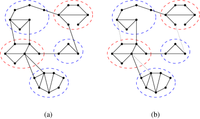
Figure 1. (a) A graph with a bipartite partition. Circles enclose vertices within the same domain.(b) The dashed edges are removed from (a) to generate a tree-partition.

We now prove that the critical points of the equipartition energy $\Lambda(\mathcal{P};\alpha)$ correspond to the eigenvectors of $H(G)$ and vice versa. The search for critical points should be carried out in the manifold $\mathcal{Q}(\mathcal{P})$. To do so we search for the critical points of $\lambda_{1}(P_{1};\alpha)$ and impose the restriction to $\mathcal{Q}(\mathcal{P})$ by introducing $(\nu-1)$ Lagrange multipliers $\{\zeta_{k}\}$. One has to search for the critical points of

(36) $$\tilde{\Lambda}(\mathcal{P};\alpha)=\lambda_{1}(P_{1};\alpha)+\sum_{k=1}^{\nu-1}\zeta_{k}\left(\lambda_{1}(P_{k};\alpha)-\lambda_{1}(P_{1};\alpha)\right),$$

The sum can be written in a more concise way as

(37) $$\tilde{\Lambda}(\mathcal{P};\alpha)=\sum_{k=1}^{\nu}c_{k}\lambda_{1}(P_{k};\alpha),$$

where the $c_{k}$ are linear in the $\zeta_{k}$. For every $e=(i,j)$ only two terms in (37) depend on the parameter $\alpha_{e}$, namely the terms corresponding to $P_{\chi(i)}$ and $P_{\chi(j)}$, where the function $\chi(\cdot)$ maps a vertex to the number of the corresponding domain. Taking the derivative with respect to $\alpha_{ij}$, we get

(38) $$\frac{\partial\tilde{\Lambda}(\mathcal{P};\alpha)}{\partial\alpha_{ij}}=c_{\chi(i)}\frac{\partial\lambda_{1}(P_{\chi(i)};\alpha)}{\partial\alpha_{ij}}+c_{\chi(j)}\frac{\partial\lambda_{1}(P_{\chi(j)};\alpha)}{\partial\alpha_{ij}}.$$

As previously, let $g(P_{k};\alpha)$ be the first eigenvector of the domain Hamiltonian $H(P_{k};\alpha)$, normalized and positive. Using first-order perturbation theory and the explicit dependence of the potential on $\alpha_{ij}$, similar to what is done in theorem 3.2 the following equations must be satisfied at the critical point for every $(i,j)\in\mathcal{E}(G)\setminus\mathcal{E(P)}$:

(39) $$c_{\chi(i)}g_{i}(P_{\chi(i)};\alpha)^{2}-c_{\chi(j)}\frac{1}{\alpha_{ij}^{2}}g_{j}(P_{\chi(j)};\alpha)^{2}=0.$$

We immediately conclude that the critical values of the Lagrange multipliers $c_{\chi}$ are non-negative. Form the function

(40) $$f=\sum_{k=1}^{\nu-1}\pm\sqrt{c_{k}}g(P_{k};\alpha),$$

where the signs are to be chosen in accordance with the bipartite structure of the partition $\mathcal{P}$. Then equation (39) can be written as

$$f_{i}^{2}-\frac{1}{\alpha_{ij}^{2}}f_{j}^{2}=0\qquad\text{or}\qquad\alpha_{ij}=\frac{f_{j}}{f_{i}},$$

which describes the values of $\alpha_{e}$ at the critical points. The function $f$ is an eigenfunction of the Hamiltonian $H(\mathcal{P},\alpha^{c})$ — in fact one belonging to the $(\nu-1)$-dimensional eigenspace of the degenerate lowest eigenvalue $\Lambda(\mathcal{P};\alpha^{c})$. It can now be shown by explicit calculation, see the discussion leading up to equation (11), that $f$ is also an eigenfunction of the original Hamiltonian $H(G)$.

Conversely, starting from an eigenfunction $f$ with the given nodal domain structure $\mathcal{P}$, we define

$$\alpha_{ij}=\frac{f_{j}}{f_{i}},\qquad c_{k}=\sum_{v\in P_{k}}f_{v}^{2},$$

and check that the condition for the critical point (39) is satisfied.

Finally, to show (35), we go back to the graph $G_{\xi}$ and start the process of successive addition of edges and use (24) at each step, since all parameters $\alpha_{e}$ are negative. Thus, the change in the position in the spectrum $\Delta n$ over $\eta$ additions equals the number of times the critical point is approached as a maximum:

$$\Delta n=\sum M(e).$$

Since at the beginning of the process we had a Courant-sharp eigenfunction with $\nu$ domains, its position in the spectrum was $\nu$. Thus the change $\Delta n$ of position is from $\nu$ to $n$, or,

(41) $$n-\nu_{n}=\mu_{n},$$

where $\mu_{n}$ is the total number of independent directions in which one approaches the critical point of the equipartition as a maximum; the Morse index (see [1, Section 4.3] for more detail).

The above construction was carried out for a particular parametrization of the manifold in the space of parameters corresponding to equipartitions. However, since $\Lambda(P;\alpha)$ is analytic in the neighborhood of the critical point, the Morse index does not depend on the choice of coordinates. ∎

5. Acknowledgements

The authors cordially thank Rami Band for many invaluable discussions and comments. The work of HR and US was supported by an EPSRC grant (EP/G02187), The Israel Science Foundation (ISF) grant (169/09) and from the Welsh Institute of Mathematical and Computational Science (WIMCS). The work of GB was suported by the National Science Foundation under Grant No. DMS-0907968. HR and GB thank the Department of Complex Systems at the Weizmann Institute for the hospitality extended during their visits.

References

- [1] R. Band, G. Berkolaiko, H. Raz, and U. Smilansky. On the connection between the number of nodal domains on quantum graphs and the stability of graph partitions. Accepted at Comm. Math. Phys., 2011.
- [2] R. Band, I. Oren, and U. Smilansky. Nodal domains on graphs - how to count them and why? In Analysis on Graphs and its Applications, Proc. Symp. Pure. Math., pages 5–28. AMS, 2008.
- [3] R. Band, T. Shapira, and U. Smilansky. Nodal domains on isospectral quantum graphs: the resolution of isospectrality? Journal of Physics A Mathematical General, 39:13999–14014, 2006.
- [4] R. Band and U. Smilansky. Resolving the isospectrality of the dihedral graphs by counting nodal domains. In Eur. Phys. J. Special Topics, volume 145, pages 171–179, 2007.
- [5] G. Berkolaiko. A lower bound for nodal count on discrete and metric graphs. Commun. Math. Phys., 278:803–819, 2007.
- [6] G. Berkolaiko, P. Kuchment, and U. Smilansky. Critical partitions and nodal deficiency of billiard eigenfunctions. preprint arXiv:1107.3489, 2011.
- [7] G. Blum, S. Gnutzmann, and U. Smilansky. Nodal domains statistics: A criterion for quantum chaos. Physical Review Letters, 88(11):114101, Mar. 2002.
- [8] E. Bogomolny, R. Dubertrand, and C. Schmit. SLE description of the nodal lines of random wave functions. J. Phys. A: Math. Theor., 40:381–395, 2007.
- [9] E. Bogomolny and C. Schmit. Percolation model for nodal domains of chaotic wave functions. Physical Review Letters, 88(11):114102, Mar. 2002.
- [10] R. Courant. Ein allgemeiner Satz zur Theorie der Eigenfunktione selbstadjungierter Differentialausdrücke. Nachr. Ges. Wiss. Göttingen Math Phys, K1, 1923.
- [11] E. B. Davies, G. M. L. Gladwell, J. Leydold, and P. F. Stadler. Discrete nodal domain theorems. Linear Algebra Appl., 336:51–60, 2001.
- [12] M. Fiedler. Eigenvectors of acyclic matrices. Czechoslovak Mathematical Journal, 25, No. 4:607–618, 1975.
- [13] S. Gnutzman, U. Smilansky, and J. Weber. Nodal counting on quantum graphs. Waves in Random Media, 14:S61–S73, 2003.
- [14] S. Gnutzmann, U. Smilansky, and N. Sondergaard. Resolving isospectral ‘drums’ by counting nodal domains. Journal of Physics A Mathematical General, 38:8921–8933, Oct. 2005.
- [15] B. Helffer, T. Hoffmann-Ostenhof, and S. Terracini. Nodal domains and spectral minimal partitions. Annales de L’Institut Henri Poincare Section Physique Theorique, 26:101–138, Jan. 2009.
- [16] R. A. Horn and C. R. Johnson. Matrix Analysis. Cambridge University Press, 1999.
- [17] D. K. J. Brüning and C. Puhle. Comment on “resolving isospectral ‘drums’ by counting nodal domains”. J. Phys. A: Math. Theor., 40:15143–15147, 2007.
- [18] P. D. Karageorge and U. Smilansky. Counting nodal domains on surfaces of revolution. J. Phys. A: Math. Theor., 41:205102, 2008.
- [19] D. Klawonn. Inverse nodal problems. J. Phys. A: Math. Theor., 42:175209, Aug. 2009.
- [20] I. Oren. Nodal domain counts and the chromatic number of graphs. J. Phys. A: Math. Theor., 40:9825–9832, 2007.
- [21] A. Pleijel. Remarks on Courant’s nodal line theorem. Communications on Pure and Applied Mathematics, 9(3):543–550, 1956.
- [22] I. Polterovich. Pleijel’s nodal domain theorem for free membranes. Proc. Amer. Math. Soc., 137(3):1021–1024, 2009.