Gaussian semiparametric estimates on the unit sphere

Abstract

We study the weak convergence (in the high-frequency limit) of the parameter estimators of power spectrum coefficients associated with Gaussian, spherical and isotropic random fields. In particular, we introduce a Whittle-type approximate maximum likelihood estimator and we investigate its asympotic weak consistency and Gaussianity, in both parametric and semiparametric cases.

, and

1 Introduction

The purpose of this paper is to investigate the asymptotic behavior of a Whittle-like approximate maximum likelihood procedure for the estimation of the spectral parameters (e.g., the spectral index) of isotropic Gaussian random fields defined on the unit sphere $\mathbb{S}^{2}$. In our approach, we consider the expansion of the field into spherical harmonics, that is, we implement a form of Fourier analysis on the sphere, and we implement approximate maximum likelihood estimates under both parametric and semiparametric assumptions on the behavior of the angular power spectrum. We stress that the asymptotic framework we are considering here is rather different from usual – in particular, we assume we are observing a single realization of an isotropic field, the asymptotics being with respect to higher and higher resolution data becoming available (i.e., higher and higher frequency components being observed). In some sense, then the issues we are considering are related to the growing area of fixed-domain asymptotics (see, e.g., [1, 25]). From the point of view of the proofs, on the other hand, our arguments are in some cases reminiscent of those entertained, for instance, by [37], where semiparametric estimates of the long memory parameter for covariance stationary processes are analyzed; see also [14] for related results in the setting of anisotropic random fields.

In our assumptions, we do not impose a priori a parametric model on the dependence structure of the random field we are analyzing; we rather impose various forms of regularly varying conditions, which only constrain the high-frequency behaviour of the angular power spectrum. We are able to show consistency under the least restrictive assumptions; a central limit theorem holds under more restrictive conditions, while asymptotic Gaussianity can be established under general conditions for a slightly-modified (narrow-band) procedure, entailing a loss of a logarithmic factor in the rate of convergence. Our analysis is strongly motivated by applications, especially in a Cosmological framework (see, e.g., [9, 8]); in this area, huge datasets on isotropic, spherical random fields (usually assumed to be Gaussian) are currently being collected and made publicly available by celebrated satellite missions such as WMAP or Planck (see, e.g., http://map.gsfc.nasa.gov/); parameter estimation of the spectral index and other spectral parameters has been considered by many authors (see, e.g., [15] for a review), but no rigorous asymptotic result has so far been produced, to the best of our knowledge. We thus hope that the consistency and asymptotic Gaussianity properties we provide for our Whittle-like procedure may provide a contribution toward further developments. We refer also to [3, 4, 12, 13, 35, 34, 27] for further theoretical and applied results on angular power spectrum estimation, in a purely nonparametric setting, and to [18, 20, 19, 17, 11, 16, 23, 21, 28] for further results on statistical inference for spherical random fields. Fixed-domain asymptotics for the tail behaviour of the spectral density on Euclidean spaces has been recently considered also by [14, 2] and [41]; the issue is of great interest, for instance, in connection with kriging techniques for geophysical data analysis, see [39] for a textbook reference.

The plan of the paper is as follows: in Section 2, we will recall briefly some well-known background material on harmonic analysis for spherical isotropic random fields; in Section 3 we introduce Whittle-like maximum pseudo-likelihood estimators for angular power spectrum coefficients based on spherical harmonics; Section 4 is devoted to the asymptotic results, while in Section 5 we investigate narrow-band estimates. The presence of observational noise is considered in Section 6, while Section 7 provides some numerical evidence to validate the findings of the paper. Directions for future research are discussed in Section 8, while some auxiliary technical results are collected in the Appendix.

2 Spherical random fields and angular power spectrum

In this section, we will present some well-known background results concerning harmonic analysis on the sphere. We shall focus on zero-mean, isotropic Gaussian random fields $T\mathchoice{\nobreak\,\colon}{\nobreak\,\colon}{\nobreak\,\colon\;}{\nobreak\,\colon\;}\mathbb{S}^{2}\times\Omega\rightarrow\mathbb{R}$. It is well known that such fields can be given a spectral representation such that

$$T(x) = \sum_{l\geq 0}\sum_{m=-l}^{l}a_{lm}Y_{lm}(x)=\sum_{l\geq 0}T_{l}(x),$$ (1)

$$a_{lm} = \int_{\mathbb{S}^{2}}T(x)\overline{Y}_{lm}(x)\,\mathrm{d}x,$$ (2)

where the set of homogenous polynomials $\{Y_{lm}\mathchoice{\nobreak\,\colon}{\nobreak\,\colon}{\nobreak\,\colon\;}{\nobreak\,\colon\;}l\geq 0,m=-l,\ldots,l\}$ represents an orthonormal basis for the space $L^{2}(\mathbb{S}^{2},\mathrm{d}x)$, the class of functions defined on the unitary sphere which are square-integrable with respect to the measure $\mathrm{d}x$ (see, e.g., [38, 16, 28], for more details, and [24, 26] for extensions). Note that this equality holds in both $L^{2}(\mathbb{S}^{2}\times\Omega,\mathrm{d}x\otimes\mathbb{P})$ and $L^{2}(\mathbb{P})$ senses for every fixed $x\in\mathbb{S}^{2}$. We recall also that a field $T(\cdot)$ is isotropic if and only if for every $g\in SO(3)$ (the special group of rotations in $\mathbb{R}^{3}$) and $x\in\mathbb{S}^{2}$ (the unit sphere), we have

$$T(x)\stackrel{{\scriptstyle d}}{{=}}T(gx),$$

where the equality holds in the sense of processes.

An explicit form for spherical harmonics is given in spherical coordinates $\vartheta\in[0,\uppi]$, $\varphi\in[0,2\uppi)$ by:

$$Y_{lm}(\vartheta,\varphi) = \sqrt{\frac{2l+1}{4\uppi}\frac{(l-m)!}{(l+m)!}}P_{lm}(\cos\vartheta)\mathrm{e}^{\mathrm{i}m\varphi}\qquad\mbox{for }m\geq 0,$$

$$Y_{lm}(\vartheta,\varphi) = (-1)^{m}\overline{Y}_{l,-m}(\vartheta,\varphi)\qquad\mbox{for }m<0,$$

$P_{lm}(\cos\vartheta)$ denoting the associated Legendre function; for $m=0$, we have $P_{l0}(\cos\vartheta)=P_{l}(\cos\vartheta)$, the standard set of Legendre polynomials (see again [38, 28]). The following orthonormality property holds:

$$\int_{\mathbb{S}^{2}}Y_{lm}(x)\overline{Y}_{l^{\prime}m^{\prime}}(x)\,\mathrm{d}x=\delta_{l}^{l^{\prime}}\delta_{m}^{m^{\prime}}.$$

For an isotropic Gaussian field, the spherical harmonics coefficients $a_{lm}$ are Gaussian complex random variables such that

$$\mathbb{E}(a_{lm})=0,\qquad\mathbb{E}(a_{l_{1}m_{2}}\overline{a}_{l_{2}m_{2}})=\delta_{l_{2}}^{l_{1}}\delta_{m_{2}}^{m_{1}}C_{l},$$

where of course the angular power spectrum $C_{l}$ fully characterizes the dependence structure under Gaussianity; here, $\delta_{a}^{b}$ is the Kronecker delta, taking value one for $a=b$, zero otherwise. Further characterizations of the spherical harmonics coefficients are provided, for instance, by [5, 28]; here we simply recall that

$$\frac{a_{l0}^{2}}{C_{l}}\sim\chi_{1}^{2}\qquad\mbox{for }m=0,\qquad\frac{2|a_{lm}|^{2}}{C_{l}}\sim\chi_{2}^{2}\qquad\mbox{for }m=\pm 1,\pm 2,\ldots,\pm l,$$

where all these random variables are independent. Given a realization of the random field, an estimator of the angular power spectrum can be defined as:

$$\widehat{C}_{l}=\frac{1}{2l+1}\sum_{m=-l}^{l}|a_{lm}|^{2},$$ (3)

the so-called empirical angular power spectrum. It is immediately seen that

$$\mathbb{E}\widehat{C}_{l}=\frac{1}{2l+1}\sum_{m=-l}^{l}C_{l}=C_{l},\qquad\operatorname{Var}\biggl{(}\frac{\widehat{C}_{l}}{C_{l}}\biggr{)}=\frac{2}{2l+1}\rightarrow 0\qquad\mbox{for }l\rightarrow+\infty.$$

We shall now focus on some semiparametric models on the angular power spectrum; here, by semiparametric we mean that we shall assume a parametric form on the asymptotic behavior of $C_{l}$, but we shall refrain from a full characterization over all multipoles $l$. More precisely, we formulate the following:

Condition 1.

The random field $T(x)$ is Gaussian and isotropic with angular power spectrum such that:

$$C_{l}=G(l)l^{-\alpha_{0}}>0,$$ (4)

where $\alpha_{0}>2$ and for all $l=1,2,\ldots$

$$0<c_{1}\leq G(l)\leq c_{2}<+\infty.$$

Condition 1 seems very mild, as it is basically requiring only some form of regular variation on the tail behavior of the angular power spectrum $C_{l}$. For instance, in the CMB framework the so-called Sachs–Wolfe power spectrum (i.e., the leading model for fluctuations of the primordial gravitational potential) takes the form (4), the spectral index $\alpha_{0}$ capturing the scale invariance properties of the field itself ($\alpha_{0}$ is expected to be close to 2 from theoretical considerations, a prediction so far in good agreement with observations, see, e.g., [9] and [22]). For our asymptotic results below, we shall need to strengthen it somewhat; as we shall see, Condition 2 will turn out to be sufficient to establish a rate of convergence for our estimator, under Condition 3 we will be able to provide a Law of Large Numbers, while under Condition 4 our estimates will be shown to be asymptotically Gaussian and centered, thus making statistical inference feasible. On the other hand, in Section 5 we shall be able to provide narrow-band estimates with asymptotically centred limiting Gaussian law under Condition 2, to the price of a logarithmic term in the rate of convergence. Of course, the conditions below are nested, that is, Condition 4 implies Condition 3, which trivially implies Condition 2.

Condition 2.

Condition 1 holds and moreover, $G(l)$ satisfies the smoothness condition

$$G(l)=G_{0}\biggl{\{}1+\mathrm{O}\biggl{(}\frac{1}{l}\biggr{)}\biggr{\}}.$$

Condition 3.

Condition 2 holds and moreover, $G(l)$ satisfies

$$G(l)=G_{0}\biggl{\{}1+\frac{\kappa}{l}+\mathrm{o}\biggl{(}\frac{1}{l}\biggr{)}\biggr{\}}.$$

Condition 4.

Condition 3 holds with $\kappa=0$, that is, $G(l)$ satisfies the smoothness condition

$$G(l)=G_{0}\biggl{\{}1+\mathrm{o}\biggl{(}\frac{1}{l}\biggr{)}\biggr{\}}.$$

A straightforward example that satisfies the previous assumptions is provided by the rational function

$$G(l)=\frac{\Pi_{1}(l)}{\Pi_{2}(l)}=\frac{p_{k}l^{k}+\cdots+p_{1}l+p_{0}}{q_{k}l^{k}+\cdots+q_{1}l+pq},$$ (5)

where $\Pi_{1}(l)$ and $\Pi_{2}(l)$ are positive valued polynomials of order $k\in\mathbb{N}$, such that:

$$0<c_{1}\leq\frac{\Pi_{1}(l)}{\Pi_{2}(l)}\leq c_{2}<+\infty.$$

Clearly (5) satisfies Condition 3 (and hence Condition 2) for

$$G_{0}=\frac{p_{k}}{q_{k}}\quad\mbox{and}\quad\kappa=\frac{p_{k-1}}{p_{k}}-\frac{q_{k-1}}{q_{k}};$$

Condition 4 is satisfied when $p_{k-1}=q_{k-1}=0$, or, more generally, for $\frac{p_{k-1}}{p_{k}}=\frac{q_{k-1}}{q_{k}}$.

3 A Whittle-like approximation to the likelihood function

Our aim in this section is to discuss heuristically a Whittle-like approximation for the log-likelihood of isotropic spherical Gaussian fields, and to derive the corresponding estimator. Assume that the triangular array $\{a_{lm}\}$, $m=-l,\ldots,l$, $l=1,2,\ldots,L$, is evaluated from the observed field $\{T(x)\}$, by means of (2). Our motivating rationale is the idea that a set of harmonic components up to multipole $L$ can be reconstructed without observational noise or numerical error, whereas the following are simply discarded; this is clearly a simplified picture, but we believe it provides an accurate approximation to many current experimental set-ups. Of course, $L$ grows larger when more sophisticated experiments are run ($L$ can be considered in the order of $500/600$ for data collected from WMAP and $1500/2000$ for those from Planck). It is readily seen from (3) that

$$\widehat{C}_{l}=\frac{1}{2l+1}\Biggl{\{}a_{l0}^{2}+2\sum_{m=1}^{l}\bigl{[}\Re\{a_{lm}\}\bigr{]}^{2}+2\sum_{m=1}^{l}\bigl{[}\Im\{a_{lm}\}\bigr{]}^{2}\Biggr{\}},$$

where the variables $\{a_{l0},\sqrt{2}\Re\{a_{l1}\},\sqrt{2}\Im\{a_{l1}\},\ldots,\sqrt{2}\Re\{a_{ll}\},\sqrt{2}\Im\{a_{ll}\}\}$ are i.i.d. Gaussian variables with law $\mathcal{N}(0,C_{l})$, see [5]. The likelihood function can then be written down as

$$-2\log\mathcal{L}_{l}\bigl{(}\theta;\{a_{lm}\}_{m=-l}^{l}\bigr{)}=\mathrm{const}+(2l+1)\frac{\widehat{C}_{l}}{C_{l}(\theta)}-(2l+1)\log\frac{\widehat{C}_{l}}{C_{l}(\theta)}.$$

Clearly this landscape is overly simplified, for instance, due to numerical errors and aliasing effects the expected value $\mathbb{E}|a_{lm}|^{2}$ may not be exactly equal to the population model $C_{l}(\theta)$; however in Conditions 1 and following we are allowing the two to differ to various degrees, and we expect this to cover to some of effect these experimental features that we are neglecting. Also, rather than a sharp cutoff at $L$, a smooth transition toward noisier frequencies would represent more efficiently actual experimental circumstances; we shall address this issue later on in this paper. Finally, it may be unreasonable to assume that the spherical surface is fully observed; for most experimental set-ups, either in Cosmology or in Geophysics, only subsets are actually sampled. This problem can be addressed by focussing on wavelet transforms rather than standard Fourier analysis; we shall consider this extension in a different work.

An alternative heuristics for our framework can be introduced considering that for $l=1,2,\ldots,L$, the following Fourier components can be observed on a discrete grid of points $\{x_{1},\ldots,x_{K}\}$

$$\accentset{\longrightarrow}{T}_{l}=\bigl{\{}T_{l}(x_{1}),\ldots,T_{l}(x_{k}),\ldots,T_{l}(x_{K})\bigr{\}}.$$

To simplify our discussion, we shall also pretend that $\mathcal{X}_{k}:=\{x_{1},\ldots,x_{K}\}$ form a set of approximate cubature points with constant cubature weights $\lambda_{k}=4\uppi/K$ (see, e.g., [30, 31]), so that we have

$$\sum_{k}\frac{4\uppi}{K}Y_{lm_{1}}(x_{k})\overline{Y}_{lm_{2}}(x_{k})\simeq\delta_{m_{1}}^{m_{2}}\qquad\mbox{for }l=1,2,\ldots,L.$$

As discussed also by [4], the number of cubature points must grow at least as quickly as the square of the highest multipole considered, that is, $L^{2}=\mathrm{O}(\operatorname{card}(\mathcal{X}_{k}))$. For instance, for a satellite experiment such as Planck the pixelization has cardinality of order $5\times 10^{6}$, and the highest multipole that can be analyzed correspond broadly to the order $l=2\times 10^{3}$. As before, this landscape is overly simplified; for instance, cubature weights on the sphere are known not to be constant, but their variation is usually considered numerically negligible.

The frequency components $T_{l}$ are well known to be independent and we can hence write down the likelihood function as

$$\mathcal{L}(\theta;T):=\prod_{l=1}^{L}\mathcal{L}_{l}(\theta;\accentset{\longrightarrow}{T}_{l}),$$

where

$$\mathcal{L}_{l}(\theta;\accentset{\longrightarrow}{T}_{l}) = (2\uppi)^{-(2l+1)/2}\Omega_{l}^{-1/2}\exp\biggl{\{}-\frac{1}{2}\accentset{\longrightarrow}{T}_{l}^{\prime}\Omega_{l}^{-1}\accentset{\longrightarrow}{T}_{l}\biggr{\}},$$

$$\{\Omega_{l}\}_{jk} = \biggl{\{}\Omega_{l}(x_{j},x_{k})=\frac{2l+1}{4\uppi}C_{l}P_{l}\bigl{(}\langle x_{j},x_{k}\rangle\bigr{)}\biggr{\}}.$$

The matrix $\Omega_{l}$ can be (approximately) decomposed as follows:

$$\Omega_{l} \simeq \sqrt{\frac{4\uppi}{K}}\left[\matrix{Y_{l,-l}(x_{1})&Y_{l,-l+1}(x_{1})&\cdots&Y_{l,l}(x_{1})\cr Y_{l,-l}(x_{2})&\cdots&\cdots&Y_{l,l}(x_{2})\cr\vdots&\vdots&\vdots&\vdots\cr Y_{l,-l}(x_{K})&Y_{l,-l+1}(x_{K})&\cdots&Y_{l,l}(x_{K})}\right]$$

$${}\times\frac{K}{4\uppi}C_{l}I_{2l+1}\times\sqrt{\frac{4\uppi}{K}}\left[\matrix{\overline{Y}_{l,-l}(x_{1})&\overline{Y}_{l,-l}(x_{2})&\cdots&\overline{Y}_{l,-l}(x_{K})\cr\overline{Y}_{l,-l+1}(x_{1})&\cdots&\cdots&\overline{Y}_{l,-l+1}(x_{K})\cr\vdots&\vdots&\vdots&\vdots\cr\overline{Y}_{l,l}(x_{1})&\overline{Y}_{l,l}(x_{2})&\cdots&\overline{Y}_{l,l}(x_{K})}\right]$$

$$= \!\!:\mathcal{Y}_{l}\times C_{l}(\theta)I_{2l+1}\times\mathcal{Y}_{l}^{\ast}.$$

In fact

$$\mathcal{Y}_{l}^{\ast}\mathcal{Y}_{l}\simeq I_{2l+1}\quad\mbox{and}\quad\det\{\Omega_{l}\}\simeq C_{l}^{2l+1}(\theta).$$

Hence,

$$-2\log\mathcal{L}_{l}(\theta;\accentset{\longrightarrow}{T}_{l})\simeq K+(2l+1)\log C_{l}(\theta)+\bigl{\{}\accentset{\longrightarrow}{T}_{l}^{\prime}\mathcal{Y}_{l}\times C_{l}^{-1}(\theta)I_{2l+1}\times\mathcal{Y}_{l}^{\ast}\accentset{\longrightarrow}{T}_{l}\bigr{\}}.$$

Now

$$\mathcal{Y}_{l}^{\ast}\accentset{\longrightarrow}{T}_{l} = \sqrt{\frac{4\uppi}{K}}\left[\matrix{\overline{Y}_{l,-l}(x_{1})&\overline{Y}_{l,-l}(x_{2})&\cdots&\overline{Y}_{l,-l}(x_{K})\cr\overline{Y}_{l,-l+1}(x_{1})&\cdots&\cdots&\overline{Y}_{l,-l+1}(x_{K})\cr\vdots&\vdots&\vdots&\vdots\cr\overline{Y}_{l,l}(x_{1})&\overline{Y}_{l,l}(x_{2})&\cdots&\overline{Y}_{l,l}(x_{K})}\right]$$

$${}\times\left[\matrix{\sum_{m}a_{lm}Y_{lm}(x_{1})\cr\sum_{m}a_{lm}Y_{lm}(x_{2})\cr\vdots\cr\sum_{m}a_{lm}Y_{lm}(x_{K})}\right]$$

$$= \sqrt{\frac{4\uppi}{K}}\left[\matrix{\sum_{m_{1}}a_{lm_{1}}\sum_{k}Y_{lm_{1}}(x_{k})\overline{Y}_{l,-l}(x_{k})\cr\sum_{m_{1}}a_{lm_{1}}\sum_{k}Y_{lm_{1}}(x_{k})\overline{Y}_{l,-l+1}(x_{k})\cr\vdots\cr\sum_{m_{1}}a_{lm_{1}}\sum_{k}Y_{lm_{1}}(x_{k})\overline{Y}_{l,l}(x_{k})}\right]$$

$$\simeq \sqrt{\frac{K}{4\uppi}}\left[\matrix{a_{l,-l}\cr a_{l,-l+1}\cr\vdots\cr a_{l,l}}\right],$$

whence

$$\biggl{\{}\accentset{\longrightarrow}{T}_{l}^{\prime}\mathcal{Y}_{l}\times\frac{4\uppi}{K}\frac{1}{C_{l}(\theta)}I_{2l+1}\times\mathcal{Y}_{l}^{\ast}\accentset{\longrightarrow}{T}_{l}\biggr{\}}\simeq\sum_{m}\frac{|a_{lm}|^{2}}{C_{l}(\theta)}=(2l+1)\frac{\widehat{C}_{l}}{C_{l}(\theta)}.$$

As before, we can then conclude heuristically that

$$-2\log\mathcal{L}_{l}(\theta;\accentset{\longrightarrow}{T}_{l})\simeq\mathrm{const}+(2l+1)\frac{\widehat{C}_{l}}{C_{l}(\theta)}-(2l+1)\log\frac{\widehat{C}_{l}}{C_{l}(\theta)}.$$ (6)

Again we stress that for a general spherical random field with an infinite-terms expansion such as (1) the relationship (6) cannot hold exactly; indeed, precise cubature formulae can be established only for finite order spherical harmonics. In general, this may introduce some numerical error: as mentioned before, however, we pretend in this paper that such correction factors are covered by Conditions 1–4. In other words, we envisage a situation where data analysis is carried over on multipoles $l$ where numerical errors are of smaller order and the approximation (4) holds for the expected variance of the sample coefficients $\{a_{lm}\}$.

4 Asymptotic results: Consistency and asymptotic Gaussianity

As motivated in the Introduction, in this paper we shall not assume we have actually available a fully parametric model for the angular power spectrum. Instead, the idea will be to use an approximate maximum likelihood estimator, which shall exploit the asymptotic approximation provided by Condition 1, that is, $C_{l}\simeq Gl^{-\alpha}$. In view of the discussion in the previous section, the following Definition seems rather natural:

Definition 1.

The Spherical Whittle estimator for the parameters $(\alpha_{0},G_{0})$ is provided by

$$(\widehat{\alpha}_{L},\widehat{G}_{L}):=\arg\min_{\alpha\in A,G\in(0,\infty)}\sum_{l=1}^{L}\biggl{\{}(2l+1)\frac{\widehat{C}_{l}}{Gl^{-\alpha}}-(2l+1)\log\frac{\widehat{C}_{l}}{Gl^{-\alpha}}\biggr{\}}.$$

Remark 1.

For general parametric models $C_{l}=C_{l}(\vartheta)$, the Spherical Whittle estimator for a parameter $\vartheta\in\Theta\subset\mathbb{R}^{p}$ can be obviously defined as

$$\widehat{\vartheta}_{L}:=\arg\min_{\vartheta\in\Theta}\sum_{l=1}^{L}\biggl{\{}(2l+1)\frac{\widehat{C}_{l}}{C_{l}(\vartheta)}-(2l+1)\log\frac{\widehat{C}_{l}}{C_{l}(\vartheta)}\biggr{\}}.$$

Remark 2.

To ensure that the estimator exists, as usual we shall assume throughout this paper that the parameter space for $\alpha$ is a compact subset of $\mathbb{R}$; more precisely we take $\alpha\in A=[a_{1},a_{2}]$, $2<a_{1}<a_{2}<\infty$, and $G\in(0,\infty)$. This is little more than a formal requirement that is standard in the literature on (pseudo-)maximum likelihood estimation. It should be noted that Spherical Whittle estimates are computationally extremely convenient, while their counterpart in the real domain is for all practical purposes unfeasible, given the dimension of current datasets.

Remark 3.

Under Condition 4, it is readily seen that $(2l+1)\widehat{C}_{l}/Gl^{-\alpha_{0}}$ is asymptotically distributed as a Gamma random variables of parameters $\{2l+1,1\}$, and the Spherical Whittle estimator is asymptotically equivalent to exact maximum likelihood.

We can rewrite in a more transparent form the previous estimator following an argument analogous to [37], that is, “concentrating out” the parameter $G$. Indeed, the previous minimization problem is equivalent to let us consider

$$(\widehat{\alpha}_{L},\widehat{G}_{L}) := \arg\min_{\alpha,G}\mathcal{R}_{L}(G,\alpha),$$

$$\mathcal{R}_{L}(G,\alpha) := \sum_{l=1}^{L}(2l+1)\frac{\widehat{C}_{l}}{Gl^{-\alpha}}+\sum_{l=1}^{L}(2l+1)\log G$$

$${}+\sum_{l=1}^{L}(2l+1)\log l^{-\alpha}.$$

Simple computations show that the minimization problem can be equivalently reformulated as

$$\widehat{\alpha}_{L} = \arg\min_{\alpha}R_{L}(\alpha),$$

$$R_{L}(\alpha) = \Biggl{(}\log\widehat{G}(\alpha)-\frac{\alpha}{\sum_{l=1}^{L}(2l+1)}\sum_{l=1}^{L}(2l+1)\log l\Biggr{)}.$$

The proof of the following result is quite standard and goes largely along the lines of an analogous results provided in [37]. As most of the ones to follow, is delayed to the Appendix.

Theorem 1

Under Condition 1, as $L\rightarrow\infty$ we have

$$\widehat{\alpha}_{L}\rightarrow_{p}\alpha_{0};$$

moreover, under Condition 2,

$$\widehat{G}_{L}\rightarrow_{p}G_{0}.$$

Next step is the investigation of the asymptotic distribution. To this aim, we shall exploit some classical argument on asymptotic Gaussianity for extremum estimates, as recalled, for instance, by [32], Theorem 3.1.

Theorem 2

Let $\widehat{\alpha}_{L}=\arg\min_{\alpha\in A}R_{L}(\alpha)$ defined as in (4).

(

• a)]

• Under Condition 2 we have that

  $$\bigl{\{}\mathbb{E}(\widehat{\alpha}_{L}-\alpha_{0})^{2}\bigr{\}}^{1/2}=\mathrm{O}\biggl{(}\frac{\log L}{L}\biggr{)}\qquad\mbox{whence }(\widehat{\alpha}_{L}-\alpha_{0})=\mathrm{O}_{p}\biggl{(}\frac{\log L}{L}\biggr{)}\qquad\mbox{as }L\rightarrow\infty.$$ (8)

• Under Condition 3 we have that

  $$\frac{L}{4\log L}(\widehat{\alpha}_{L}-\alpha_{0})\longrightarrow_{p}-\kappa.$$ (9)

• Under Condition 4 we have that

  $$\frac{\sqrt{2}L}{4}(\widehat{\alpha}_{L}-\alpha_{0})\stackrel{{\scriptstyle d}}{{\longrightarrow}}\mathcal{N}(0,1).$$ (10)

Proof.

We note first that under Condition 4, (10) is an immediate consequence of (9); on the other hand, the proof of (8) follows on exactly the same lines as (9), the only difference here being that the asymptotic bias term cannot be given an analytic expression but only bounded. It is then sufficient to establish (9), as we shall do below.

Following the notation introduced above, for each $L$ there exists $\overline{\alpha}_{L}\in(\alpha_{0}-\widehat{\alpha},\alpha_{0}+\widehat{\alpha})$ such that, with probability one:

$$(\widehat{\alpha}_{L}-\alpha_{0})=-\frac{S_{L}(\alpha_{0})}{Q_{L}(\overline{\alpha}_{L})},$$

where $S_{L}(\alpha)$ is the score function corresponding to $R_{L}(\alpha)$, given by:

$$S_{L}(\alpha)=\frac{\mathrm{d}}{\mathrm{d}\alpha}R(\alpha)=\frac{\widehat{G}_{1}(\alpha)}{\widehat{G}(\alpha)}-\frac{1}{\sum_{l=1}^{L}(2l+1)}\sum_{l=1}^{L}(2l+1)\log l$$

and

$$Q_{L}(\alpha) = \frac{\mathrm{d}}{\mathrm{d}\alpha}S_{L}(\alpha)=\frac{\mathrm{d}^{2}}{\mathrm{d}\alpha^{2}}R(\alpha)=\frac{\widehat{G}_{2}(\alpha)\widehat{G}(\alpha)-\widehat{G}_{1}^{2}(\alpha)}{\widehat{G}{}^{2}(\alpha)}$$

$$= \Biggl{(}\sum_{l=1}^{L}(2l+1)\bigl{(}\log^{2}l\bigr{)}\frac{\widehat{C}_{l}}{l^{-\alpha}}\Biggl{\{}\sum_{l=1}^{L}(2l+1)\frac{\widehat{C}_{l}}{l^{-\alpha}}\Biggr{\}}-\Biggl{\{}\sum_{l=1}^{L}(2l+1)(\log l)\frac{\widehat{C}_{l}}{l^{-\alpha}}\Biggr{\}}^{2}\Biggr{)}$$

$${}\Big{/}\Biggl{\{}\sum_{l=1}^{L}(2l+1)\frac{\widehat{C}_{l}}{l^{-\alpha}}\Biggr{\}}^{2},$$

where $\widehat{G}(\alpha)$, $\widehat{G}_{1}(\alpha)$, $\widehat{G}_{2}(\alpha)$ are, respectively, the estimate of $G$ and its first and second derivatives, as in Lemma 5. By direct substitution, we have immediately:

$$S_{L}(\alpha)=\frac{1}{\sum_{l=1}^{L}(2l+1)}\sum_{l=1}^{L}(2l+1)\log l\biggl{\{}\frac{\widehat{C}_{l}}{\widehat{G}(\alpha)l^{-\alpha}}-1\biggr{\}}.\vspace*{-1pt}$$

Now,

$$S_{L}(\alpha_{0}) = \frac{G_{0}}{\widehat{G}(\alpha_{0})}\frac{1}{\sum_{l=1}^{L}(2l+1)}\sum_{l=1}^{L}(2l+1)\log l\biggl{\{}\frac{\widehat{C}_{l}}{G_{0}l^{-\alpha_{0}}}-\frac{\widehat{G}(\alpha_{0})}{G_{0}}\biggr{\}}$$

$$= \frac{G_{0}}{\widehat{G}(\alpha_{0})}\overline{S}_{L}(\alpha_{0}),\vspace*{-1pt}$$

where

$$\overline{S}_{L}(\alpha_{0})=\frac{1}{\sum_{l=1}^{L}(2l+1)}\sum_{l=1}^{L}(2l+1)\log l\biggl{\{}\frac{\widehat{C}_{l}}{G_{0}l^{-\alpha_{0}}}-1\biggr{\}}$$

and

$$\frac{G_{0}}{\widehat{G}(\alpha_{0})}=1+\mathrm{o}_{p}(1)\qquad\mbox{as }L\rightarrow\infty$$

in view of Lemma 5. Also

$$\mathbb{E}\overline{S}_{L}(\alpha_{0}) = \frac{1}{\sum_{l=1}^{L}(2l+1)}\sum_{l=1}^{L}(2l+1)\log l\biggl{\{}\frac{C_{l}}{G_{0}l^{-\alpha_{0}}}-1\biggr{\}}$$

$$= \frac{\kappa}{\sum_{l=1}^{L}(2l+1)}\sum_{l=1}^{L}(2l+1)\frac{\log l}{l}+\mathrm{o}\biggl{(}\frac{\log L}{L}\biggr{)}=\mathrm{O}\biggl{(}\frac{\log L}{L}\biggr{)}\rightarrow 0$$

and

$$\lim_{L\rightarrow\infty}2L^{2}\operatorname{Var}\bigl{\{}\overline{S}_{L}(\alpha_{0})\bigr{\}}=1.$$ (11)

In fact, we have:

$$\operatorname{Var}\bigl{\{}\overline{S}_{L}(\alpha_{0})\bigr{\}}=V_{1}+V_{2}+V_{3},$$

where

$$V_{1} = \biggl{\{}\frac{1}{\sum_{l=1}^{L}(2l+1)}\biggr{\}}^{2}\sum_{l=1}^{L}(2l+1)^{2}(\log l)^{2}\operatorname{Var}\biggl{\{}\frac{\widehat{C}_{l}}{G_{0}l^{-\alpha_{0}}}\biggr{\}}$$

$$= \biggl{(}\frac{1}{\sum_{l=1}^{L}(2l+1)}\biggr{)}^{2}2\sum_{l=1}^{L}(2l+1)(\log l)^{2};$$

$$V_{2} = \biggl{\{}\frac{1}{\sum_{l=1}^{L}(2l+1)}\biggr{\}}^{2}\Biggl{(}\sum_{l=1}^{L}(2l+1)\log l\Biggr{)}^{2}\operatorname{Var}\biggl{(}\frac{\widehat{G}(\alpha_{0})}{G_{0}}\biggr{)};$$

$$V_{3} = \frac{-2}{\sum_{l}(2l+1)}\sum_{l=1}^{L}(2l+1)\log l\operatorname{Cov}\biggl{(}\frac{\widehat{C}_{l}}{C_{l}},\frac{\widehat{G}(\alpha_{0})}{G_{0}}\biggr{)}\cdot\frac{-2}{\sum_{l}(2l+1)}\sum_{l=1}^{L}(2l+1)\log l.$$

Now because

$$\operatorname{Var}\biggl{(}\frac{\widehat{G}(\alpha_{0})}{G_{0}}\biggr{)} = \biggl{\{}\frac{1}{\sum_{l=1}^{L}(2l+1)}\biggr{\}}^{2}\sum_{l=1}^{L}(2l+1)^{2}\operatorname{Var}\biggl{\{}\frac{\widehat{C}_{l}}{G_{0}l^{-\alpha_{0}}}\biggr{\}}$$

$$= \frac{2}{\sum_{l=1}^{L}(2l+1)};$$

$$\operatorname{Cov}\biggl{(}\frac{\widehat{C}_{l}}{C_{l}},\frac{\widehat{G}(\alpha_{0})}{G_{0}}\biggr{)} = \frac{1}{\sum_{l^{\prime}=1}^{L}(2l^{\prime}+1)}\sum_{l^{\prime}=1}^{L}\bigl{(}2l^{\prime}+1\bigr{)}\operatorname{Cov}\biggl{(}\frac{\widehat{C}_{l}}{C_{l}},\frac{\widehat{C}_{l^{\prime}}}{C_{l^{\prime}}}\biggr{)}$$

$$= \frac{2}{\sum_{l^{\prime}=1}^{L}(2l+1)};$$

we have

$$\operatorname{Var}\bigl{\{}\overline{S}_{L}(\alpha_{0})\bigr{\}} = \frac{2}{(\sum_{l=1}^{L}(2l+1))^{3}}\Biggl{(}\sum_{l=1}^{L}(2l+1)\sum_{l=1}^{L}(2l+1)(\log l)^{2}-\Biggl{(}\sum_{l=1}^{L}(2l+1)\log l\Biggr{)}^{2}\Biggr{)}$$

$$= \frac{2}{L^{6}}\frac{L^{4}}{4}=\frac{1}{2L^{2}}$$

by using (22) and (21) with $s=0$ to obtain (11). In order to establish the central limit theorem, it is sufficient to perform a careful analysis of fourth-order cumulants (note our statistics belong to the second-order Wiener chaos with respect to a Gaussian white noise random measure). Write:

$$LS_{L}(\alpha_{0})=\frac{1}{L+\mathrm{O}_{L}(1)}\sum_{l}(A_{l}+B_{l}),$$

where

$$A_{l} = (2l+1)\log l\biggl{\{}\frac{\widehat{C}_{l}}{C_{l}}-1\biggr{\}},$$ (14)

$$B_{l} = (2l+1)\log l\biggl{\{}\frac{\widehat{G}_{L}(\alpha_{0})}{G_{0}}-1\biggr{\}}.$$ (15)

In the Appendix, we show that

$$\frac{1}{L^{4}}\operatorname{cum}\biggl{\{}\sum_{l_{1}}(A_{l_{1}}+B_{l_{1}}),\sum_{l_{2}}(A_{l_{2}}+B_{l_{2}}),\sum_{l_{3}}(A_{l_{3}}+B_{l_{3}}),\sum_{l_{4}}(A_{l_{4}}+B_{l_{4}})\biggr{\}}=\mathrm{O}_{L}\biggl{(}\frac{\log^{4}L}{L^{2}}\biggr{)},$$

whence the central limit theorem follows easily from results in [33]. Indeed, using recent results from the latter authors a stronger result follows, that is,

$$d_{\mathrm{TV}}\Biggl{(}\sum_{l=1}^{L}X_{l;L},Z\Biggr{)}=\mathrm{O}\biggl{(}\frac{1}{L}\biggr{)},\qquad Z\stackrel{{\scriptstyle d}}{{=}}\mathcal{N}(0,1),$$

where $d_{\mathrm{TV}}(W,V)$ denotes the total variation distance between the random variables $W,V$, that is,

$$d_{\mathrm{TV}}(W,V)=\sup_{x}\bigl{|}\Pr\{W\in B\}-\Pr\{V\in B\}\bigr{|}\qquad\mbox{any Borel set }B.$$

Also

$$\frac{L}{\log L}\mathbb{E}\overline{S}_{L}(\alpha_{0})=\kappa\frac{L}{\sum_{l=1}^{L}(2l+1)}\sum_{l=1}^{L}\frac{(2l+1)}{l}\frac{\log l}{\log L}+\mathrm{o}(1)\rightarrow-\kappa\qquad\mbox{as }L\rightarrow\infty.$$

Let us now focus on the second order derivative. From consistency, it is sufficient to focus on $|\alpha-\alpha_{0}|<2$; here we can apply again Lemma 5, replacing the random quantities $\widehat{G}_{k}(\alpha)$ with the corresponding deterministic $G_{k}(\alpha)$ values, to obtain

$$Q_{L}(\alpha)=\frac{G_{2}(\alpha)G(\alpha)-G_{1}^{2}(\alpha)}{G^{2}(\alpha)}+\mathrm{o}_{p}(1),$$

uniformly over $\alpha$. It is convenient to write

$$\frac{G_{2}(\alpha)G(\alpha)-G_{1}^{2}(\alpha)}{G^{2}(\alpha)}=\frac{Q_{L}^{\mathrm{num}}(\alpha)}{Q_{L}^{\mathrm{den}}(\alpha)}.$$

Let us start by studying $Q_{L}^{\mathrm{den}}(\alpha)$. We have, by using (21) with $s=0$ and $s=\alpha-\alpha_{0}$:

$$\frac{Q_{L}^{\mathrm{den}}(\alpha)}{L^{2(\alpha-\alpha_{0})}} = \frac{1}{L^{2(\alpha-\alpha_{0})}}\Biggl{(}\frac{1}{\sum_{l=1}^{L}(2l+1)}\sum_{l=1}^{L}(2l+1)\frac{G_{0}l^{-\alpha_{0}}}{l^{-\alpha}}\Biggr{)}^{2}$$

$$= G_{0}^{2}\biggl{(}\frac{1}{(1+({\alpha-\alpha_{0}})/{2})^{2}}+\mathrm{o}_{L}(1)\biggr{)}.$$

Consider now $Q_{L}^{\mathrm{num}}(\alpha)$, where we have:

$$\frac{Q_{L}^{\mathrm{num}}(\alpha)}{L^{2(\alpha-\alpha_{0})}}$$

$$\quad=\biggl{(}\frac{G_{0}L^{-(\alpha-\alpha_{0})}}{\sum_{l=1}^{L}(2l+1)}\biggr{)}^{2}$$

$$\qquad{}\times\Biggl{[}\Biggl{(}\sum_{l=1}^{L}(2l+1)\frac{l^{-\alpha_{0}}}{l^{-\alpha}}\log^{2}l\Biggr{)}\Biggl{(}\sum_{l=1}^{L}(2l+1)\frac{l^{-\alpha_{0}}}{l^{-\alpha}}\Biggr{)}-\Biggl{(}\sum_{l=1}^{L}(2l+1)\frac{l^{-\alpha_{0}}}{l^{-\alpha}}\log l\Biggr{)}^{2}\Biggr{]}$$

$$\quad=\frac{G_{0}^{2}}{L^{4+2(\alpha-\alpha_{0})}}\!\Biggl{[}\!\Biggl{(}\sum_{l=1}^{L}(2l+1)\frac{l^{-\alpha_{0}}}{l^{-\alpha}}\log^{2}l\Biggr{)}\!\Biggl{(}\sum_{l=1}^{L}(2l+1)\frac{l^{-\alpha_{0}}}{l^{-\alpha}}\Biggr{)}\,{-}\,\Biggl{(}\sum_{l=1}^{L}(2l+1)\frac{l^{-\alpha_{0}}}{l^{-\alpha}}\log l\Biggr{)}^{\!\!2}\Biggr{]}$$

$$\quad=G_{0}^{2}\biggl{[}\frac{1}{4(1+({\alpha-\alpha_{0}})/{2})^{4}}\biggr{]}+\mathrm{o}_{L}(1)$$

by using (22), $s=\alpha-\alpha_{0}$. Combining all terms, we find that, uniformly over $\alpha$

$$Q_{L}(\alpha)=\frac{G_{0}^{2}({1}/({4(1+({\alpha-\alpha_{0}})/{2})^{4}}))+\mathrm{o}_{L}(1)}{G_{0}^{2}({1}/{(1+({\alpha-\alpha_{0}})/{2})^{2}}+\mathrm{o}_{L}(1))}=\frac{1}{4(1+({\alpha-\alpha_{0}})/{2})^{2}}+\mathrm{o}_{L}(1).$$

Finally, from the consistency result

$$\biggl{(}1+\frac{\overline{\alpha}_{L}-\alpha_{0}}{2}\biggr{)}^{2}\stackrel{{\scriptstyle\mathbb{P}}}{{\longrightarrow}}1,\qquad Q_{L}(\overline{\alpha}_{L})\stackrel{{\scriptstyle\mathbb{P}}}{{\longrightarrow}}\frac{1}{4}$$

and thus, as claimed:

$$\frac{\sqrt{2}L}{4}\frac{S_{L}(\alpha_{0})}{Q_{L}(\overline{\alpha}_{L})}\stackrel{{\scriptstyle d}}{{\longrightarrow}}\mathcal{N}(-\sqrt{2}\kappa,1).$$

∎

In the Appendix we describe in details the results concerning the analysis of fourth-order cumulants.

Remark 4.

In the statement of the previous theorem, we decided to report normalization factors in the neatest possible form. A careful inspection of the proofs reveals however that the asymptotic result in (9) and (10) can be improved in finite samples introducing a correction factor $c_{L}=\frac{1}{L}\sum_{l=1}^{L}\frac{\log l}{\log L}\rightarrow 1$, as $L\rightarrow\infty$, as follows

$$\frac{L}{4\log L\times c_{L}}(\widehat{\alpha}_{L}-\alpha_{0})\longrightarrow_{p}\kappa$$

under Condition 3, and

$$\frac{\sqrt{2}L}{4\times c_{L}}(\widehat{\alpha}_{L}-\alpha_{0})\stackrel{{\scriptstyle d}}{{\longrightarrow}}\mathcal{N}(0,1),$$

under Condition 4. Note that $c_{L}<1$ for all finite $L$, whence the asymptotic bias and variance are slightly underestimated in Theorem 2. For instance, the correction factors for $L=1000,2000,4000$ are, respectively, $c_{1000}\simeq 0.86$, $c_{2000}\simeq 0.87$, and $c_{4000}\simeq 0.88$.

Remark 5.

Under Condition 3, it is possible to implement consistent estimates for the parameter $\kappa$, with a slower rate of convergence. We leave this issue as a topic for further research.

The previous result provides a sharp rate of convergence for the spherical Whittle estimator. However in the general case the asymptotic bias term $-\sqrt{2}\kappa$ is unknown, which makes inference unfeasible. To address these issues, we shall consider in the next section an alternative narrow-band estimator (compare [37]) which achieves an unbiased limiting distribution, to the price of a log factor in the rate of convergence.

5 Narrow-band estimates

In the previous section, we have shown that under Conditions 2, 3, it is possible to establish a rate of convergence for the spherical Whittle estimates; however, due to the presence of an asymptotic bias term, statistical inference turned out to be unfeasible. The purpose of this section is to propose a narrow band estimator allowing for feasible inference under broad circumstances. We start from the following definition.

Definition 2.

The Narrow–Band Spherical Whittle estimator for the parameters $\vartheta=(\alpha,G)$ is provided by

$$(\widehat{\alpha}_{L;L_{1}},\widehat{G}_{L;L_{1}}):=\arg\min_{\alpha,G}\sum_{l=L_{1}}^{L}\biggl{\{}(2l+1)\frac{\widehat{C}_{l}}{Gl^{-\alpha}}-(2l+1)\log\frac{\widehat{C}_{l}}{Gl^{-\alpha}}\biggr{\}}$$

or equivalently

$$\widehat{\alpha}_{L;L_{1}} = \arg\min_{\alpha}R_{L;L_{1}}\bigl{(}\alpha,\widehat{G}(\alpha)\bigr{)},$$

$$R_{L;L_{1}}\bigl{(}\alpha,\widehat{G}(\alpha)\bigr{)} = \Biggl{(}\log\widehat{G}_{L;L_{1}}(\alpha)-\frac{\alpha}{\sum_{l=L_{1}}^{L}(2l+1)}\sum_{l=L_{1}}^{L}(2l+1)\log l\Biggr{)},$$

where $L_{1}<L$ is chosen such that

$$L-L_{1}\rightarrow\infty,\qquad\frac{L}{L_{1}}=1+\mathrm{O}\biggl{(}\frac{1}{\log L}\biggr{)}\qquad\mbox{as }L\rightarrow\infty.$$

We can write

$$L_{1}=L\bigl{(}1-g(L)\bigr{)},$$

where

$$g(L)=g(L;L_{1})=1-\frac{L_{1}}{L}=\mathrm{O}\biggl{(}\frac{1}{\log L}\biggr{)},\qquad\lim_{L\rightarrow\infty}\bigl{(}L\times g(L)\bigr{)}=\infty.$$

Theorem 3

Let $\widehat{\alpha}_{L;L_{1}}$ defined as in (2). Then under Condition 3 we have

$$\frac{L\cdot\sqrt{g^{3}(L)}}{\sqrt{12}}(\widehat{\alpha}_{L;L_{1}}-\alpha_{0})\stackrel{{\scriptstyle d}}{{\longrightarrow}}\mathcal{N}(0,1).$$

Proof.

The proof of the consistency for $\widehat{\alpha}_{L;L_{1}}$ can be carried out analogously to the argument provided in Section 4, and hence is omitted for brevity’s sake. The proof for the central limit theorem can also be carried along the same lines as done earlier, noting in particular that for the form (4) of $C_{l}$ under Condition 3

$$\mathbb{E}\overline{S}_{L;L_{1}}(\alpha_{0}) = \frac{1}{\sum_{l=L_{1}}^{L}(2l+1)}\sum_{l=L_{1}}^{L}(2l+1)\{\log l\}\biggl{\{}\frac{C_{l}}{G_{0}l^{-\alpha_{0}}}-\frac{\widehat{G}_{L;L_{1}}}{G_{0}}\biggr{\}}$$

$$= \frac{\kappa}{\sum_{l=L_{1}}^{L}(2l+1)}\sum_{l=L_{1}}^{L}\biggl{[}(2l+1)\frac{\log l}{l}-\frac{\sum_{l=L_{1}}^{L}(2+{1}/{l})}{\sum_{l=L_{1}}^{L}(2l+1)}\biggr{]}$$

$$= \kappa\frac{\log L_{1}}{L_{1}}+\mathrm{o}\biggl{(}\frac{\log L_{1}}{L_{1}}\biggr{)}$$

$$= \mathrm{O}\biggl{(}\frac{\log L_{1}}{L_{1}}\biggr{)}$$

and

$$L\cdot\sqrt{g^{3}(L)}\mathbb{E}\bigl{[}\overline{S}_{L;L_{1}}(\alpha_{0})\bigr{]} = \mathrm{O}\biggl{(}\frac{\log L_{1}}{L_{1}}\biggr{)}\frac{L}{\log^{{3}/{2}}L}$$

$$= \mathrm{O}\biggl{(}\frac{L}{L_{1}}\biggr{)}\mathrm{O}\biggl{(}\frac{\log L}{\log^{{3}/{2}}L}\biggr{)}$$

$$= \mathrm{O}\biggl{(}\frac{1}{\log^{{1}/{2}}L}\biggr{)}=\mathrm{o}_{L}(1).$$

On the other hand

$$\operatorname{Var}\bigl{\{}\overline{S}_{L;L_{1}}(\alpha_{0})\bigr{\}}$$

$$\quad=\frac{1}{[\sum_{l=L_{1}}^{L}(2l+1)]^{2}}\operatorname{Var}\Biggl{\{}\sum_{l=L_{1}}^{L}(2l+1)\{\log l\}\biggl{(}\frac{\widehat{C}_{l}}{G_{0}l^{-\alpha_{0}}}-\frac{\widehat{G}_{L;L_{1}}(\alpha)}{G_{0}}\biggr{)}\Biggr{\}}$$

(17)

$$\quad=\frac{2}{[\sum_{l=L_{1}}^{L}(2l+1)]^{3}}\Biggl{(}\sum_{l=L_{1}}^{L}(2l+1)\sum_{l=L_{1}}^{L}(2l+1)\bigl{\{}\log^{2}l\bigr{\}}-\Biggl{(}\sum_{l=L_{1}}^{L}(2l+1)\{\log l\}\Biggr{)}^{2}\Biggr{)}\qquad$$

$$\quad=\frac{2}{[\sum_{l=L_{1}}^{L}(2l+1)]^{3}}Z_{L;g(L)}(0)$$

by using (4) and (4) and following the notation of Proposition 9 with $s=0$.

Proposition 9 leads to:

$${\textstyle\frac{1}{4}}Z_{L;g(L)}={\textstyle\frac{1}{3}}g^{4}(L)L^{4}+\mathrm{o}\bigl{(}g^{4}(L)L^{4}\bigr{)},$$

while

$$\Biggl{[}\sum_{l=L_{1}}^{L}(2l+1)\Biggr{]}^{3}=\bigl{(}L^{2}-L_{1}^{2}\bigr{)}^{3}=8L^{6}g^{3}(L)+\mathrm{o}_{L}\bigl{(}L^{6}g^{3}(L)\bigr{)}.$$

By substituting these results in (5), we obtain

$$\operatorname{Var}\bigl{\{}\overline{S}_{L;L_{1}}(\alpha_{0})\bigr{\}}=\frac{g(L)}{12L^{2}}=\frac{1}{12L^{2}\log(L)}.$$

Rewrite now the term $Q_{L_{1}L}(\alpha)$ as

$$Q_{L_{1};L}(\alpha)=\frac{Q_{\dot{L}_{1};L}^{\mathrm{num}}(\alpha)}{Q_{\dot{L}_{1};L}^{\mathrm{den}}(\alpha)},$$

where we have:

$$Q_{L_{1};L}^{\mathrm{num}}(\alpha) = \frac{G_{0}^{2}}{(\sum_{l=1}^{L}(2l+1))^{2}}Z_{L,g(L)}(s),$$

$$Q_{L_{1};L}^{\mathrm{den}}(\alpha) = G_{0}^{2}\biggl{(}\frac{1}{\sum_{l=L_{1}}^{L}(2l+1)}\biggr{)}^{2}\Biggl{(}\sum_{l=L_{1}}^{L}(2l+1)l^{s}\Biggr{)}^{2},$$

where $s=\alpha-\alpha_{0}$.

From (21) and (Some integral approximation results), we have

$$Q_{L_{1};L}^{\mathrm{den}}(\alpha) = \frac{G_{0}^{2}}{(1+{s}/{2})^{2}}\frac{L^{4(1+{s}/{2})}(1-(1-g(L))^{2(1+{s}/{2})})^{2}}{L^{4}(1-(1-g(L))^{2})^{2}}+\mathrm{o}_{L}(1)$$

$$= \frac{4G_{0}^{2}L^{2s}g^{2}(L)}{(1-(1-g(L))^{2})^{2}}+\mathrm{o}_{L}(1).$$

Consider now $Q_{L_{1};L}^{\mathrm{num}}(\alpha)$, where we have:

$$Q_{L_{1};L}^{\mathrm{num}}(\alpha)=G_{0}^{2}\frac{L^{2s}g^{4}(L)K(s)}{(1-(1-g(L))^{2})^{2}}+\mathrm{o}_{L}(1).$$

Combining the two results, we obtain:

$$\lim_{L\rightarrow\infty}Q_{L_{1};L}(\alpha)=\frac{g^{2}(L)K(s)}{4}.$$

Finally, from the consistency results, we have:

$$\frac{12}{g^{2}(L)}Q_{L_{1};L}(\overline{\alpha})\rightarrow_{p}1.$$

The analysis of fourth-order moments is exactly the same as in the previous section, and the result follows accordingly. ∎

Remark 6.

It should be noted that an asymptotic unbiased estimator is obtained with the loss of only a logarithmic term to the power $3/2$ in the rate of convergence. This result highlights the fact that for spherical random fields the highest order multipoles have a dominating role in the estimation procedure. This is a consequence of the peculiar features of Fourier analysis under isotropy – the number of random spherical harmonic coefficients grows linearly with the order of the multipoles.

Remark 7.

A careful inspection of the proof reveals that, in case it is assumed that the scale parameter $G=G_{0}$ is known, a faster rate of convergence results. This is consistent with results from [41], where stationary Gaussian processes on $\mathbb{R}^{d}$ are considered and asymptotic Gaussianity for the spectral index and the scale parameters are separately established.

6 Estimation with noise

The previous sections have been developed under an overly simplified assumption, that is, the condition that the random spherical harmonic coefficients $\{a_{lm}\}$ can be observed without noise. Of course, this assumption is untenable under realistic experimental circumstances. The purpose of the present section is to show how our approach can be extended to cope with noise. More precisely, and following earlier work by [36, 13] (see also [28]), we shall assume that observations the observed spherical field takes the form

$$\mathrm{O}(x):=T(x)+N(x),\qquad x\in\mathbb{S}^{2},$$

where $N(x)$ is taken to be a zero-mean, square-integrable, isotropic random field representing noise, which is Gaussian and independent from the signal $T(x)$. The spherical harmonic coefficients then become

$$a_{lm}=\int_{\mathbb{S}^{2}}\mathrm{O}(x)\overline{Y}_{lm}(x)\,\mathrm{d}x=a_{lm}^{T}+a_{lm}^{N},$$

where the set $\{a_{lm}^{T},a_{lm}^{N}\}$ are associated, respectively, to the random field $T(x),N(x)$. More precisely

Condition 5.

The random field $N(x)$ is Gaussian and isotropic, independent form $T(x)$ and with angular power spectrum

$$C_{N,l}=G_{N}l^{-\gamma},\qquad\gamma>2,G_{N}>0.$$

Clearly

$$\widehat{C}_{l}=\frac{1}{2l+1}\Biggl{[}\sum_{m=-l}^{l}\bigl{|}a_{lm}^{T}\bigr{|}^{2}+\sum_{m=-l}^{l}\bigl{|}a_{lm}^{N}\bigr{|}^{2}+2\Re\Biggl{(}\sum_{m=-l}^{l}a_{lm}^{T}\overline{a}_{lm}^{N}\Biggr{)}\Biggr{]},$$

so that

$$\mathbb{E}(\widehat{C}_{l})=C_{T,l}+C_{N,l},\qquad\operatorname{Var}(\widehat{C}_{l})=\frac{2}{2l+1}\bigl{(}C_{T,l}^{2}+C_{N,l}^{2}\bigr{)}.$$

The naive estimator $\{\widehat{C}_{l}\}$ is then biased for the power spectrum of interest $\{C_{T,l}\}$. In the cosmological literature, this issue is addressed by two alternative methods:

• (A) For most experimental set-ups, it may be reasonable to assume that the angular power spectrum is known a priori, and hence can be subtracted from the data. This leads to the so-called auto-power spectrum estimator.

• (B) Most experiments in a CMB framework are actually multi-channel, that is, they provide a vector of observations, such that the signal $a_{lm}^{T}$ is constant across all components, while noise is independent from one component to the other. This leads easily to an unbiased estimator even without the assumption that the noise angular power spectrum is known in advance – this estimator is known as the cross-power spectrum.

A detailed comparison among the two estimators and consistent tests on the functional form of the noise power spectrum are again discussed in [36, 13] (see also [28], Chapter 8.3). Here, for brevity and notational simplicity we shall focus on case (A), that is, on the unbiased estimator:

$$\widetilde{C}_{l} = \frac{1}{2l+1}\sum_{m=-l}^{l}\bigl{[}\bigl{|}a_{lm}^{T}+a_{lm}^{N}\bigr{|}^{2}\bigr{]}-C_{l}^{N}$$

$$= \frac{1}{2l+1}\sum_{m=-l}^{l}\Biggl{[}\bigl{|}a_{lm}^{T}\bigr{|}^{2}+\bigl{|}a_{lm}^{N}\bigr{|}^{2}+2\Re\Biggl{(}\sum_{m=-l}^{l}a_{lm}^{T}\overline{a}_{lm}^{N}\Biggr{)}\Biggr{]}-C_{N,l},$$

where $\mathbb{E}(\widetilde{C}_{l})=C_{T,l}$ and

$$\operatorname{Var}\biggl{(}\frac{\widetilde{C}_{l}}{C_{T,l}}\biggr{)} = \frac{2}{2l+1}\biggl{(}1+\frac{C_{N,l}^{2}}{C_{T,l}^{2}}+2\frac{C_{N,l}}{C_{T,l}}\biggr{)}$$

$$= \frac{2}{2l+1}\biggl{(}\biggl{(}1+\biggl{(}\frac{G_{N}}{G_{0}}\biggr{)}l^{-(\gamma-\alpha_{0})}\biggr{)}^{2}+\mathrm{O}\bigl{(}l^{-\min(2(\gamma-\alpha_{0}),(\gamma-\alpha_{0}))}\bigr{)}\biggr{)}.$$

Remark 8.

There are three asymptotic regimes for the behaviour of $\operatorname{Var}(\widetilde{C}_{l}/C_{T,l})$:

1. $\alpha_{0}<\gamma$, where

   $$\operatorname{Var}\biggl{(}\frac{\widetilde{C}_{l}}{C_{T,l}}\biggr{)}=\frac{2}{2l+1}\bigl{(}1+\mathrm{O}\bigl{(}l^{-(\gamma-\alpha_{0})}\bigr{)}\bigr{)}.$$

2. $\alpha_{0}=\gamma$, where

   $$\operatorname{Var}\biggl{(}\frac{\widetilde{C}_{l}}{C_{T,l}}\biggr{)}=\frac{2}{2l+1}\biggl{(}\biggl{(}1+\frac{G_{N}}{G_{0}}\biggr{)}^{2}+\mathrm{O}\bigl{(}l^{-1}\bigr{)}\biggr{)}.$$

3. $\alpha_{0}>\gamma$, so that

   $$\operatorname{Var}\biggl{(}\frac{\widetilde{C}_{l}}{C_{T,l}}\biggr{)}=\frac{2}{2l+1}\bigl{(}G_{N}^{2}l^{-2(\gamma-\alpha_{0})}+\mathrm{O}\bigl{(}l^{-\min(2\alpha_{0},(\gamma+\alpha_{0}))}\bigr{)}\bigr{)}.$$

In the first case the presence of instrumental noise is asymptotically negligible and the results of the previous sections will remain unaltered. As before, we define:

$$\widetilde{G}_{L} = \frac{1}{\sum_{l=1}^{L}(2l+1)}\sum_{l=1}^{L}(2l+1)\frac{\widetilde{C}_{l}}{l^{-\alpha}};$$

$$\widetilde{\alpha}_{L} = \arg\min_{\alpha>2}R_{L}^{\mathrm{noise}}(\alpha),$$

where

$$R_{L}^{\mathrm{noise}}(\alpha)=\log\frac{1}{\sum_{l=1}^{L}(2l+1)}\sum_{l=1}^{L}(2l+1)\frac{\widetilde{C}_{l}}{l^{-\alpha}}-\frac{\alpha}{\sum_{l=1}^{L}(2l+1)}\sum_{l=1}^{L}(2l+1)\log l.$$

The proof of the consistency of the estimator $\widetilde{\alpha}_{L}$ follows strictly the argument that was provided above in the noiseless case. Indeed, for $\alpha_{0}<\gamma$ noise is asymptotically negligible, and all proofs are basically unaltered; for $\alpha_{0}\geq\gamma+1$ consistency can no longer be established. Finally, for $\gamma<\alpha_{0}<\gamma+1$ the arguments go through with some changes in the convergence rates; details are provided in the Appendix.

Theorem 4

Let $\widetilde{\alpha}_{L}$ defined as in (6). Then under Conditions 3 and 5, we have for $\gamma>\alpha_{0}-1$

$$\frac{L}{4\log L}(\widetilde{\alpha}_{L}-\alpha_{0})\longrightarrow_{p}-\kappa.$$

If moreover Condition 4 holds, we have that,

$$\frac{\sqrt{2}L}{4}(\widetilde{\alpha}_{L}-\alpha_{0}) \stackrel{{\scriptstyle d}}{{\longrightarrow}} \mathcal{N}(0,1)\qquad\mbox{for }\alpha_{0}<\gamma;$$

$$\frac{\sqrt{2}L}{4}\biggl{(}1+\frac{G_{N}}{G_{0}}\biggr{)}^{2}(\widetilde{\alpha}_{L}-\alpha_{0}) \stackrel{{\scriptstyle d}}{{\longrightarrow}} \mathcal{N}(0,1)\qquad\mbox{for }\alpha_{0}=\gamma;$$

$$L^{1-(\alpha_{0}-\gamma)}\frac{\sqrt{2}}{4\sqrt{H(\alpha_{0}-\gamma)}}\biggl{(}\frac{G_{0}}{G_{N}}\biggr{)}(\widetilde{\alpha}_{L}-\alpha_{0}) \stackrel{{\scriptstyle d}}{{\longrightarrow}} \mathcal{N}(0,1)\qquad\mbox{for }\gamma<\alpha_{0}<\gamma+1,$$

where

$$H(u):=\biggl{(}\frac{7+4u+u^{2}}{4(1+u)^{3}}\biggr{)}.$$

The rate of convergence and the asymptotic variance of $\widetilde{\alpha}_{L}$, for example, $L^{1-(\alpha_{0}-\gamma)}$ depend on the unknown parameters $\alpha_{0},G_{0}$. However, these unknown values can be replaced by their consistent estimates, with no effect on the asymptotic results; indeed it is easily seen that, for instance,

$$L^{1-(\widetilde{\alpha}_{L}-\gamma)}\frac{\sqrt{2}}{4\sqrt{H(\widetilde{\alpha}_{L}-\gamma)}}\biggl{(}\frac{\widetilde{G}_{0}}{G_{N}}\biggr{)}(\widetilde{\alpha}_{L}-\alpha_{0})\stackrel{{\scriptstyle d}}{{\longrightarrow}}\mathcal{N}(0,1)\qquad\mbox{for }\gamma<\alpha_{0}<\gamma+1,$$

because $(\widetilde{\alpha}_{L}-\alpha_{0})=\mathrm{o}_{p}(\log L)$, whence the result follows by noting that

$$\frac{G_{N}}{\widetilde{G}_{L}(\alpha_{0})}\rightarrow_{p}\frac{G_{N}}{G_{0}},\qquad\frac{L^{1-(\widetilde{\alpha}_{L}-\gamma)}\sqrt{H(\alpha_{0}-\gamma)}}{L^{1-(\alpha_{0}-\gamma)}\sqrt{H(\widetilde{\alpha}_{L}-\gamma)}}\rightarrow_{p}1\qquad\mbox{as }L\rightarrow\infty.$$

Analogous extensions to address observational noise can be considered for the narrow-band estimators; this case is omitted, however, for brevity’s sake.

7 Numerical results

In this section, we present some numerical evidence to support the asymptotic results provided earlier. More precisely, using the statistical software R, for given fixed values of $L$, $\alpha_{0}$ and $G_{0}$ and the alternative conditions discussed in the previous section, we sample random values for the angular power spectra $\widehat{C}_{l}$ and we implement standard and narrow-band estimates. We start by analyzing the simplest model, that is, the one corresponding to Condition 4. Here we fixed $G_{0}=2$. In Figure 1, we report the distribution of $\widehat{\alpha}_{L}-\alpha_{0}$ normalized by a factor $\sqrt{2}L/4$. In Table 1, we report instead the sample frequencies corresponding to the quantiles $q=0.05,0.25,0.50.0.75,0.95$ for a $\mathcal{N}(0,1)$ distribution.

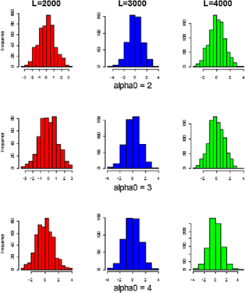
Figure 1: Distribution of normalized $(\widehat{\alpha}_{L}-\alpha_{0})$ by varying $L$ and $\alpha_{0}$, under Condition 4.

Table 2 provides the results for the classical Shapiro–Wilk Gaussianity test performed on simulations obtained by varying $\alpha_{0}$ and the number of multipoles $L$. Asymptotic Gaussianity is clearly supported.

Let us now focus on the more general Condition 3. Figure 2 represents the empirical distribution of $(L/4\sqrt{2}\log L)(\widehat{\alpha}_{L}-\alpha_{0})$ in case $\alpha_{0}=3$, $\kappa=1$ and the corresponding narrow-band estimates, whose results are summarized in Table 3. The improvement in the bias factor with the latter procedure is immediately evident.

Once more, asymptotic Gaussianity is strongly supported by the Shapiro–Wilk test, see again Table 3.

Considering the correction term $c_{L}$ from Remark 4, the sample bias is consistent with the asymptotic value to three decimal digits.

In Figure 3, we report the results obtained on a set of simulations under Condition 2, where we have:

$$G(l)=G_{0}\biggl{\{}1+\frac{1}{l}-\frac{1}{l^{2}}\biggr{\}}$$

with $G_{0}=2$, $\alpha_{0}=4$, $L=4000$, $L_{1}=3750$.

=280pt Sample frequencies $\alpha_{0}$ $L$ $-1.96$ $-1$ $-0.68$ $0$ $0.68$ $1$ $1.96$ 2 2000 4 19.2 29.2 48.6 22.8 14.2 4 3000 4.5 18.4 26.8 51 23.33 14.36 3.6 4000 4.4 17.7 25.2 49.1 23.43 13.87 4.8 3 2000 4.4 19.2 29.2 51.5 24.03 15.17 3.6 3000 4.3 18.4 26.8 48.9 23.2 13.43 3.8 4000 4.2 17.9 26.4 50.8 23.07 14.13 3.7 4 2000 4.4 21.6 30.2 50.9 22.73 14.94 5.5 3000 4.2 21.2 29.8 50.4 25.07 15.87 4.3 4000 4.2 17.9 27.1 50.4 22.7 13.73 4.2

Table 1: Quantiles of $L/4\sqrt{2}\log L(\widehat{\alpha}_{L}-\alpha_{0})$

=280pt Shapiro–Wilk test $\alpha_{0}$ $L$ $W$ $p$-value 2 2000 0.9976 0.685 3000 0.9978 0.667 4000 0.9983 0.373 3 2000 0.9976 0.691 3000 0.9980 0.842 4000 0.9985 0.945 4 2000 0.9987 0.670 3000 0.998 0.286 4000 0.9985 0.578

Table 2: Shapiro–Wilk test under Condition 4

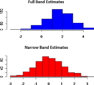
Figure 2: Comparison among biased and narrow estimates ($\kappa=1$, $L=2000$, $\alpha_{0}=3$), under Condition 3.

=280pt Shapiro–Wilk test $L$ $L_{1}$ Mean Var $W$ $p$-value 2000 1550 $0.072$ 0.959 0.9985 0.950 1700 $0.018$ 0.951 0.997 0.495 1850 $-0.016$ 1.004 0.9977 0.739 3000 2400 $0.092$ 1.130 0.9949 0.920 2600 $0.072$ 0.928 0.9951 0.745 2800 $-0.02$ 1.06 0.9965 0.340 4000 3250 $0.006$ 0.985 0.9968 0.443 3500 $0.004$ 1.097 0.998 0.834 3750 $0.0007$ 1.073 0.9982 0.874

Table 3: Normalized Narrow bands data, under Condition 3, $\kappa=1$, $\alpha_{0}=4$, $G_{0}=2$

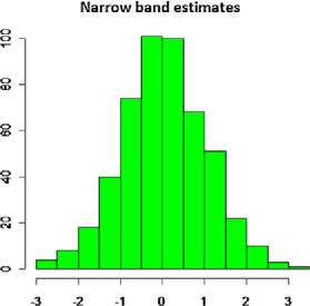
Figure 3: Distribution of normalized $(\widehat{\alpha}_{L}-\alpha_{0})$ under Condition 2.

We obtain a mean value $\mathbb{E}(\widehat{\alpha}_{L}-\alpha_{0})=0.040$ and a normalized variance of $0.9918$. Shapiro–Wilk Gaussianity test gives as result $W=0.9981$ with a $p$-$\mbox{value}=0.8669$. Table 4 compares sample variance, bias and mean squared errors obtained for simulations with different values of $L$, $\kappa$ and $\alpha_{0}$ with $N=5000$ iterations.

Table 4: Sample Variance, Bias and MSE of estimators $\widehat{\alpha}_{L}$ and $\widehat{\alpha}_{L_{1},L}$ for different values of $L=1000,2000,5000,10\,000$ and $\kappa=1,2$ ($\alpha_{0}=3$)

$\kappa$	Band	Var	Bias	MSE	Var	Bias	MSE
$L=1000$					$L=5000$
1	Full	$7.9\cdot 10^{-6}$	$0.004$	$2.4\cdot 10^{-5}$	$3.2\cdot 10^{-7}$	$0.0008$	$9.7\cdot 10^{-7}$
	Nar.	$1.4\cdot 10^{-4}$	$0.001$	$1.5\cdot 10^{-4}$	$5.4\cdot 10^{-5}$	$0.0003$	$5.4\cdot 10^{-5}$
2	Full	$8.0\cdot 10^{-6}$	$0.008$	$7.1\cdot 10^{-5}$	$3.3\cdot 10^{-7}$	$0.002$	$6.1\cdot 10^{-6}$
	Nar.	$1.4\cdot 10^{-4}$	$0.002$	$1.5\cdot 10^{-4}$	$5.3\cdot 10^{-5}$	$0.0006$	$5.4\cdot 10^{-5}$
$L=2000$					$L=10\,000$
1	Full	$1.9\cdot 10^{-6}$	0.002	$5.8\cdot 10^{-6}$	$8.1\cdot 10^{-8}$	0.0004	$2.4\cdot 10^{-7}$
	Nar.	$9.6\cdot 10^{-5}$	0.0005	$9.6\cdot 10^{-5}$	$1.3\cdot 10^{-5}$	$9\cdot 10^{-5}$	$1.3\cdot 10^{-5}$
2	Full	$1.9\cdot 10^{-6}$	0.004	$1.8\cdot 10^{-5}$	$8.1\cdot 10^{-8}$	0.0008	$2.4\cdot 10^{-7}$
	Nar.	$9.6\cdot 10^{-5}$	0.001	$9.6\cdot 10^{-5}$	$1.3\cdot 10^{-5}$	0.0002	$1.3\cdot 10^{-5}$

The simulations show that full-band estimators is characterized by a smaller MSE with respect to the corresponding narrow band estimators obtained on the same data sets, due to the smallest value of the variance. Hence, full band estimates seem to be more efficient than the narrow band ones, although they appear to be more robust. Note that for the sake of the brevity we report only the data concerning $\alpha_{0}=3$, because data obtained for $\alpha_{0}=2,4$ lead to very similar results.

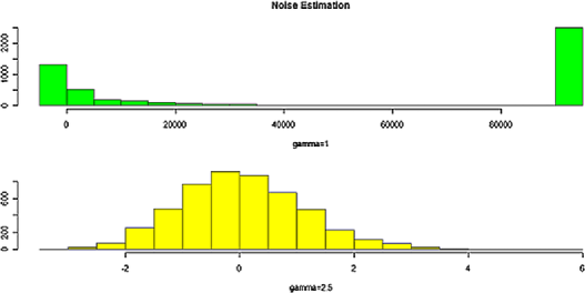
Figure 4: Distribution of normalized $\widetilde{\alpha}-\alpha_{0}$ ($\alpha_{0}=3$, $L=1000$) in presence of noise ($\gamma=1$ and $2.5$).

In Figure 4, we report results on simulations (iterated $N=5000$ times) which take in account also the presence of the noise, using $\alpha_{0}=3$, $L=1000$ and by varying the value of $\gamma$. In these simulations, we consider four cases. In the cases $\gamma=5$ and $\gamma=3$, the results obtained put in evidence that in the case $\gamma>\alpha_{0}$ the noise does not affect the signal detected (we omit these results in the figure). If instead $\gamma=2.5$, we obtain the convergence of the estimator to $\alpha_{0}$ with the rate of convergence as described in Theorem 4: in this case $\mathbb{E}(\widetilde{\alpha}_{L})=0.005$, while the variance of the normalized $\widetilde{\alpha}_{L}$ corresponds to 1.22. Shapiro–Wilk normality test provides $W=0.9919$ with $p$-$\mbox{value}=2.68\cdot 10^{-16}$. Finally, if $\gamma=1$ (and then $\gamma<\alpha_{0}-1$) the estimate computed assumes mainly values close to $\alpha_{\max}$, the highest value which is allowed by the computational point of view (in the figure $\alpha_{\max}=50$), hence it seems to diverge.

8 Conclusions

We view this paper as a first contribution in an area which deserves much further research, that is, the investigation of asymptotic properties for parametric estimators on a single realization of an isotropic random field on the sphere. As mentioned earlier, an enormous amount of applied papers have focussed on this issue, especially in a Cosmological framework, but no rigorous results seem currently available. Our results suggest that consistency and asymptotic Gaussianity are feasible for spectral index estimators, the rate of convergence being $L/\log L$; these estimates are centred on zero in “parametric” circumstances, that is, where the correct model being provided for $C_{l}$ up to a factor $\mathrm{o}(\frac{1}{l})$. When the latter assumption fails, alternatively, narrow-band estimates can be entertained; these estimates ensure convergence to a zero-mean Gaussian distribution, with a slightly slower convergence rate.

Many questions are left open by these results. The first we mention is the characterization of a whole class of parameters for which asymptotic Gaussianity and consistency may continue to hold. More challenging is the possibility to relax the Gaussian assumption and consider more general, finite-variance isotropic Gaussian fields. In this respect, results in [27] suggest that the Gaussianity assumption may indeed play a crucial role, as high-frequency consistency and Gaussianity seem very tightly related, for instance, when considering the asymptotic behavior of the angular power spectrum. It seems also important to explore the connection between the spherical estimates we have been considering and fixed-domain asymptotic results for Matern-type covariances, as discussed on $\mathbb{R}^{d}$ by [25, 1, 40, 41] and others. Likewise, the high-frequency behaviour of Bayesian estimates definitely deserves some investigation in this framework, especially considering the growing interest for Bayesian techniques in the astrophysical community.

For future work, we aim at relaxing some of the assumptions introduced in this paper to make these techniques more directly applicable on existing datasets. The harmonic estimates we have been focussing on require the observation of the random field on the full sphere. This condition often fails in practice: for instance, in a Cosmological framework large regions of the sky are not observable, because they are masked by Foreground sources such as the Milky Way. In ongoing research (see [10]), we are hence considering a Whittle-type estimator based on spherical wavelets (needlets, see [31, 29, 3]), rather than standard Fourier analysis. These estimates have, however, a larger asymptotic variance than the Fourier methods considered here; in a sense, this is an instance of the standard trade-off between robustness and efficiency. Thus, the material in the present paper presents a benchmark for optimal procedures under favourable experimental circumstances, and the right starting point for further developments under more challenging experimental set-ups.

Appendix

Consistency results

Proof of Theorem 1 To establish consistency, we shall resort to a technique developed by [7] and [37]. In particular, let us now write

$$\Delta R_{L}(\alpha,\alpha_{0}) = R_{L}(\alpha)-R_{L}(\alpha_{0})$$

$$= \log\frac{\widehat{G}(\alpha)}{G(\alpha)}-\log\frac{\widehat{G}(\alpha_{0})}{G(\alpha_{0})}-\frac{(\alpha-\alpha_{0})}{\sum_{l=1}^{L}(2l+1)}\sum_{l=1}^{L}(2l+1)\log l$$

$${}+\log\frac{G(\alpha)}{G(\alpha_{0})},$$

where

$$G(\alpha) = \frac{1}{\sum_{l=1}^{L}(2l+1)}\sum_{l=1}^{L}(2l+1)\frac{G_{0}l^{-\alpha_{0}}}{l^{-\alpha}},\qquad G(\alpha_{0})=G_{0},$$

$$\log\frac{G(\alpha)}{G(\alpha_{0})} = \log\Biggl{\{}\frac{1}{\sum_{l=1}^{L}(2l+1)}\sum_{l=1}^{L}(2l+1)l^{\alpha-\alpha_{0}}\Biggr{\}}$$

so that

$$\Delta R_{L}(\alpha,\alpha_{0}) = U_{L}(\alpha,\alpha_{0})-T_{L}(\alpha,\alpha_{0}),$$

$$U_{L}(\alpha,\alpha_{0}) = -\frac{(\alpha-\alpha_{0})}{\sum_{l=1}^{L}(2l+1)}\sum_{l=1}^{L}(2l+1)\log l+\log\frac{G(\alpha)}{G(\alpha_{0})},$$ (19)

$$T_{L}(\alpha,\alpha_{0}) = \log\frac{\widehat{G}(\alpha_{0})}{G(\alpha_{0})}-\log\frac{\widehat{G}(\alpha)}{G(\alpha)}.$$ (20)

The proof is then completed with the aid of the auxiliary Lemmas 6, 7 that we shall discuss below. Indeed

$$\Pr\bigl{\{}|\widehat{\alpha}_{L}-\alpha_{0}|>\varepsilon\bigr{\}} \leq \Pr\Bigl{\{}\inf_{|\alpha-\alpha_{0}|>\varepsilon}\Delta R_{L}(\alpha,\alpha_{0})\leq 0\Bigr{\}}$$

$$\leq \Pr\Bigl{\{}\inf_{|\alpha-\alpha_{0}|>\varepsilon}\bigl{[}U_{L}(\alpha,\alpha_{0})-T_{L}(\alpha,\alpha_{0})\bigr{]}\leq 0\Bigr{\}}.$$

For $\alpha_{0}-\alpha<2$ the previous probability is bounded by, for any $\delta>0$

$$\leq\Pr\Bigl{\{}\inf_{|\alpha-\alpha_{0}|>\varepsilon}U_{L}(\alpha,\alpha_{0})\leq\delta\Bigr{\}}+\Pr\Bigl{\{}\sup_{|\alpha-\alpha_{0}|>\varepsilon}T_{L}(a,\alpha_{0})>0\Bigr{\}}$$

and

$$\lim_{L\rightarrow\infty}\Pr\Bigl{\{}\sup_{|\alpha-\alpha_{0}|>\varepsilon}T_{L}(a,\alpha_{0})>0\Bigr{\}}=0$$

from Lemma 7, while from Lemma 6 there exist $\delta_{\varepsilon}=(1+\varepsilon/2)-\log(1+\varepsilon/2)-1>0$ such that

$$\lim_{L\rightarrow\infty}\Pr\Bigl{\{}\inf_{|\alpha-\alpha_{0}|>\varepsilon}U_{L}(\alpha,\alpha_{0})\leq\delta_{\varepsilon}\Bigr{\}}=0.$$

For $\alpha_{0}-\alpha=2$ or $\alpha_{0}-\alpha>2$ the same result is obtained by dividing $\Delta R_{L}(\alpha,\alpha_{0})$ by, respectively, $\log\log L$ or $\log L$ and then resorting again to Lemmas 6, 7.

Now note that

$$\widehat{G}(\widehat{\alpha}_{L})-G_{0} = \frac{1}{\sum_{l=1}^{L}(2l+1)}\sum_{l=1}^{L}(2l+1)\frac{\widehat{C}_{l}}{l^{-\widehat{\alpha}_{L}}}$$

$${}-\frac{1}{\sum_{l=1}^{L}(2l+1)}\sum_{l=1}^{L}(2l+1)\frac{G_{0}l^{-\alpha_{0}}}{l^{-\alpha_{0}}}$$

$$= \frac{1}{\sum_{l=1}^{L}(2l+1)}\sum_{l=1}^{L}(2l+1)G_{0}l^{-(\alpha_{0}-\widehat{\alpha}_{L})}\biggl{\{}\biggl{(}\frac{\widehat{C}_{l}}{G_{0}l^{-\alpha_{0}}}-1\biggr{)}+\bigl{(}1-l^{(\alpha_{0}-\widehat{\alpha}_{L})}\bigr{)}\biggr{\}}.$$

Clearly:

$$\bigl{|}\widehat{G}(\widehat{\alpha}_{L})-G_{0}\bigr{|} \leq \Biggl{|}\frac{1}{\sum_{l=1}^{L}(2l+1)}\sum_{l=1}^{L}(2l+1)G_{0}l^{-(\alpha_{0}-\widehat{\alpha}_{L})}\biggl{\{}\biggl{(}\frac{\widehat{C}_{l}}{G_{0}l^{-\alpha_{0}}}-1\biggr{)}\biggr{\}}\Biggr{|}$$

$${}+\Biggl{|}\frac{G_{0}}{\sum_{l=1}^{L}(2l+1)}\sum_{l=1}^{L}(2l+1)\bigl{(}l^{-(\alpha_{0}-\widehat{\alpha}_{L})}-1\bigr{)}\Biggr{|}$$

$$= |G_{A}|+|G_{B}|,$$

so that

$$\Pr\bigl{(}\bigl{|}\widehat{G}(\widehat{\alpha}_{L})-G_{0}\bigr{|}\geq\varepsilon\bigr{)}\leq\Pr\biggl{(}|G_{A}|\geq\frac{\varepsilon}{2}\biggr{)}+\Pr\biggl{(}|G_{B}|\geq\frac{\varepsilon}{2}\biggr{)}.$$

Observe that:

$$\Pr\biggl{\{}|G_{A}|\geq\frac{\varepsilon}{2}\biggr{\}} \leq \Pr\biggl{\{}\biggl{[}|G_{A}|\geq\frac{\varepsilon}{2}\biggr{]}\cap\biggl{[}|\alpha_{0}-\widehat{\alpha}_{L}|<\frac{1}{3}\biggr{]}\biggr{\}}$$

$${}+\Pr\biggl{\{}|\alpha_{0}-\widehat{\alpha}_{L}|\geq\frac{1}{3}\biggr{\}}$$

$$\leq \Pr\Biggl{\{}\Biggl{[}\frac{1}{\sum_{l=1}^{L}(2l+1)}\sum_{l=1}^{L}(2l+1)G_{0}l^{1/3}\biggl{|}\frac{\widehat{C}_{l}}{G_{0}l^{-\alpha_{0}}}-1\biggr{|}\geq\varepsilon\Biggr{]}\Biggr{\}}+\mathrm{o}_{L}(1)$$

$$\leq \frac{1}{\varepsilon}\frac{1}{\sum_{l=1}^{L}(2l+1)}\sum_{l=1}^{L}(2l+1)G_{0}l^{1/3}\mathbb{E}\biggl{|}\frac{\widehat{C}_{l}}{G_{0}l^{-\alpha_{0}}}-1\biggr{|}+\mathrm{o}_{L}(1)$$

$$\leq \frac{C}{\varepsilon}\frac{1}{\sum_{l=1}^{L}(2l+1)}\sum_{l=1}^{L}(2l+1)G_{0}l^{1/3}l^{-1/2}+\mathrm{o}_{L}(1)$$

$$= \frac{C}{\varepsilon}\frac{L^{11/6}}{\sum_{l=1}^{L}(2l+1)}+\mathrm{o}_{L}(1)=\mathrm{o}_{L}(1).$$

As far as the second term is concerned, we have, for a suitably small $\delta>0$:

$$\Pr\biggl{(}|G_{B}|\geq\frac{\varepsilon}{2}\biggr{)} = \Pr\biggl{(}\biggl{[}|G_{B}|\geq\frac{\varepsilon}{2}\biggr{]}\cap\bigl{[}\log l(\alpha_{0}-\widehat{\alpha}_{L})\bigr{]}<\delta\biggr{)}$$

$${}+\Pr\bigl{(}\log l(\alpha_{0}-\widehat{\alpha}_{L})\geq\delta\bigr{)}$$

$$= \Pr\biggl{(}\biggl{[}|G_{B}|\geq\frac{\varepsilon}{2}\biggr{]}\cap\bigl{[}\log l(\alpha_{0}-\widehat{\alpha}_{L})\bigr{]}<\delta\biggr{)}+\mathrm{o}_{L}(1)$$

and using $|\mathrm{e}^{-x}-1|\leq x$ for $0\leq x\leq 1$, we obtain

$$\bigl{|}l^{-(\alpha_{0}-\widehat{\alpha}_{L})}-1\bigr{|} = \bigl{|}\exp\bigl{(}-\log l(\alpha_{0}-\widehat{\alpha}_{L})\bigr{)}-1\bigr{|}\leq\log l|\alpha_{0}-\widehat{\alpha}_{L}|,$$

$$\Pr\biggl{(}\biggl{[}|G_{B}|\geq\frac{\varepsilon}{2}\biggr{]}\cap\bigl{[}\log l(\alpha_{0}-\widehat{\alpha}_{L})\bigr{]}<\delta\biggr{)}$$

$$\quad\leq\Pr\Biggl{(}\frac{G_{0}}{\sum_{l=1}^{L}(2l+1)}\sum_{l=1}^{L}(2l+1)\bigl{|}\bigl{(}l^{-(\alpha_{0}-\widehat{\alpha}_{L})}-1\bigr{)}\bigr{|}\geq\frac{\varepsilon}{2}\cap\bigl{[}\log l(\alpha_{0}-\widehat{\alpha}_{L})\bigr{]}<\delta\Biggr{)}$$

$$\quad\leq\frac{1}{\varepsilon}\mathbb{E}\Biggl{\{}\frac{G_{0}}{\sum_{l=1}^{L}(2l+1)}\sum_{l=1}^{L}(2l+1)\log l|\alpha_{0}-\widehat{\alpha}_{L}|\Biggr{\}}$$

$$\quad\leq\frac{C}{\varepsilon}\frac{G_{0}}{\sum_{l=1}^{L}(2l+1)}\sum_{l=1}^{L}(2l+1)\log l\frac{\log L}{L}=\mathrm{o}_{L}(1),$$

where we have used

$$\mathbb{E}|\alpha_{0}-\widehat{\alpha}_{L}|\leq\bigl{\{}\mathbb{E}|\alpha_{0}-\widehat{\alpha}_{L}|^{2}\bigr{\}}^{1/2}=\mathrm{O}\biggl{(}\frac{\log L}{L}\biggr{)},$$

which under Condition 2 will be established in the proof of Theorem 2.

The first auxiliary result we shall need concerns $G,\widehat{G}$ and their $k$th order derivatives $G_{k},\widehat{G}_{k}$, that is,

$$\widehat{G}_{k}(\alpha) = \frac{1}{\sum_{l=1}^{L}(2l+1)}\sum_{l=1}^{L}(2l+1)\bigl{(}\log^{k}l\bigr{)}\frac{\widehat{C}_{l}}{l^{-\alpha}},\qquad k=0,1,2,\ldots,$$

$$G_{k}(\alpha) = \frac{1}{\sum_{l=1}^{L}(2l+1)}\sum_{l=1}^{L}(2l+1)\bigl{(}\log^{k}l\bigr{)}\frac{G_{0}l^{-\alpha_{0}}}{l^{-\alpha}},\qquad k=0,1,2,\ldots,$$

where $\widehat{G}_{0}(\alpha)=\widehat{G}(\alpha)$ and $G_{0}(\alpha)=G(\alpha)$ defined as above.

Lemma 5.

Under Condition 2, for all $2>\alpha_{0}-\alpha>\varepsilon>0$, as $L\rightarrow\infty$, we have

$$\sup_{\alpha}\biggl{|}\log\frac{\widehat{G}_{k}(\alpha)}{G_{k}(\alpha)}\biggr{|}=\mathrm{o}_{p}(1).$$

On the other hand, if $\alpha_{0}-\alpha\geq 2$,

$$\sup_{\alpha}\biggl{|}\log\frac{\widehat{G}_{k}(\alpha)}{G_{k}(\alpha)}\biggr{|}=\mathrm{O}_{p}(1).$$

Proof.

Let us first focus on the case where $\alpha-\alpha_{0}>-2$. For clarity of exposition, we start from a simplified parametric version of Condition 1, that is, we assume that we have exactly

$$C_{l}(\vartheta)=C_{l}(G_{0},\alpha_{0})=G_{0}l^{-\alpha_{0}}.$$

Let us write first

$$\frac{\widehat{G}_{k}(\alpha)}{G_{k}(\alpha)}-1 = \frac{(\sum_{l=1}^{L}(2l+1)(\log l)^{k}{\widehat{C}_{l}}/{l^{-\alpha}})/({\sum_{l=1}^{L}(2l+1)})}{(\sum_{l=1}^{L}(2l+1)(\log l)^{k}{G_{0}l^{-\alpha_{0}}}/{l^{-\alpha}})/({\sum_{l=1}^{L}(2l+1)})}-1$$

$$= \frac{\sum_{l=1}^{L}(2l+1)(\log l)^{k}G_{0}l^{\alpha-\alpha_{0}}\{{\widehat{C}_{l}}/({G_{0}l^{-\alpha_{0}}})-1\}}{\sum_{l=1}^{L}(2l+1)(\log l)^{k}G_{0}l^{\alpha-\alpha_{0}}}.$$

Fixed $0<\beta<\frac{1}{2}$, we have, for all $l$:

$$\Pr\biggl{(}\biggl{|}\frac{\sum_{l=1}^{L}(2l+1)G_{0}l^{\alpha-\alpha_{0}}(\log l)^{k}\{{\widehat{C}_{l}}/({G_{0}l^{-\alpha_{0}}})-1\}}{\sum_{l=1}^{L}(2l+1)(\log l)^{k}G_{0}l^{\alpha-\alpha_{0}}}\biggr{|}>\delta_{\varepsilon}\biggr{)}$$

$$\quad\leq\Pr\biggl{(}L^{\beta}\biggl{|}\frac{\sum_{l=1}^{L}\sqrt{(2l+1)}(\log l)^{k}l^{\alpha-\alpha_{0}}}{\sum_{l=1}^{L}(2l+1)(\log l)^{k}l^{\alpha-\alpha_{0}}}\biggr{|}\frac{\sup_{l}\sqrt{(2l+1)}|{\widehat{C}_{l}}/({G_{0}l^{-\alpha_{0}}})-1|}{L^{\beta}}>\delta_{\varepsilon}\biggr{)}$$

$$\quad\leq\Pr\biggl{(}\sup_{l}\sqrt{(2l+1)}\biggl{|}\frac{\widehat{C}_{l}}{G_{0}l^{-\alpha_{0}}}-1\biggr{|}>\delta_{\varepsilon}L^{\beta}\biggr{)},$$

because

$$L^{\beta}\frac{\sum_{l=1}^{L}\sqrt{(2l+1)}(\log l)^{k}l^{\alpha-\alpha_{0}}}{\sum_{l=1}^{L}(2l+1)(\log l)^{k}l^{\alpha-\alpha_{0}}}=C\frac{L^{\beta+{3}/{2}+\alpha-\alpha_{0}}\log^{k}L}{L^{2+\alpha-\alpha_{0}}\log^{k}L}=CL^{\beta-1/2}=\mathrm{o}(1).$$

Now

$$\Pr\biggl{\{}\sup_{l}\sqrt{(2l+1)}\biggl{|}\frac{\widehat{C}_{l}}{G_{0}l^{-\alpha_{0}}}-1\biggr{|}>\delta_{\varepsilon}L^{\beta}\biggr{\}}$$

$$\quad\leq L\max_{l}\Pr\biggl{\{}\sqrt{(2l+1)}\biggl{|}\frac{\widehat{C}_{l}}{G_{0}l^{-\alpha_{0}}}-1\biggr{|}>\delta_{\varepsilon}L^{\beta}\biggr{\}}$$

and

$$\Pr\biggl{\{}\sqrt{(2l+1)}\biggl{|}\frac{\widehat{C}_{l}}{G_{0}l^{-\alpha_{0}}}-1\biggr{|}>\delta_{\varepsilon}L^{\beta}\biggr{\}}\leq C\frac{\mathbb{E}[\sqrt{(2l+1)}|{\widehat{C}_{l}}/({G_{0}l^{-\alpha_{0}}})-1|]^{M}}{\delta_{\varepsilon}^{M}L^{M\beta}}=\mathrm{O}\bigl{(}L^{-M\beta}\bigr{)},$$

uniformly in $l$, see, for instance, [28], such that $M>1/\beta$. Hence,

$$\Pr\biggl{\{}\sup_{l}\sqrt{(2l+1)}\biggl{|}\frac{\widehat{C}_{l}}{G_{0}l^{-\alpha_{0}}}-1\biggr{|}>\delta_{\varepsilon}L^{\beta}\biggr{\}}=\mathrm{O}\bigl{(}L^{1-M\beta}\bigr{)}=\mathrm{o}_{L}(1).$$

For the general semiparametric case, the only difference is to be found in the expressions for $\mathbb{E}\widehat{C}_{l}$, which under Condition 2 becomes

$$\mathbb{E}\widehat{C}_{l}=G_{0}l^{-\alpha_{0}}\bigl{(}1+\mathrm{O}\bigl{(}l^{-1}\bigr{)}\bigr{)},$$

where the bound $\mathrm{O}(l^{-1})$ is uniform over $\alpha$ by assumption. As before, we hence obtain

$$\frac{\widehat{G}_{k}(\alpha)}{G_{k}(\alpha)}-1$$

$$\quad=\frac{\sum_{l=1}^{L}(2l+1)(\log l)^{k}{\widehat{C}_{l}}/{l^{-\alpha}}-\sum_{l=1}^{L}(2l+1)(\log l)^{k}{G_{0}l^{-\alpha_{0}}}/{l^{-\alpha}}}{\sum_{l=1}^{L}(2l+1)(\log l)^{k}{G_{0}l^{-\alpha_{0}}}/{l^{-\alpha}}}$$

$$\quad=\frac{\sum_{l=1}^{L}(2l+1)(\log l)^{k}G_{0}l^{\alpha-\alpha_{0}}\{{\widehat{C}_{l}}/({G_{0}l^{-\alpha_{0}}})-{\mathbb{E}\widehat{C}_{l}}/({G_{0}l^{-\alpha_{0}}})\}}{\sum_{l=1}^{L}(2l+1)(\log l)^{k}G_{0}l^{\alpha-\alpha_{0}}}$$

$$\qquad{}+\frac{\sum_{l=1}^{L}(2l+1)(\log l)^{k}G_{0}l^{\alpha-\alpha_{0}}\{\mathrm{O}({1}/{l})\}}{\sum_{l=1}^{L}(2l+1)(\log l)^{k}G_{0}l^{\alpha-\alpha_{0}}}.$$

The second summand is immediately observed to be $\mathrm{O}(\frac{1}{L})$. By the same argument as before, for $0<\beta<\frac{1}{2}$, we have, for all $l$:

$$\Pr\biggl{\{}\biggl{|}\frac{\sum_{l=1}^{L}(2l+1)(\log l)^{k}G_{0}l^{\alpha-\alpha_{0}}\{{\widehat{C}_{l}}/({G_{0}l^{-\alpha_{0}}})-{\mathbb{E}\widehat{C}_{l}}/({G_{0}l^{-\alpha_{0}}})\}}{\sum_{l=1}^{L}(2l+1)(\log l)^{k}G_{0}l^{\alpha-\alpha_{0}}}\biggr{|}>\delta_{\varepsilon}\biggr{\}}$$

$$\quad\leq\Pr\biggl{\{}\sup_{l}\sqrt{(2l+1)}\frac{\mathbb{E}\widehat{C}_{l}}{G_{0}l^{-\alpha_{0}}}\biggl{|}\frac{\widehat{C}_{l}}{\mathbb{E}\widehat{C}_{l}}-1\biggr{|}>\delta_{\varepsilon}L^{\beta}\biggr{\}}$$

$$\quad\leq\Pr\biggl{\{}\sup_{l}\sqrt{(2l+1)}\biggl{\{}1+\mathrm{O}\biggl{(}\frac{1}{l}\biggr{)}\biggr{\}}\biggl{|}\frac{\widehat{C}_{l}}{\mathbb{E}\widehat{C}_{l}}-1\biggr{|}>\delta_{\varepsilon}L^{\beta}\biggr{\}}.$$

The rest of the proof is analogous to the argument we provided before, and hence omitted.

For the case where $\alpha_{0}-\alpha\geq 2$, it suffices to note that

$$\frac{\widehat{G}_{k}(\alpha)}{G_{k}(\alpha)}=\frac{(\sum_{l=1}^{L}(2l+1)(\log l)^{k}{\widehat{C}_{l}}/{l^{-\alpha}})/({\sum_{l=1}^{L}(2l+1)})}{(\sum_{l=1}^{L}(2l+1)(\log l)^{k}{G_{0}l^{-\alpha_{0}}}/{l^{-\alpha}})/({\sum_{l=1}^{L}(2l+1)})}>0\qquad\mbox{with probability 1}$$

and

$$\mathbb{E}\frac{\widehat{G}_{k}(\alpha)}{G_{k}(\alpha)}=\frac{(\sum_{l=1}^{L}(2l+1)(\log l)^{k}({G_{0}l^{-\alpha_{0}}}/{l^{-\alpha}})\{1+\mathrm{O}({1}/{l})\})/({\sum_{l=1}^{L}(2l+1)})}{(\sum_{l=1}^{L}(2l+1)(\log l)^{k}{G_{0}l^{-\alpha_{0}}}/{l^{-\alpha}})/({\sum_{l=1}^{L}(2l+1)})}=\mathrm{O}(1).\quad$$

∎

We are now in the position to establish the asymptotic behavior of $U_{L}(\alpha,\alpha_{0})$ in (19), for which we have the following:

Lemma 6.

For all $2>\alpha_{0}-\alpha>\varepsilon>0$, we have that

$$\lim_{L\rightarrow\infty}\Biggl{\{}-\frac{(\alpha-\alpha_{0})}{\sum_{l=1}^{L}(2l+1)}\sum_{l=1}^{L}(2l+1)\log l+\log\frac{G(\alpha)}{G(\alpha_{0})}\Biggr{\}}$$

$$\quad=\lim_{L\rightarrow\infty}\Biggl{[}\log\Biggl{\{}\frac{1}{\sum_{l=1}^{L}(2l+1)}\sum_{l=1}^{L}(2l+1)l^{\alpha-\alpha_{0}}\Biggr{\}}-\frac{(\alpha-\alpha_{0})}{\sum_{l=1}^{L}(2l+1)}\sum_{l=1}^{L}(2l+1)\log l\Biggr{]}$$

$$\quad=\bigl{(}1+(\alpha-\alpha_{0})/2\bigr{)}-\log\bigl{(}1+(\alpha-\alpha_{0})/2\bigr{)}-1>\delta_{\varepsilon}>0.$$

Moreover, if $\alpha_{0}-\alpha=2$,

$$\lim_{L\rightarrow\infty}\frac{1}{\log\log L}\Biggl{\{}-\frac{(\alpha-\alpha_{0})}{\sum_{l=1}^{L}(2l+1)}\sum_{l=1}^{L}(2l+1)\log l+\log\frac{G(\alpha)}{G(\alpha_{0})}\Biggr{\}}=1>0$$

and for $\alpha_{0}-\alpha>2$,

$$\lim_{L\rightarrow\infty}\frac{1}{\log L}\Biggl{\{}-\frac{(\alpha-\alpha_{0})}{\sum_{l=1}^{L}(2l+1)}\sum_{l=1}^{L}(2l+1)\log l+\log\frac{G(\alpha)}{G(\alpha_{0})}\Biggr{\}}$$

$$\quad=\alpha_{0}-\alpha-2>0.$$

Proof.

Consider first the case $\alpha-\alpha_{0}>-2$

$$\log\Biggl{\{}\frac{1}{\sum_{l=1}^{L}(2l+1)}\sum_{l=1}^{L}(2l+1)l^{\alpha-\alpha_{0}}\Biggr{\}}$$

$$\quad=\log\Biggl{\{}\frac{(1+(\alpha-\alpha_{0})/2)}{L^{\alpha-\alpha_{0}}\sum_{l=1}^{L}(2l+1)}\sum_{l=1}^{L}(2l+1)l^{\alpha-\alpha_{0}}\Biggr{\}}$$

$$\qquad{}-\log\bigl{(}1+(\alpha-\alpha_{0})/2\bigr{)}+(\alpha-\alpha_{0})\log L,$$

where

$$\frac{(1+(\alpha-\alpha_{0})/2)}{L^{\alpha-\alpha_{0}}\sum_{l=1}^{L}(2l+1)}\sum_{l=1}^{L}(2l+1)l^{\alpha-\alpha_{0}}-1 = \mathrm{o}_{L}(1),$$

whence

$$\log\Biggl{\{}\frac{(1+(\alpha-\alpha_{0})/2)}{L^{\alpha-\alpha_{0}}\sum_{l=1}^{L}(2l+1)}\sum_{l=1}^{L}(2l+1)l^{\alpha-\alpha_{0}}\Biggr{\}} = \mathrm{o}_{L}(1).$$

Thus,

$$\log\Biggl{\{}\frac{1}{\sum_{l=1}^{L}(2l+1)}\sum_{l=1}^{L}(2l+1)l^{\alpha-\alpha_{0}}\Biggr{\}}-\frac{(\alpha-\alpha_{0})}{\sum_{l=1}^{L}(2l+1)}\sum_{l=1}^{L}(2l+1)\log l$$

$$\quad=-\log\bigl{(}1+(\alpha-\alpha_{0})/2\bigr{)}+(\alpha-\alpha_{0})\log L$$

$$\qquad{}-\frac{(\alpha-\alpha_{0})}{\sum_{l=1}^{L}(2l+1)}\sum_{l=1}^{L}(2l+1)\log l+\mathrm{o}_{L}(1)$$

$$\quad=\frac{(\alpha-\alpha_{0})}{\sum_{l=1}^{L}(2l+1)}\sum_{l=1}^{L}(2l+1)(\log L-\log l)$$

$$\qquad{}-\frac{(\alpha-\alpha_{0})}{2}+\frac{(\alpha-\alpha_{0})}{2}-\log\bigl{(}1+(\alpha-\alpha_{0})/2\bigr{)}+\mathrm{o}_{L}(1).$$

Now

$$\frac{(\alpha-\alpha_{0})}{\sum_{l=1}^{L}(2l+1)}\sum_{l=1}^{L}(2l+1)(\log L-\log l)-\frac{(\alpha-\alpha_{0})}{2}$$

$$\quad=-2(\alpha-\alpha_{0})\int_{0}^{1}x\log x\,\mathrm{d}x-\frac{(\alpha-\alpha_{0})}{2}+\mathrm{o}_{L}(1)=\mathrm{o}_{L}(1),$$

because

$$\int_{0}^{1}x\log x\,\mathrm{d}x=\biggl{[}\frac{x^{2}}{2}\log x\biggr{]}_{0}^{1}-\int_{0}^{1}\frac{x^{2}}{2}\frac{1}{x}\,\mathrm{d}x=-\frac{1}{4}.$$

We have hence proved that

$$\log\Biggl{\{}\frac{1}{\sum_{l=1}^{L}(2l+1)}\sum_{l=1}^{L}(2l+1)l^{\alpha-\alpha_{0}}\Biggr{\}}-\frac{(\alpha-\alpha_{0})}{\sum_{l=1}^{L}(2l+1)}\sum_{l=1}^{L}(2l+1)\log l$$

$$\quad=\bigl{(}1+(\alpha-\alpha_{0})/2\bigr{)}-\log\bigl{(}1+(\alpha-\alpha_{0})/2\bigr{)}-1+\mathrm{o}_{L}(1)>0$$

for all $|\alpha-\alpha_{0}|>\varepsilon$, $\alpha-\alpha_{0}>-2$.

Consider now the case $\alpha_{0}-\alpha\geq 2$. We can rewrite:

$$-\frac{(\alpha-\alpha_{0})}{\sum_{l=1}^{L}(2l+1)}\sum_{l=1}^{L}(2l+1)\log l+\log\frac{G(\alpha)}{G(\alpha_{0})}$$

$$\quad=\log\Biggl{\{}\frac{1}{\sum_{l=1}^{L}(2l+1)}\sum_{l=1}^{L}(2l+1)l^{\alpha-\alpha_{0}}\Biggr{\}}-\frac{(\alpha-\alpha_{0})}{\sum_{l=1}^{L}(2l+1)}\sum_{l=1}^{L}(2l+1)\log l$$

$$\quad=(\alpha_{0}-\alpha)\log L\Biggl{[}\frac{\log\sum_{l=1}^{L}(2l+1)l^{-(\alpha_{0}-\alpha)}}{(\alpha_{0}-\alpha)\log L}-\frac{\log\sum_{l=1}^{L}(2l+1)}{(\alpha_{0}-\alpha)\log L}$$

$$\qquad\hskip 64.0pt{}+\frac{1}{\sum_{l=1}^{L}(2l+1)}\sum_{l=1}^{L}(2l+1)\frac{\log l}{\log L}\Biggr{]}$$

$$\quad=(\alpha_{0}-\alpha)\log L[A_{L}+B_{L}+C_{L}].$$

For the term $A_{L}$:

$$\sum_{l=1}^{L}(2l+1)l^{-(\alpha_{0}-\alpha)}=c\sum_{l=1}^{L}l^{1-(\alpha_{0}-\alpha)}+\mathrm{o}_{L^{2-(\alpha_{0}-\alpha)}}(1)\rightarrow_{L}c>1,$$

because $\sum_{l=1}^{L}l^{1-(\alpha_{0}-\alpha)}$ is a convergent series when the exponent $1-(\alpha_{0}-\alpha)<-1;$ for $1-(\alpha_{0}-\alpha)=-1$, we have $\{\sum_{l=1}^{L}l^{1-(\alpha_{0}-\alpha)}/\log L\}\rightarrow 1$ and the argument is analogous. Therefore,

$$(\alpha_{0}-\alpha)\log L\times[A_{L}]=\cases{\mathrm{O}(\log\log L),&\quad for $\alpha_{0}-\alpha=2$,\cr\mathrm{O}(1),&\quad for $\alpha_{0}-\alpha>2$.}$$

As far as $B_{L}$ is concerned, we have $\log\sum_{l=1}^{L}(2l+1)=2\log L+\mathrm{o}(\log L)$, so that:

$$\lim_{L\rightarrow\infty}B_{L}=-\frac{2}{(\alpha_{0}-\alpha)};$$

finally, simple manipulations and standard properties of the logarithm (which is a slowly varying function, compare [6]) yield

$$\lim_{L\rightarrow\infty}C_{L}=\lim_{L\rightarrow\infty}\Biggl{[}\frac{1}{\sum_{l=1}^{L}(2l+1)}\sum_{l=1}^{L}(2l+1)\frac{\log l}{\log L}\Biggr{]}=1.$$

Summing up, we obtain:

$$\lim_{L\rightarrow\infty}\bigl{\{}(\alpha_{0}-\alpha)\log L[B_{L}+C_{L}]\bigr{\}}=\cases{0,&\quad for $\alpha_{0}-\alpha=2$,\cr(\alpha_{0}-\alpha)-2>0,&\quad for $\alpha_{0}-\alpha>2$,}$$

and the claimed result follows. ∎

In [37] a related computation was given for approximate Whittle estimates on stationary long memory processes in dimension $d=1$, that is, the limiting lower bound turned out to be $(1+(\alpha-\alpha_{0}))-\log(1+(\alpha-\alpha_{0}))-1+\mathrm{o}_{L}(1)>\delta_{\varepsilon}$. In view of this, we conjecture that for general $d$-dimensional spheres the lower bound will take the form

$$\biggl{(}1+\frac{(\alpha-\alpha_{0})}{d}\biggr{)}-\log\biggl{(}1+\frac{(\alpha-\alpha_{0})}{d}\biggr{)}-1+\mathrm{o}_{L}(1)>\delta_{\varepsilon}.$$

Now we look at $T_{L}(\alpha,\alpha_{0})$, for which we provide the following lemma.

Lemma 7.

Let $T_{L}(\alpha,\alpha_{0})$ defined as in (20). Under Condition 2, as $L\rightarrow\infty,$ we have

$$\sup_{\alpha}\bigl{|}T_{L}(\alpha,\alpha_{0})\bigr{|} = \mathrm{o}_{p}(1)\qquad\mbox{for }\alpha_{0}-\alpha<2,$$

$$\sup_{\alpha}\bigl{|}T_{L}(\alpha,\alpha_{0})\bigr{|} = \mathrm{O}_{p}(1)\qquad\mbox{for }\alpha_{0}-\alpha\geq 2.$$

Proof.

For $\alpha_{0}-\alpha<2$, consider first

$$\frac{\widehat{G}(\alpha_{0})}{G(\alpha_{0})}-1=\frac{1}{\sum_{l=1}^{L}(2l+1)}\sum_{l=1}^{L}(2l+1)\biggl{(}\frac{\widehat{C}_{l}}{G_{0}l^{-\alpha_{0}}}-1\biggr{)},$$

where we have easily, as $L\rightarrow\infty$,

$$\mathbb{E}\biggl{\{}\frac{\widehat{G}(\alpha_{0})}{G(\alpha_{0})}-1\biggr{\}} = \frac{1}{\sum_{l=1}^{L}(2l+1)}\sum_{l=1}^{L}(2l+1)\biggl{(}\frac{G_{0}l^{-\alpha_{0}}\{1+\mathrm{O}(l^{-1})\}}{G_{0}l^{-\alpha_{0}}}-1\biggr{)}\rightarrow 0,$$

$$\operatorname{Var}\biggl{\{}\frac{\widehat{G}(\alpha_{0})}{G(\alpha_{0})}\biggr{\}} = \biggl{\{}\frac{1}{\sum_{l=1}^{L}(2l+1)}\biggr{\}}^{2}\sum_{l=1}^{L}(2l+1)^{2}=\mathrm{O}\biggl{(}\frac{1}{L}\biggr{)},$$

whence by Slutzky’s lemma

$$\biggl{\{}\frac{\widehat{G}_{L}(\alpha_{0})}{G_{L}(\alpha_{0})}\stackrel{{\scriptstyle\mathbb{P}}}{{\longrightarrow}}1\biggr{\}}\Rightarrow\biggl{\{}\log\frac{\widehat{G}(\alpha_{0})}{G(\alpha_{0})}\stackrel{{\scriptstyle\mathbb{P}}}{{\longrightarrow}}0\biggr{\}}.$$

On the other hand, in view of Lemma 5, we have that:

$$\sup_{\alpha}\biggl{|}\log\frac{\widehat{G}(\alpha)}{G(\alpha)}\biggr{|}=\mathrm{o}_{p}(1),$$

whence the result follows easily. The proof for $\alpha_{0}-\alpha\geq 2$ is immediate. ∎

Some integral approximation results

The following lemma is straightforward.

Lemma 8.

Let $L_{1}<L$, then we have

$$\int_{L_{1}}^{L}2x^{1+s}\,\mathrm{d}x = \frac{1}{(1+{s}/{2})}\bigl{(}L^{2(1+{s}/{2})}-L_{1}^{2(1+{s}/{2})}\bigr{)};$$ (21)

$$\int_{L_{1}}^{L}2x^{1+s}\log x\,\mathrm{d}x = -\frac{L^{2(1+{s}/{2})}-L_{1}^{2(1+{s}/{2})}}{2(1+{s}/{2})^{2}}+\frac{L^{2(1+{s}/{2})}\log L-L_{1}^{2(1+{s}/{2})}\log L_{1}}{(1+{s}/{2})};$$

$$\int_{L_{1}}^{L}2x^{1+s}\log^{2}x\,\mathrm{d}x = \frac{L^{2(1+{s}/{2})}-L_{1}^{2(1+{s}/{2})}}{2(1+{s}/{2})^{3}}-\frac{L^{2(1+{s}/{2})}\log L-L_{1}^{2(1+{s}/{2})}\log L_{1}}{(1+{s}/{2})^{2}}$$

$${}+\frac{L^{2(1+{s}/{2})}\log^{2}L-L_{1}^{2(1+{s}/{2})}\log^{2}L_{1}}{(1+{s}/{2})}.$$

The next result is more delicate; for the sake of brevity, we prove only (24); (22) can be viewed as a simpler special case with $L_{1}=1$.

Proposition 9.

Let

$$Z_{L}(s):=\Biggl{[}\sum_{l=1}^{L}(2l+1)l^{1+s}\sum_{l=1}^{L}(2l+1)l^{1+s}(\log l)^{2}-\Biggl{(}\sum_{l=1}^{L}(2l+1)l^{1+s}\log l\Biggr{)}^{2}\Biggr{]}.$$

Then, for $s\in\mathbb{R}$:

$$\lim_{L\rightarrow\infty}\frac{1}{L^{4+2s}}Z_{L}(s)=\frac{1}{4(1+{s}/{2})^{4}}.$$ (22)

Moreover, let $L_{1}=1+L\cdot(1-g(L))$, where $0<g(L)<1$ is such that $\lim_{L\rightarrow\infty}g(L)=0$. If

$$Z_{L;g(L)}(s) = \sum_{l=L_{1}}^{L}(2l+1)l^{1+s}\sum_{l=L_{1}}^{L}(2l+1)l^{1+s}\bigl{(}\log^{2}l\bigr{)}$$

$${}-\Biggl{(}\sum_{l=L_{1}}^{L}(2l+1)l^{1+s}\log l\Biggr{)}^{2},$$

we have

$$\lim_{L\rightarrow\infty}\frac{1}{L^{4(1+{s}/{2})}g^{4}(L)}Z_{L;g(L)}(s)=K(s),$$ (24)

where

$$K(s)=\frac{1}{(1+{s}/{2})^{2}}\biggl{(}\frac{1}{12}s^{2}-\frac{1}{8}s+\frac{1}{3}\biggr{)}.$$

Note that for $s=0$,

$$K_{0}=K(s)|_{s=0}={\textstyle\frac{1}{3}}.$$ (25)

Proof of Proposition 9 We start by observing that

$$\Biggl{(}\sum_{l=L_{1}}^{L}(2l+1)l^{s}\log^{2}l\Biggr{)}\Biggl{(}\sum_{l=L_{1}}^{L}(2l+1)l^{s}\Biggr{)}$$

$$\quad=\frac{(L^{2(1+{s}/{2})}-L_{1}^{2(1+{s}/{2})})^{2}}{(1+{s}/{2})^{2}}\biggl{(}\frac{1}{2(1+{s}/{2})^{2}}+\frac{\log L}{(1+{s/2})}+\log^{2}L\biggr{)}$$

$$\qquad{}+\frac{(L^{2(1+{s}/{2})}-L_{1}^{2(1+{s}/{2})})L_{1}^{2(1+{s}/{2})}}{(1+{s/2})^{3}}\log\bigl{(}1-g(L)\bigr{)}$$

$$\qquad\hskip 11.0pt{}\times\biggl{(}\frac{1}{(1+{s/2})}-2\log L-\log^{2}\bigl{(}1-g(L)\bigr{)}\biggr{)}+\mathrm{o}_{L}(1);$$

$$\Biggl{(}\sum_{l=L_{1}}^{L}(2l+1)l^{s}\log l\Biggr{)}^{2}$$

$$\quad=\frac{(L^{2(1+{s}/{2})}-L_{1}^{2(1+{s}/{2})})^{2}}{(1+{s/2})^{2}}\biggl{(}\frac{1}{4(1+{s/2})^{2}}-\frac{\log L}{(1+{s/2})}+\log^{2}L\biggr{)}$$

$$\qquad{}+\frac{(L^{2(1+{s}/{2})}-L_{1}^{2(1+{s}/{2})})}{(1+{s/2})^{2}}L_{1}^{2(1+{s}/{2})}\log\bigl{(}1-g(L)\bigr{)}\biggl{(}\frac{1}{(1+{s/2})}-2\log L\biggr{)}$$

$$\qquad{}+\frac{L_{1}^{4(1+{s}/{2})}\log^{2}(1-g(L))}{(1+{s/2})^{2}}+\mathrm{o}_{L}(1),$$

so we obtain

$$Z_{L,g(L)}(s) = \frac{(L^{2(1+{s}/{2})}-L_{1}^{2(1+{s}/{2})})^{2}}{4(1+{s/2})^{4}}$$

$${}-\frac{L^{2(1+{s}/{2})}L_{1}^{2(1+{s}/{2})}\log^{2}(1-g(L))}{(1+{s/2})^{2}}+\mathrm{o}_{L}(1)$$

$$= \frac{L^{4(1+{s}/{2})}((1-(1-g(L))^{2(1+{s}/{2})}))^{2}}{4(1+{s/2})^{4}}$$

$${}-\frac{L^{4(1+{s}/{2})}(1-g(L))^{2(1+{s}/{2})}\log^{2}(1-g(L))}{(1+{s/2})^{2}}+\mathrm{o}_{L}(1).$$

Observe that

$$\log^{2}\bigl{(}1-g(L)\bigr{)} = \bigl{(}-g(L)-{\textstyle\frac{1}{2}}g^{2}(L)-{\textstyle\frac{1}{3}}g^{3}(L)+\mathrm{O}\bigl{(}g^{4}(L)\bigr{)}\bigr{)}^{2}$$

$$= g^{2}(L)+g^{3}(L)+\bigl{(}{\textstyle\frac{11}{12}}\bigr{)}g^{4}(L)+\mathrm{o}\bigl{(}g^{4}(L)\bigr{)},$$

while

$$\frac{(1-g(L))^{2(1+{s}/{2})}}{(1+{s/2})} = \frac{1}{(1+{s/2})}-2g(L)+\biggl{(}2\biggl{(}1+\frac{s}{2}\biggr{)}-1\biggr{)}g^{2}(L)$$

$${}-\frac{(2(1+{s/2})-1)(2(1+{s/2})-2)}{3}g^{3}(L)+\mathrm{o}\bigl{(}g^{3}(L)\bigr{)}.$$

Thus

$$\frac{L^{4(1+{s}/{2})}((1-(1-g(L))^{2(1+{s}/{2})}))^{2}}{4(1+{s/2})^{4}}$$

$$\quad=\frac{L^{4(1+{s}/{2})}g^{2}(L)}{(1+{s/2})^{2}}\bigl{[}1+(s+1)g(L)+{\textstyle\frac{1}{4}}(s+1)\bigl{(}{\textstyle\frac{7}{3}}s+1\bigr{)}g^{2}(L)\bigr{]}+\mathrm{o}\bigl{(}L^{4}g^{4}(L)\bigr{)},$$

while simple calculations lead to

$$\frac{L^{4(1+{s}/{2})}(1-g(L))^{2(1+{s}/{2})}\log^{2}(1-g(L))}{(1+{s/2})^{2}}$$

$$\quad=\frac{L^{4(1+{s}/{2})}g^{2}(L)}{(1+{s/2})^{2}}\biggl{(}1+(s+1)g(L)+\biggl{(}\frac{s^{2}}{2}+\frac{23}{24}s-\frac{1}{12}\biggr{)}g^{2}(L)\biggr{)}$$

$$\qquad{}+\mathrm{o}\bigl{(}L^{4}g^{4}(L)\bigr{)}.$$

By using (24), we have

$$Z_{L,g(L)}(s)=\frac{L^{4(1+{s}/{2})}g^{4}(L)}{(1+{s/2})^{2}}K(s)+\mathrm{o}\bigl{(}L^{4}g^{4}(L)\bigr{)}$$

as claimed.

Asymptotic Gaussianity

In this subsection, we present the analysis of the fourth-order cumulants.

Lemma 10.

Let $A_{l}$ and $B_{l}$ be defined as in (14) and (15). As $L\rightarrow\infty$,

$$\frac{1}{L^{4}}\operatorname{cum}\biggl{\{}\sum_{l_{1}}(A_{l_{1}}+B_{l_{1}}),\sum_{l_{2}}(A_{l_{2}}+B_{l_{2}}),\sum_{l_{3}}(A_{l_{3}}+B_{l_{3}}),\sum_{l_{4}}(A_{l_{4}}+B_{l_{4}})\biggr{\}}=\mathrm{O}_{L}\biggl{(}\frac{\log^{4}L}{L^{2}}\biggr{)}.$$

Proof.

It is readily checked that

$$\operatorname{cum}\biggl{\{}\frac{\widehat{C}_{l}}{C_{l}},\frac{\widehat{C}_{l}}{C_{l}},\frac{\widehat{C}_{l}}{C_{l}},\frac{\widehat{C}_{l}}{C_{l}}\biggr{\}} = \mathrm{O}\bigl{(}l^{-3}\bigr{)},$$

$$\operatorname{cum}\biggl{\{}\frac{\widehat{G}_{L}(\alpha_{0})}{G_{0}},\frac{\widehat{G}_{L}(\alpha_{0})}{G_{0}},\frac{\widehat{G}_{L}(\alpha_{0})}{G_{0}},\frac{\widehat{G}_{L}(\alpha_{0})}{G_{0}}\biggr{\}}$$

$$\quad=\frac{1}{L^{8}}\sum_{l}(2l+1)^{4}\operatorname{cum}\biggl{\{}\frac{\widehat{C}_{l}}{C_{l}},\frac{\widehat{C}_{l}}{C_{l}},\frac{\widehat{C}_{l}}{C_{l}},\frac{\widehat{C}_{l}}{C_{l}}\biggr{\}}=\mathrm{O}\bigl{(}L^{-6}\bigr{)}.$$

The proof can be divided into 5 cases:

1. $$\frac{1}{L^{4}}\operatorname{cum}\biggl{\{}\sum_{l_{1}}A_{l_{1}},\sum_{l_{2}}A_{l_{2}},\sum_{l_{3}}A_{l_{3}},\sum_{l_{4}}A_{l_{4}}\biggr{\}}$$

   $$\quad=\frac{1}{L^{4}}\sum_{l}(2l+1)^{4}\bigl{\{}\log^{4}l\bigr{\}}\operatorname{cum}\biggl{\{}\frac{\widehat{C}_{l}}{C_{l}},\frac{\widehat{C}_{l}}{C_{l}},\frac{\widehat{C}_{l}}{C_{l}},\frac{\widehat{C}_{l}}{C_{l}}\biggr{\}}$$

   $$\quad=\mathrm{O}\biggl{(}\frac{1}{L^{4}}\sum_{l}(2l+1)^{2}\log^{4}l\biggr{)}=\mathrm{O}\biggl{(}\frac{\log^{4}L}{L^{2}}\biggr{)};$$

2. $$\frac{1}{L^{4}}\operatorname{cum}\biggl{\{}\sum_{l_{1}}B_{l_{1}},\sum_{l_{2}}B_{l_{2}},\sum_{l_{3}}B_{l_{3}},\sum_{l_{4}}B_{l_{4}}\biggr{\}}$$

   $$\quad=\frac{1}{L^{4}}\biggl{\{}\sum_{l}(2l+1)\log l\biggr{\}}^{4}\operatorname{cum}\biggl{\{}\frac{\widehat{G}_{L}(\alpha_{0})}{G_{0}},\frac{\widehat{G}_{L}(\alpha_{0})}{G_{0}},\frac{\widehat{G}_{L}(\alpha_{0})}{G_{0}},\frac{\widehat{G}_{L}(\alpha_{0})}{G_{0}}\biggr{\}}$$

   $$\quad=\frac{1}{L^{4}}\biggl{\{}\sum_{l}(2l+1)\log l\biggr{\}}^{4}\frac{1}{L^{6}}=\mathrm{O}\biggl{(}\frac{\log^{4}L}{L^{2}}\biggr{)};$$

3. $$\frac{1}{L^{4}}\operatorname{cum}\biggl{\{}\sum_{l_{1}}A_{l_{1}},\sum_{l_{2}}B_{l_{2}},\sum_{l_{3}}B_{l_{3}},\sum_{l_{4}}B_{l_{4}}\biggr{\}}$$

   $$\quad=\frac{1}{L^{4}}\biggl{\{}\sum_{l_{1}}(2l_{1}+1)\log l_{1}\biggr{\}}^{3}$$

   $$\qquad{}\times\sum_{l_{2}}(2l_{2}+1)\{\log l_{2}\}\operatorname{cum}\biggl{\{}\frac{\widehat{C}_{l_{2}}}{C_{l_{2}}},\frac{\widehat{G}_{L}(\alpha_{0})}{G_{0}},\frac{\widehat{G}_{L}(\alpha_{0})}{G_{0}},\frac{\widehat{G}_{L}(\alpha_{0})}{G_{0}}\biggr{\}}$$

   $$\quad=\frac{1}{L^{10}}\biggl{\{}\sum_{l_{1}}(2l_{1}+1)\log l_{1}\biggr{\}}^{3}\sum_{l_{2}}(2l_{2}+1)\log l_{2}$$

   $$\qquad{}\times\operatorname{cum}\biggl{\{}\frac{\widehat{C}_{l_{2}}}{C_{l_{2}}},\sum_{l_{3}}(2l_{3}+1)\frac{\widehat{C}_{l_{3}}}{C_{l_{3}}},\sum_{l_{3}}(2l_{4}+1)\frac{\widehat{C}_{l_{4}}}{C_{l_{4}}},\sum_{l_{5}}(2l_{5}+1)\frac{\widehat{C}_{l_{5}}}{C_{l_{5}}}\biggr{\}}$$

   $$\quad=\frac{\log^{3}L}{L^{4}}\sum_{l}(2l+1)^{4}\{\log l\}\operatorname{cum}\biggl{\{}\frac{\widehat{C}_{l}}{C_{l}},\frac{\widehat{C}_{l}}{C_{l}},\frac{\widehat{C}_{l}}{C_{l}},\frac{\widehat{C}_{l}}{C_{l}}\biggr{\}}$$

   $$\quad=\mathrm{O}\biggl{(}\frac{\log^{3}L}{L^{4}}\sum_{l}(2l+1)\log l\biggr{)}=\mathrm{O}\biggl{(}\frac{\log^{4}L}{L^{2}}\biggr{)};$$

4. $$\frac{1}{L^{4}}\operatorname{cum}\biggl{\{}\sum_{l_{1}}A_{l_{1}},\sum_{l_{2}}A_{l_{2}},\sum_{l_{3}}B_{l_{3}},\sum_{l_{4}}B_{l_{4}}\biggr{\}}$$

   $$\quad=\frac{1}{L^{4}}\sum_{l}(2l+1)^{2}\log^{2}l\operatorname{cum}\biggl{\{}\frac{\widehat{C}_{l}}{C_{l}},\frac{\widehat{C}_{l}}{C_{l}},\sum_{l_{3}}(2l_{3}+1)\log l_{3}\frac{\widehat{G}_{L}(\alpha_{0})}{G_{0}},$$

   $$\qquad\hskip 115.5pt\sum_{l_{3}}(2l_{4}+1)\log l_{4}\frac{\widehat{G}_{L}(\alpha_{0})}{G_{0}}\biggr{\}}$$

   $$\quad=\frac{1}{L^{8}}\biggl{\{}\sum_{l}(2l+1)\log l\biggr{\}}^{2}$$

   $$\qquad{}\times\sum_{l}(2l+1)^{2}\bigl{\{}\log^{2}l\bigr{\}}\operatorname{cum}\biggl{\{}\frac{\widehat{C}_{l}}{C_{l}},\frac{\widehat{C}_{l}}{C_{l}},\sum_{l_{3}}(2l_{3}+1)\frac{\widehat{C}_{l_{3}}}{C_{l_{3}}},\sum_{l_{4}}(2l_{4}+1)\frac{\widehat{C}_{l_{4}}}{C_{l_{4}}}\biggr{\}}$$

   $$\quad=\frac{1}{L^{8}}\biggl{\{}\sum_{l}(2l+1)\log l\biggr{\}}^{2}\sum_{l}(2l+1)^{4}\bigl{\{}\log^{2}l\bigr{\}}\operatorname{cum}\biggl{\{}\frac{\widehat{C}_{l}}{C_{l}},\frac{\widehat{C}_{l}}{C_{l}},\frac{\widehat{C}_{l}}{C_{l}},\frac{\widehat{C}_{l}}{C_{l}}\biggr{\}}$$

   $$\quad=\frac{K}{L^{8}}\biggl{\{}\sum_{l}(2l+1)\log l\biggr{\}}^{2}\sum_{l}(2l+1)\log^{2}l=\mathrm{O}\biggl{(}\frac{\log^{4}L}{L^{2}}\biggr{)};$$

5. $$\frac{1}{L^{4}}\operatorname{cum}\biggl{\{}\sum_{l_{1}}A_{l_{1}},\sum_{l_{2}}A_{l_{2}},\sum_{l_{3}}A_{l_{3}},\sum_{l_{4}}B_{l_{4}}\biggr{\}}$$

   $$\quad=\frac{1}{L^{4}}\sum_{l}(2l+1)^{3}\bigl{\{}\log^{3}l\bigr{\}}\operatorname{cum}\biggl{\{}\frac{\widehat{C}_{l}}{C_{l}},\frac{\widehat{C}_{l}}{C_{l}},\frac{\widehat{C}_{l}}{C_{l}},\sum_{l_{1}}(2l_{1}+1)\log l_{1}\frac{\widehat{G}_{L}(\alpha_{0})}{G_{0}}\biggr{\}}$$

   $$\quad=\frac{1}{L^{6}}\biggl{\{}\sum_{l_{1}}(2l_{1}+1)\log l_{1}\biggr{\}}\sum_{l}(2l+1)^{3}\bigl{\{}\log^{3}l\bigr{\}}\operatorname{cum}\biggl{\{}\frac{\widehat{C}_{l}}{C_{l}},\frac{\widehat{C}_{l}}{C_{l}},\frac{\widehat{C}_{l}}{C_{l}},\sum_{l_{2}}(2l_{2}+1)\frac{\widehat{C}_{l_{2}}}{C_{l_{2}}}\biggr{\}}$$

   $$\quad=\frac{1}{L^{6}}\biggl{\{}\sum_{l_{1}}(2l_{1}+1)\log l_{1}\biggr{\}}\sum_{l}(2l+1)^{4}\bigl{\{}\log^{3}l\bigr{\}}\operatorname{cum}\biggl{\{}\frac{\widehat{C}_{l}}{C_{l}},\frac{\widehat{C}_{l}}{C_{l}},\frac{\widehat{C}_{l}}{C_{l}},\frac{\widehat{C}_{l}}{C_{l}}\biggr{\}}$$

   $$\quad=\frac{1}{L^{6}}\biggl{\{}\sum_{l_{1}}(2l_{1}+1)\log l_{1}\biggr{\}}\sum_{l}(2l+1)\log^{3}l=\mathrm{O}\biggl{(}\frac{\log^{4}L}{L^{2}}\biggr{)}.$$

∎

Estimation with noise

Lemma 11.

Under Conditions 2 and 5, with $0<\alpha_{0}-\gamma<1$, for all $2>\alpha_{0}-\alpha>\varepsilon>0$, as $L\rightarrow\infty$, we have

$$\sup_{\alpha}\biggl{|}\log\frac{\widetilde{G}_{k}(\alpha)}{G_{k}(\alpha)}\biggr{|}=\mathrm{o}_{p}(1).$$

On the other hand, if $\alpha_{0}-\alpha\geq 2$,

$$\sup_{\alpha}\biggl{|}\log\frac{\widetilde{G}_{k}(\alpha)}{G_{k}(\alpha)}\biggr{|}=\mathrm{O}_{p}(1).$$

Proof.

For the sake of brevity, we report only the proof of the case where $\alpha-\alpha_{0}>-2$, using simplified parametric version of Condition 1, that is, we assume that we have exactly

$$C_{l}(\vartheta)=C_{l}(G_{0},\alpha_{0})=G_{0}l^{-\alpha_{0}}.$$

As for $\widehat{G}_{k}(\alpha)$,

$$\frac{\widetilde{G}_{k}(\alpha)}{G_{k}(\alpha)}-1=\frac{\sum_{l=1}^{L}(2l+1)(\log^{k}l)G_{0}l^{\alpha-\alpha_{0}}\{{\widetilde{C}_{l}}/({G_{0}l^{-\alpha_{0}}})-1\}}{\sum_{l=1}^{L}(2l+1)(\log^{k}l)G_{0}l^{\alpha-\alpha_{0}}}.$$

Fixed $\max((\alpha_{0}-\gamma)-1/2,0)<\beta<\frac{1}{2}$, we have, for all $l$:

$$\Pr\biggl{(}\biggl{|}\frac{\sum_{l=1}^{L}(2l+1)G_{0}l^{\alpha-\alpha_{0}}(\log^{k}l)\{{\widetilde{C}_{l}}/({G_{0}l^{-\alpha_{0}}})-1\}}{\sum_{l=1}^{L}(2l+1)(\log^{k}l)G_{0}l^{\alpha-\alpha_{0}}}\biggr{|}>\delta_{\varepsilon}\biggr{)}$$

$$\quad\leq\Pr\biggl{(}\sup_{l}\sqrt{(2l+1)}l^{-(\alpha_{0}-\gamma)}\biggl{|}\frac{\widetilde{C}_{l}}{G_{0}l^{-\alpha_{0}}}-1\biggr{|}>\delta_{\varepsilon}L^{\beta}\biggr{)},$$

because

$$L^{\beta}\frac{\sum_{l=1}^{L}\sqrt{(2l+1)}(\log l)^{k}l^{(\alpha-\gamma)}}{\sum_{l=1}^{L}(2l+1)(\log l)^{k}l^{\alpha-\alpha_{0}}}=CL^{\beta-1/2+(\alpha_{0}-\gamma)}=\mathrm{o}(1).$$

Now

$$\Pr\biggl{\{}\sup_{l}\sqrt{(2l+1)}l^{-(\alpha_{0}-\gamma)}\biggl{|}\frac{\widetilde{C}_{l}}{G_{0}l^{-\alpha_{0}}}-1\biggr{|}>\delta_{\varepsilon}L^{\beta}\biggr{\}}$$

$$\quad\leq L\max_{l}\Pr\biggl{\{}\sqrt{(2l+1)}l^{-(\alpha_{0}-\gamma)}\biggl{|}\frac{\widetilde{C}_{l}}{G_{0}l^{-\alpha_{0}}}-1\biggr{|}>\delta_{\varepsilon}L^{\beta}\biggr{\}}$$

and

$$\Pr\biggl{\{}\sqrt{(2l+1)}l^{-(\alpha_{0}-\gamma)}\biggl{|}\frac{\widetilde{C}_{l}}{G_{0}l^{-\alpha_{0}}}-1\biggr{|}>\delta_{\varepsilon}L^{\beta}\biggr{\}}$$

$$\quad\leq C\frac{\operatorname{Var}[\sqrt{(2l+1)}l^{-(\alpha_{0}-\gamma)}({\widetilde{C}_{l}}/({G_{0}l^{-\alpha_{0}}})-1)]}{\delta_{\varepsilon}^{2}L^{2\beta}}$$

$$\quad=\mathrm{O}\bigl{(}L^{-2\beta}\bigr{)},$$

uniformly in $l$. Hence,

$$\Pr\biggl{\{}\sup_{l}\sqrt{(2l+1)}\biggl{|}\frac{\widetilde{C}_{l}}{G_{0}l^{-\alpha_{0}}}-1\biggr{|}>\delta_{\varepsilon}L^{\beta}\biggr{\}}=\mathrm{O}\bigl{(}L^{-2\beta+1}\bigr{)}=\mathrm{o}_{L}(1).$$

∎

Lemma 12.

Under Conditions 2 and 5, with $0<\alpha_{0}-\gamma<1$, as $L\rightarrow\infty$, we have

$$\sup_{\alpha}\bigl{|}T_{L}(\alpha,\alpha_{0})\bigr{|} = \mathrm{o}_{p}(1)\qquad\mbox{for }\alpha_{0}-\alpha<2,$$

$$\sup_{\alpha}\bigl{|}T_{L}(\alpha,\alpha_{0})\bigr{|} = \mathrm{O}_{p}(1)\qquad\mbox{for }\alpha_{0}-\alpha\geq 2.$$

Proof.

For $\alpha_{0}-\alpha<2$, consider first

$$\frac{\widetilde{G}(\alpha_{0})}{G(\alpha_{0})}-1=\frac{1}{\sum_{l=1}^{L}(2l+1)}\sum_{l=1}^{L}(2l+1)\biggl{(}\frac{\widetilde{C}_{l}}{G_{0}l^{-\alpha_{0}}}-1\biggr{)},$$

where we have easily, as $L\rightarrow\infty$,

$$\mathbb{E}\biggl{\{}\frac{\widetilde{G}(\alpha_{0})}{G(\alpha_{0})}-1\biggr{\}} = \frac{1}{\sum_{l=1}^{L}(2l+1)}\sum_{l=1}^{L}(2l+1)\biggl{(}\frac{G_{0}l^{-\alpha_{0}}\{1+\mathrm{O}(l^{-1})\}}{G_{0}l^{-\alpha_{0}}}-1\biggr{)}\rightarrow 0,$$

$$\operatorname{Var}\biggl{\{}\frac{\widetilde{G}(\alpha_{0})}{G(\alpha_{0})}\biggr{\}} = \biggl{\{}\frac{1}{\sum_{l=1}^{L}(2l+1)}\biggr{\}}^{2}2G_{N}^{2}\sum_{l=1}^{L}(2l+1)\bigl{(}l^{2(\alpha_{0}-\gamma)}+\mathrm{O}\bigl{(}l^{-\min(2\alpha_{0},(\gamma+\alpha_{0}))}\bigr{)}\bigr{)}$$

$$= \mathrm{O}\biggl{(}\frac{1}{L^{4}}L^{2(1+(\alpha_{0}-\gamma))}\biggr{)}\mathrm{O}\biggl{(}\frac{1}{L^{2(1-(\alpha_{0}-\gamma))}}\biggr{)},$$

whence by Slutzky’s lemma

$$\biggl{\{}\frac{\widetilde{G}(\alpha_{0})}{G(\alpha_{0})}\stackrel{{\scriptstyle\mathbb{P}}}{{\longrightarrow}}1\biggr{\}}\Rightarrow\biggl{\{}\log\frac{\widehat{G}(\alpha_{0})}{G(\alpha_{0})}\stackrel{{\scriptstyle\mathbb{P}}}{{\longrightarrow}}0\biggr{\}}.$$

On the other hand, in view of Lemma 5, we have that:

$$\sup_{\alpha}\biggl{|}\log\frac{\widetilde{G}(\alpha_{0})}{G(\alpha_{0})}\biggr{|}=\mathrm{o}_{p}(1),$$

whence the result follows easily. The proof for $\alpha_{0}-\alpha\geq 2$ is immediate.

It remains to prove the consistency of $\widetilde{G}(\widetilde{\alpha}_{L})$. Observe that

$$\widetilde{G}(\widetilde{\alpha}_{L})-G_{0} = \frac{1}{\sum_{l=1}^{L}(2l+1)}\sum_{l=1}^{L}(2l+1)\frac{\widetilde{C}_{l}}{l^{-\widetilde{\alpha}_{L}}}-\frac{1}{\sum_{l=1}^{L}(2l+1)}\sum_{l=1}^{L}(2l+1)\frac{G_{0}l^{-\alpha_{0}}}{l^{-\alpha_{0}}}$$

$$= \frac{1}{\sum_{l=1}^{L}(2l+1)}\sum_{l=1}^{L}(2l+1)G_{0}l^{-(\alpha_{0}-\widetilde{\alpha}_{L})}\biggl{\{}\biggl{(}\frac{\widetilde{C}_{l}}{G_{0}l^{-\alpha_{0}}}-1\biggr{)}+\bigl{(}1-l^{(\alpha_{0}-\widetilde{\alpha}_{L})}\bigr{)}\biggr{\}}.$$

Clearly

$$\bigl{|}\widetilde{G}(\widetilde{\alpha}_{L})-G_{0}\bigr{|} \leq \Biggl{|}\frac{1}{\sum_{l=1}^{L}(2l+1)}\sum_{l=1}^{L}(2l+1)G_{0}l^{-(\alpha_{0}-\widetilde{\alpha}_{L})}\biggl{\{}\biggl{(}\frac{\widetilde{C}_{l}}{G_{0}l^{-\alpha_{0}}}-1\biggr{)}\biggr{\}}\Biggr{|}$$

$${}+\Biggl{|}\frac{G_{0}}{\sum_{l=1}^{L}(2l+1)}\sum_{l=1}^{L}(2l+1)\bigl{(}1-l^{(\alpha_{0}-\widetilde{\alpha}_{L})}\bigr{)}\Biggr{|}=|G_{A}|+|G_{B}|,$$

so that

$$\Pr\bigl{(}\bigl{|}\widetilde{G}(\widetilde{\alpha}_{L})-G_{0}\bigr{|}\geq\varepsilon\bigr{)}\leq\Pr\biggl{(}|G_{A}|\geq\frac{\varepsilon}{2}\biggr{)}+\Pr\biggl{(}|G_{B}|\geq\frac{\varepsilon}{2}\biggr{)}.$$

Observe that:

$$\Pr\biggl{\{}|G_{A}|\geq\frac{\varepsilon}{2}\biggr{\}} \leq \Pr\biggl{\{}\biggl{[}|G_{A}|\geq\frac{\varepsilon}{2}\biggr{]}\cap\biggl{[}|\alpha_{0}-\widetilde{\alpha}_{L}|<\frac{1}{3}\biggr{]}\biggr{\}}+\Pr\biggl{\{}|\alpha_{0}-\widetilde{\alpha}_{L}|\geq\frac{1}{3}\biggr{\}}$$

$$\leq \Pr\Biggl{\{}\Biggl{[}\frac{1}{\sum_{l=1}^{L}(2l+1)}\sum_{l=1}^{L}(2l+1)G_{0}l^{1/3}\biggl{|}\frac{\widetilde{C}_{l}}{G_{0}l^{-\alpha_{0}}}-1\biggr{|}\geq\varepsilon\Biggr{]}\Biggr{\}}+\mathrm{o}_{L}(1)$$

$$\leq \frac{1}{\varepsilon^{2}}\frac{1}{(\sum_{l=1}^{L}(2l+1))^{2}}\sum_{l=1}^{L}(2l+1)^{2}G_{0}^{2}l^{2/3}\operatorname{Var}\biggl{(}\frac{\widehat{C}_{l}}{G_{0}l^{-\alpha_{0}}}-1\biggr{)}+\mathrm{o}_{L}(1)$$

$$= \mathrm{O}\biggl{(}\frac{L^{8/3+2(\alpha_{0}-\gamma)}}{L^{4}}\biggr{)}=\mathrm{o}_{L}(1).$$

As far as the second term is concerned, we have, for a suitably small $\delta>0$:

$$\Pr\biggl{(}|G_{B}|\geq\frac{\varepsilon}{2}\biggr{)} = \Pr\biggl{(}\biggl{[}|G_{B}|\geq\frac{\varepsilon}{2}\biggr{]}\cap\bigl{[}\log l(\alpha_{0}-\widetilde{\alpha}_{L})\bigr{]}<\delta\biggr{)}+\Pr\bigl{(}\log l(\alpha_{0}-\widetilde{\alpha}_{L})\geq\delta\bigr{)}$$

$$= \Pr\biggl{(}\biggl{[}|G_{B}|\geq\frac{\varepsilon}{2}\biggr{]}\cap\bigl{[}\log l(\alpha_{0}-\widetilde{\alpha}_{L})\bigr{]}<\delta\biggr{)}+\mathrm{o}_{L}(1)$$

and using $|\mathrm{e}^{-x}-1|\leq x$ for $0\leq x\leq 1$, we obtain

$$\bigl{|}l^{-(\alpha_{0}-\widetilde{\alpha}_{L})}-1\bigr{|} = \bigl{|}\exp\bigl{(}-\log l(\alpha_{0}-\widetilde{\alpha}_{L})\bigr{)}-1\bigr{|}\leq\log l|\alpha_{0}-\widetilde{\alpha}_{L}|,$$

$$\Pr\biggl{(}\biggl{[}|G_{B}|\geq\frac{\varepsilon}{2}\biggr{]}\cap\bigl{[}\log l(\alpha_{0}-\widetilde{\alpha}_{L})\bigr{]}<\delta\biggr{)}$$

$$\quad\leq\Pr\Biggl{(}\frac{G_{0}}{\sum_{l=1}^{L}(2l+1)}\sum_{l=1}^{L}(2l+1)\bigl{|}\bigl{(}l^{-(\alpha_{0}-\widetilde{\alpha}_{L})}-1\bigr{)}\bigr{|}\geq\frac{\varepsilon}{2}\cap\bigl{[}\log l(\alpha_{0}-\widetilde{\alpha}_{L})\bigr{]}<\delta\Biggr{)}$$

$$\quad\leq\frac{1}{\varepsilon^{2}}\operatorname{Var}\Biggl{\{}\frac{G_{0}}{\sum_{l=1}^{L}(2l+1)}\sum_{l=1}^{L}(2l+1)\log l|\alpha_{0}-\widetilde{\alpha}_{L}|\Biggr{\}}$$

$$\quad=\mathrm{O}\biggl{(}\frac{1}{L^{4}}L^{2}\log L\frac{1}{L^{2-2(\alpha_{0}-\gamma)}}\biggr{)}=\mathrm{o}_{L}(1),$$

where we have used

$$\operatorname{Var}(\alpha_{0}-\widetilde{\alpha}_{L})=\mathrm{O}\biggl{(}\frac{1}{L^{2-2(\alpha_{0}-\gamma)}}\biggr{)},$$

which under Condition 2 will be established in the proof of Theorem 4. ∎

Finally, we provide the proof of the central limit theorem in the presence of observational noise. Proof of Theorem 4 The main difference with the argument in the noiseless case concerns the variance of the score $\overline{S}_{L}(\alpha_{0})$; we just sketch the main steps and leave the details to the reader. Indeed, we can split $\operatorname{Var}\{\overline{S}_{L}(\alpha_{0})\}$ as

$$\operatorname{Var}\bigl{\{}\overline{S}_{L}(\alpha_{0})\bigr{\}}=V_{1}+V_{2}+V_{3},$$

where

$$V_{1} = \biggl{\{}\frac{1}{\sum_{l=1}^{L}(2l+1)}\biggr{\}}^{2}\sum_{l=1}^{L}(2l+1)^{2}(\log l)^{2}\operatorname{Var}\biggl{\{}\frac{\widetilde{C}_{l}}{G_{0}l^{-\alpha_{0}}}\biggr{\}},$$

$$V_{2} = \biggl{\{}\frac{1}{\sum_{l=1}^{L}(2l+1)}\biggr{\}}^{2}\Biggl{(}\sum_{l=1}^{L}(2l+1)\log l\Biggr{)}^{2}\operatorname{Var}\biggl{(}\frac{\widetilde{G}(\alpha_{0})}{G_{0}}\biggr{)},$$

$$V_{3} = \frac{-2(\sum_{l=1}^{L}(2l+1)\log l)}{(\sum_{l=1}^{L}(2l+1))^{2}}\cdot\sum_{l=1}^{L}\bigl{\{}(2l+1)\log l\bigr{\}}\operatorname{Cov}\biggl{(}\frac{\widetilde{C}_{l}}{C_{l}},\frac{\widetilde{G}(\alpha_{0})}{G_{0}}\biggr{)}.$$

Here

$$\operatorname{Var}\biggl{(}\frac{\widehat{G}(\alpha_{0})}{G_{0}}\biggr{)} = \frac{2}{\sum_{l=1}^{L}(2l+1)}$$

$${}\times\biggl{(}1+\biggl{(}\frac{G_{N}}{G_{0}}\biggr{)}^{2}\frac{\sum_{l=1}^{L}(2l+1)l^{-2(\gamma-\alpha_{0})}}{\sum_{l=1}^{L}(2l+1)}$$

$$\qquad{}+\biggl{(}\frac{G_{N}}{G_{0}}\biggr{)}\frac{\sum_{l=1}^{L}(2l+1)l^{-(\gamma-\alpha_{0})}}{\sum_{l=1}^{L}(2l+1)}\biggr{)}$$

$${}+\mathrm{O}\bigl{(}L^{-\min(2(\gamma-\alpha_{0}),(\gamma-\alpha_{0}))-2}\bigr{)},$$

$$\operatorname{Cov}\biggl{(}\frac{\widetilde{C}_{l}}{C_{l}^{T}},\frac{\widehat{G}(\alpha_{0})}{G_{0}}\biggr{)} = \frac{2}{\sum_{l=1}^{L}(2l+1)}$$

$${}\times\biggl{(}1+\biggl{(}\frac{G_{N}}{G_{0}}\biggr{)}^{2}l^{-2(\gamma-\alpha_{0})}$$

$$\qquad{}+2\frac{G_{N}}{G_{0}}l^{-(\gamma-\alpha_{0})}+\mathrm{O}\bigl{(}l^{-\min(2(\gamma-\alpha_{0}),(\gamma-\alpha_{0}))}\bigr{)}\biggr{)};$$

hence

$$V_{1} = \biggl{(}\frac{1}{\sum_{l=1}^{L}(2l+1)}\biggr{)}^{2}$$

$${}\times 2\sum_{l=1}^{L}(2l+1)(\log l)^{2}\biggl{(}1+\biggl{(}\frac{G_{N}}{G_{0}}\biggr{)}^{2}l^{-2(\gamma-\alpha_{0})}$$

$$\qquad\quad\hskip 69.0pt{}+2\frac{G_{N}}{G_{0}}l^{-(\gamma+\alpha_{0})}+\mathrm{o}\bigl{(}l^{-\min(2(\gamma-\alpha_{0}),(\gamma-\alpha_{0}))}\bigr{)}\biggr{)};$$

$$V_{2} = \biggl{(}\frac{1}{\sum_{l=1}^{L}(2l+1)}\biggr{)}^{3}2\Biggl{(}\sum_{l=1}^{L}(2l+1)\log l\Biggr{)}^{2}$$

$${}\times\biggl{(}1+\biggl{(}\frac{G_{N}}{G_{0}}\biggr{)}^{2}\frac{\sum_{l=1}^{L}(2l+1)l^{-2(\gamma-\alpha_{0})}}{\sum_{l=1}^{L}(2l+1)}+\biggl{(}\frac{G_{N}}{G_{0}}\biggr{)}\frac{\sum_{l=1}^{L}(2l+1)l^{-(\gamma-\alpha_{0})}}{\sum_{l=1}^{L}(2l+1)}\biggr{)}$$

$${}+\mathrm{o}\bigl{(}L^{-\min(2(\gamma-\alpha_{0}),(\gamma-\alpha_{0}))}\bigr{)};$$

$$V_{3} = \frac{-4(\sum_{l=1}^{L}(2l+1)\log l)}{(\sum_{l=1}^{L}(2l+1))^{3}}\sum_{l=1}^{L}(2l+1)\log l$$

$$\hskip 111.4pt{}\times\biggl{(}1+\biggl{(}\frac{G_{N}}{G_{0}}\biggr{)}^{2}l^{-2(\gamma-\alpha_{0})}+2\frac{G_{N}}{G_{0}}l^{-(\gamma+\alpha_{0})}$$

$$\hskip 129.0pt{}+\mathrm{O}\bigl{(}l^{-\min(2(\gamma-\alpha_{0}),(\gamma-\alpha_{0}))}\bigr{)}\biggr{)}.$$

For $\gamma\geq\alpha_{0}$, we have hence

$$\lim_{L\rightarrow\infty}2\biggl{(}1+\frac{G_{N}}{G_{0}}\delta_{\alpha_{0}}^{\gamma}\biggr{)}^{2}L^{2}\operatorname{Var}\bigl{\{}\overline{S}_{L}(\alpha_{0})\bigr{\}}=1.$$ (29)

In fact, for $\alpha_{0}<\gamma$, we obtain

$$V_{1} = \biggl{(}\frac{1}{\sum_{l=1}^{L}(2l+1)}\biggr{)}^{2}2\sum_{l=1}^{L}(2l+1)(\log l)^{2}\bigl{(}1+\mathrm{O}\bigl{(}l^{-(\gamma-\alpha_{0})}\bigr{)}\bigr{)};$$

$$V_{2} = \biggl{\{}\frac{1}{\sum_{l=1}^{L}(2l+1)}\biggr{\}}^{3}2\Biggl{(}\sum_{l=1}^{L}(2l+1)\log l\Biggr{)}^{2}+\mathrm{O}\bigl{(}L^{-(\gamma-\alpha_{0})-2}\bigr{)};$$

$$V_{3} = -4\biggl{\{}\frac{1}{\sum_{l=1}^{L}(2l+1)}\biggr{\}}^{3}\Biggl{(}\sum_{l=1}^{L}(2l+1)\log l\Biggr{)}^{2}+\mathrm{O}\bigl{(}L^{-(\gamma-\alpha_{0})-2}\bigr{)},$$

so that

$$\operatorname{Var}\bigl{\{}\overline{S}_{L}(\alpha_{0})\bigr{\}}$$

$$\quad=\frac{2}{(\sum_{l=1}^{L}(2l+1))^{3}}\Biggl{(}\sum_{l=1}^{L}(2l+1)\sum_{l=1}^{L}(2l+1)(\log l)^{2}-\Biggl{(}\sum_{l=1}^{L}(2l+1)\log l\Biggr{)}^{2}\Biggr{)}$$

$$\qquad{}+\mathrm{O}\bigl{(}L^{-(\gamma-\alpha_{0})-2}\bigr{)}$$

$$\quad=\frac{2}{L^{6}}\frac{L^{4}}{4}+\mathrm{O}\bigl{(}L^{-(\gamma-\alpha_{0})-2}\bigr{)}=\frac{1}{2L^{2}}+\mathrm{O}\bigl{(}L^{-(\gamma-\alpha_{0})-2}\bigr{)}$$

by using (22) and (21) with $s=0$ to obtain (29). Similarly, if $\alpha_{0}=\gamma$, we have

$$\operatorname{Var}\biggl{(}\frac{\widehat{G}(\alpha_{0})}{G_{0}}\biggr{)} = \frac{2}{\sum_{l=1}^{L}(2l+1)}\biggl{(}1+\frac{G_{N}}{G_{0}}\biggr{)}^{2}+\mathrm{O}\bigl{(}L^{-(\gamma-\alpha_{0})-2}\bigr{)};$$

$$\operatorname{Cov}\biggl{(}\frac{\widetilde{C}_{l}}{C_{l}^{T}},\frac{\widehat{G}(\alpha_{0})}{G_{0}}\biggr{)} = \frac{2}{\sum_{l^{\prime}=1}^{L}(2l+1)}\biggl{(}1+\frac{G_{N}}{G_{0}}\biggr{)}^{2}+\mathrm{O}\bigl{(}L^{-(\gamma-\alpha_{0})-2}\bigr{)}.$$

Simple calculations lead then to (29). For $\gamma<\alpha_{0}<\gamma+1$, we have

$$V_{1} = \frac{2({G_{N}}/{G_{0}})^{2}}{(\sum_{l=1}^{L}(2l+1))^{4}}\Biggl{(}\sum_{l=1}^{L}(2l+1)\Biggr{)}^{2}\sum_{l=1}^{L}(2l+1)(\log l)^{2}\bigl{(}l^{2(\alpha_{0}-\gamma)}+\mathrm{o}\bigl{(}l^{2(\alpha_{0}-\gamma)}\bigr{)}\bigr{)}$$

$$= \frac{2({G_{N}}/{G_{0}})^{2}}{(\sum_{l=1}^{L}(2l+1))^{4}}\frac{L^{6+2(\alpha_{0}-\gamma)}}{1+(\alpha_{0}-\gamma)}$$

$${}\times\biggl{(}\log^{2}L-\frac{\log L}{(1+(\alpha_{0}-\gamma))}+\frac{L^{2(1+(\alpha_{0}-\gamma))}}{(1+(\alpha_{0}-\gamma))^{2}}+\mathrm{o}(1)\biggr{)};$$

$$V_{2} = \frac{2({G_{N}}/{G_{0}})^{2}}{(\sum_{l=1}^{L}(2l+1))^{4}}\Biggl{(}\sum_{l=1}^{L}(2l+1)\log l\Biggr{)}^{2}\sum_{l=1}^{L}(2l+1)\bigl{(}l^{2(\alpha_{0}-\gamma)}+\mathrm{o}\bigl{(}l^{2(\alpha_{0}-\gamma)}\bigr{)}\bigr{)}$$

$$= \frac{2({G_{N}}/{G_{0}})^{2}}{(\sum_{l=1}^{L}(2l+1))^{4}}\frac{L^{6+2(\alpha_{0}-\gamma)}}{1+(\alpha_{0}-\gamma)}\biggl{(}\log^{2}L-\log L+\frac{1}{4}+\mathrm{o}(1)\biggr{)};$$

$$V_{3} = \frac{-4({G_{N}}/{G_{0}})^{2}}{(\sum_{l=1}^{L}(2l+1))^{4}}\Biggl{(}\sum_{l=1}^{L}(2l+1)\Biggr{)}\Biggl{(}\sum_{l=1}^{L}(2l+1)\log l\Biggr{)}$$

$${}\times\Biggl{(}\sum_{l=1}^{L}(2l+1)\log l\biggl{(}\frac{G_{N}}{G_{0}}\biggr{)}^{2}\bigl{(}l^{2(\alpha_{0}-\gamma)}+\mathrm{o}\bigl{(}l^{2(\alpha_{0}-\gamma)}\bigr{)}\bigr{)}\Biggr{)}$$

$$= \frac{-4({G_{N}}/{G_{0}})^{2}}{(\sum_{l=1}^{L}(2l+1))^{4}}\frac{L^{6+2(\alpha_{0}-\gamma)}}{1+(\alpha_{0}-\gamma)}$$

$${}\times\biggl{(}\log^{2}L+\frac{1}{4(1+(\alpha_{0}-\gamma))}-\frac{\log L}{2}\biggl{(}1+\frac{1}{(1+(\alpha_{0}-\gamma))}\biggr{)}+\mathrm{o}(1)\biggr{)}$$

by using (22) and (21) with $s=2(\alpha_{0}-\gamma)$. Hence, we obtain

$$\lim_{L\rightarrow\infty}L^{2-2(\alpha_{0}-\gamma)}\operatorname{Var}\bigl{\{}\overline{S}_{L}(\alpha_{0})\bigr{\}}=2\biggl{(}\frac{G_{N}}{G_{0}}\biggr{)}^{2}H(\alpha_{0}-\gamma),$$

so that the asymptotic behaviour of the variance is fully understood.

To conclude the proof of the central limit theorem, let us focus on $\gamma<\alpha_{0}<\gamma+1$ and write

$$L^{1-(\alpha_{0}-\gamma)}S_{L}(\alpha_{0})=\frac{1}{L^{1+(\alpha_{0}-\gamma)}+\mathrm{O}(L^{1+(\alpha_{0}-\gamma)})}\sum_{l}(A_{l}+B_{l}),$$

where

$$A_{l}=(2l+1)\log l\biggl{\{}\frac{\widetilde{C}_{l}}{C_{T,l}}-1\biggr{\}},\qquad B_{l}=(2l+1)\log l\biggl{\{}\frac{\widetilde{G}_{L}(\alpha_{0})}{G_{0}}-1\biggr{\}}.$$

The analysis of fourth-order cumulants

$$\frac{1}{L^{4(1+(\alpha_{0}-\gamma))}}\operatorname{cum}\biggl{\{}\sum_{l_{1}}(A_{l_{1}}+B_{l_{1}}),\sum_{l_{2}}(A_{l_{2}}+B_{l_{2}}),\sum_{l_{3}}(A_{l_{3}}+B_{l_{3}}),\sum_{l_{4}}(A_{l_{4}}+B_{l_{4}})\biggr{\}}$$

$$\quad=\mathrm{O}_{L}\biggl{(}\frac{\log^{4}L}{L^{2+(\alpha_{0}-\gamma)}}\biggr{)}$$

is entirely analogous to the noiseless case.

References

- [1] {barticle}[mr] \bauthor\bsnmAnderes, \bfnmEthan\binitsE. (\byear2010). \btitleOn the consistent separation of scale and variance for Gaussian random fields. \bjournalAnn. Statist. \bvolume38 \bpages870–893. \biddoi=10.1214/09-AOS725, issn=0090-5364, mr=2604700 \bptokimsref \endbibitem
- [2] {barticle}[mr] \bauthor\bsnmAnderes, \bfnmEthan B.\binitsE.B. &\bauthor\bsnmStein, \bfnmMichael L.\binitsM.L. (\byear2011). \btitleLocal likelihood estimation for nonstationary random fields. \bjournalJ. Multivariate Anal. \bvolume102 \bpages506–520. \biddoi=10.1016/j.jmva.2010.10.010, issn=0047-259X, mr=2755012 \bptokimsref \endbibitem
- [3] {barticle}[mr] \bauthor\bsnmBaldi, \bfnmP.\binitsP., \bauthor\bsnmKerkyacharian, \bfnmG.\binitsG., \bauthor\bsnmMarinucci, \bfnmD.\binitsD. &\bauthor\bsnmPicard, \bfnmD.\binitsD. (\byear2009). \btitleAsymptotics for spherical needlets. \bjournalAnn. Statist. \bvolume37 \bpages1150–1171. \biddoi=10.1214/08-AOS601, issn=0090-5364, mr=2509070 \bptokimsref \endbibitem
- [4] {barticle}[mr] \bauthor\bsnmBaldi, \bfnmP.\binitsP., \bauthor\bsnmKerkyacharian, \bfnmG.\binitsG., \bauthor\bsnmMarinucci, \bfnmD.\binitsD. &\bauthor\bsnmPicard, \bfnmD.\binitsD. (\byear2009). \btitleSubsampling needlet coefficients on the sphere. \bjournalBernoulli \bvolume15 \bpages438–463. \biddoi=10.3150/08-BEJ164, issn=1350-7265, mr=2543869 \bptokimsref \endbibitem
- [5] {barticle}[mr] \bauthor\bsnmBaldi, \bfnmPaolo\binitsP. &\bauthor\bsnmMarinucci, \bfnmDomenico\binitsD. (\byear2007). \btitleSome characterizations of the spherical harmonics coefficients for isotropic random fields. \bjournalStatist. Probab. Lett. \bvolume77 \bpages490–496. \biddoi=10.1016/j.spl.2006.08.016, issn=0167-7152, mr=2344633 \bptokimsref \endbibitem
- [6] {bbook}[mr] \bauthor\bsnmBingham, \bfnmN. H.\binitsN.H., \bauthor\bsnmGoldie, \bfnmC. M.\binitsC.M. &\bauthor\bsnmTeugels, \bfnmJ. L.\binitsJ.L. (\byear1987). \btitleRegular Variation. \bseriesEncyclopedia of Mathematics and Its Applications \bvolume27. \blocationCambridge: \bpublisherCambridge Univ. Press. \bidmr=0898871 \bptokimsref \endbibitem
- [7] {bincollection}[mr] \bauthor\bsnmBrillinger, \bfnmDavid R.\binitsD.R. (\byear1975). \btitleStatistical inference for stationary point processes. In \bbooktitleStochastic Processes and Related Topics (Proc. Summer Res. Inst. Statist. Inference for Stochastic Processes, Indiana Univ., Bloomington, Ind., 1974, Vol. 1; Dedicated to Jerzy Neyman) \bpages55–99. \blocationNew York: \bpublisherAcademic Press. \bidmr=0381201 \bptokimsref \endbibitem
- [8] {barticle}[mr] \bauthor\bsnmCabella, \bfnmPaolo\binitsP. &\bauthor\bsnmMarinucci, \bfnmDomenico\binitsD. (\byear2009). \btitleStatistical challenges in the analysis of cosmic microwave background radiation. \bjournalAnn. Appl. Stat. \bvolume3 \bpages61–95. \biddoi=10.1214/08-AOAS190, issn=1932-6157, mr=2668700 \bptokimsref \endbibitem
- [9] {bbook}[auto:STB—2012/12/14—07:13:49] \bauthor\bsnmDodelson, \bfnmS.\binitsS. (\byear2003). \btitleModern Cosmology. \blocationSan Diego, CA: \bpublisherAcademic Press. \bptokimsref \endbibitem
- [10] {bmisc}[auto:STB—2012/12/14—07:13:49] \bauthor\bsnmDurastanti, \bfnmC.\binitsC. (\byear2011). \bhowpublishedSemiparametric and nonparametric estimation on the sphere by needlet methods. Ph.D. thesis. \bptokimsref \endbibitem
- [11] {barticle}[mr] \bauthor\bsnmDurastanti, \bfnmClaudio\binitsC., \bauthor\bsnmGeller, \bfnmDaryl\binitsD. &\bauthor\bsnmMarinucci, \bfnmDomenico\binitsD. (\byear2012). \btitleAdaptive nonparametric regression on spin fiber bundles. \bjournalJ. Multivariate Anal. \bvolume104 \bpages16–38. \biddoi=10.1016/j.jmva.2011.05.012, issn=0047-259X, mr=2832184 \bptnotecheck year\bptokimsref \endbibitem
- [12] {barticle}[auto:STB—2012/12/14—07:13:49] \bauthor\bsnmFaÿ, \bfnmG.\binitsG., \bauthor\bsnmGuilloux, \bfnmF.\binitsF., \bauthor\bsnmBetoule, \bfnmM.\binitsM., \bauthor\bsnmCardoso, \bfnmJ. F.\binitsJ.F., \bauthor\bsnmDelabrouille, \bfnmJ.\binitsJ. &\bauthor\bsnmLe Jeune, \bfnmM.\binitsM. (\byear2008). \btitleCMB power spectrum estimation using wavelets. \bjournalPhys. Rev. D \bvolumeD78 \bpages083013. \bptokimsref \endbibitem
- [13] {barticle}[mr] \bauthor\bsnmGeller, \bfnmDaryl\binitsD., \bauthor\bsnmLan, \bfnmXiaohong\binitsX. &\bauthor\bsnmMarinucci, \bfnmDomenico\binitsD. (\byear2009). \btitleSpin needlets spectral estimation. \bjournalElectron. J. Stat. \bvolume3 \bpages1497–1530. \biddoi=10.1214/09-EJS448, issn=1935-7524, mr=2578835 \bptokimsref \endbibitem
- [14] {barticle}[mr] \bauthor\bsnmGuo, \bfnmHongwen\binitsH., \bauthor\bsnmLim, \bfnmChae Young\binitsC.Y. &\bauthor\bsnmMeerschaert, \bfnmMark M.\binitsM.M. (\byear2009). \btitleLocal Whittle estimator for anisotropic random fields. \bjournalJ. Multivariate Anal. \bvolume100 \bpages993–1028. \biddoi=10.1016/j.jmva.2008.10.002, issn=0047-259X, mr=2498729 \bptokimsref \endbibitem
- [15] {bmisc}[auto:STB—2012/12/14—07:13:49] \bauthor\bsnmHamann, \bfnmJ.\binitsJ. &\bauthor\bsnmWong, \bfnmY. Y. Y.\binitsY.Y.Y. (\byear2008). \bhowpublishedThe effects of cosmic microwave background (CMB) temperature uncertainties on cosmological parameter estimation. J. Cosmol. Astropart. Phys. Issue 03, 025. \bptokimsref \endbibitem
- [16] {bbook}[mr] \bauthor\bsnmIvanov, \bfnmA. V.\binitsA.V. &\bauthor\bsnmLeonenko, \bfnmN. N.\binitsN.N. (\byear1989). \btitleStatistical Analysis of Random Fields. \bseriesMathematics and Its Applications (Soviet Series) \bvolume28. \blocationDordrecht: \bpublisherKluwer Academic. \bidmr=1009786 \bptokimsref \endbibitem
- [17] {barticle}[mr] \bauthor\bsnmKerkyacharian, \bfnmGérard\binitsG., \bauthor\bsnmPham Ngoc, \bfnmThanh Mai\binitsT.M. &\bauthor\bsnmPicard, \bfnmDominique\binitsD. (\byear2011). \btitleLocalized spherical deconvolution. \bjournalAnn. Statist. \bvolume39 \bpages1042–1068. \biddoi=10.1214/10-AOS858, issn=0090-5364, mr=2816347 \bptokimsref \endbibitem
- [18] {barticle}[mr] \bauthor\bsnmKim, \bfnmPeter T.\binitsP.T. &\bauthor\bsnmKoo, \bfnmJa-Yong\binitsJ.Y. (\byear2002). \btitleOptimal spherical deconvolution. \bjournalJ. Multivariate Anal. \bvolume80 \bpages21–42. \biddoi=10.1006/jmva.2000.1968, issn=0047-259X, mr=1889831 \bptokimsref \endbibitem
- [19] {barticle}[mr] \bauthor\bsnmKim, \bfnmPeter T.\binitsP.T., \bauthor\bsnmKoo, \bfnmJa-Yong\binitsJ.Y. &\bauthor\bsnmLuo, \bfnmZhi-Ming\binitsZ.M. (\byear2009). \btitleWeyl eigenvalue asymptotics and sharp adaptation on vector bundles. \bjournalJ. Multivariate Anal. \bvolume100 \bpages1962–1978. \biddoi=10.1016/j.jmva.2009.03.012, issn=0047-259X, mr=2543079 \bptokimsref \endbibitem
- [20] {barticle}[mr] \bauthor\bsnmKoo, \bfnmJa-Yong\binitsJ.Y. &\bauthor\bsnmKim, \bfnmPeter T.\binitsP.T. (\byear2008). \btitleSharp adaptation for spherical inverse problems with applications to medical imaging. \bjournalJ. Multivariate Anal. \bvolume99 \bpages165–190. \biddoi=10.1016/j.jmva.2006.06.007, issn=0047-259X, mr=2432326 \bptokimsref \endbibitem
- [21] {barticle}[mr] \bauthor\bsnmLan, \bfnmXiaohong\binitsX. &\bauthor\bsnmMarinucci, \bfnmDomenico\binitsD. (\byear2008). \btitleThe needlets bispectrum. \bjournalElectron. J. Stat. \bvolume2 \bpages332–367. \biddoi=10.1214/08-EJS197, issn=1935-7524, mr=2411439 \bptokimsref \endbibitem
- [22] {barticle}[auto:STB—2012/12/14—07:13:49] \bauthor\bsnmLarson, \bfnmD.\binitsD. \betalet al. (\byear2011). \btitleSeven-year Wilkinson microwave anisotropy probe (WMAP) observations: Power spectra and WMAP-derived parameters. \bjournalAstrophysical Journal Supplement Series \bvolume192 \bpages16. \bptokimsref \endbibitem
- [23] {bbook}[mr] \bauthor\bsnmLeonenko, \bfnmNikolai\binitsN. (\byear1999). \btitleLimit Theorems for Random Fields with Singular Spectrum. \bseriesMathematics and Its Applications \bvolume465. \blocationDordrecht: \bpublisherKluwer Academic. \biddoi=10.1007/978-94-011-4607-4, mr=1687092 \bptokimsref \endbibitem
- [24] {barticle}[mr] \bauthor\bsnmLeonenko, \bfnmN.\binitsN. &\bauthor\bsnmSakhno, \bfnmL.\binitsL. (\byear2012). \btitleOn spectral representations of tensor random fields on the sphere. \bjournalStoch. Anal. Appl. \bvolume30 \bpages44–66. \biddoi=10.1080/07362994.2012.628912, issn=0736-2994, mr=2870527 \bptnotecheck year\bptokimsref \endbibitem
- [25] {barticle}[mr] \bauthor\bsnmLoh, \bfnmWei-Liem\binitsW.L. (\byear2005). \btitleFixed-domain asymptotics for a subclass of Matérn-type Gaussian random fields. \bjournalAnn. Statist. \bvolume33 \bpages2344–2394. \biddoi=10.1214/009053605000000516, issn=0090-5364, mr=2211089 \bptokimsref \endbibitem
- [26] {barticle}[mr] \bauthor\bsnmMalyarenko, \bfnmAnatoliy\binitsA. (\byear2011). \btitleInvariant random fields in vector bundles and application to cosmology. \bjournalAnn. Inst. Henri Poincaré Probab. Stat. \bvolume47 \bpages1068–1095. \biddoi=10.1214/10-AIHP409, issn=0246-0203, mr=2884225 \bptnotecheck year\bptokimsref \endbibitem
- [27] {barticle}[mr] \bauthor\bsnmMarinucci, \bfnmDomenico\binitsD. &\bauthor\bsnmPeccati, \bfnmGiovanni\binitsG. (\byear2010). \btitleErgodicity and Gaussianity for spherical random fields. \bjournalJ. Math. Phys. \bvolume51 \bpages043301, 23. \biddoi=10.1063/1.3329423, issn=0022-2488, mr=2662485 \bptokimsref \endbibitem
- [28] {bbook}[mr] \bauthor\bsnmMarinucci, \bfnmDomenico\binitsD. &\bauthor\bsnmPeccati, \bfnmGiovanni\binitsG. (\byear2011). \btitleRandom Fields on the Sphere: Representation, Limit Theorems and Cosmological Applications. \bseriesLondon Mathematical Society Lecture Note Series \bvolume389. \blocationCambridge: \bpublisherCambridge Univ. Press. \biddoi=10.1017/CBO9780511751677, mr=2840154 \bptokimsref \endbibitem
- [29] {barticle}[auto:STB—2012/12/14—07:13:49] \bauthor\bsnmMarinucci, \bfnmD.\binitsD., \bauthor\bsnmPietrobon, \bfnmD.\binitsD., \bauthor\bsnmBalbi, \bfnmA.\binitsA., \bauthor\bsnmBaldi, \bfnmP.\binitsP., \bauthor\bsnmCabella, \bfnmP.\binitsP., \bauthor\bsnmKerkyacharian, \bfnmG.\binitsG., \bauthor\bsnmNatoli, \bfnmP.\binitsP., \bauthor\bsnmPicard, \bfnmD.\binitsD. &\bauthor\bsnmVittorio, \bfnmN.\binitsN. (\byear2008). \btitleSpherical needlets for CMB data analysis. \bjournalMonthly Notices of the Royal Astronomical Society \bvolume383 \bpages539–545. \bptokimsref \endbibitem
- [30] {barticle}[mr] \bauthor\bsnmMhaskar, \bfnmH. N.\binitsH.N., \bauthor\bsnmNarcowich, \bfnmF. J.\binitsF.J. &\bauthor\bsnmWard, \bfnmJ. D.\binitsJ.D. (\byear2001). \btitleSpherical Marcinkiewicz–Zygmund inequalities and positive quadrature. \bjournalMath. Comp. \bvolume70 \bpages1113–1130. \biddoi=10.1090/S0025-5718-00-01240-0, issn=0025-5718, mr=1710640 \bptokimsref \endbibitem
- [31] {barticle}[mr] \bauthor\bsnmNarcowich, \bfnmF. J.\binitsF.J., \bauthor\bsnmPetrushev, \bfnmP.\binitsP. &\bauthor\bsnmWard, \bfnmJ. D.\binitsJ.D. (\byear2006). \btitleLocalized tight frames on spheres. \bjournalSIAM J. Math. Anal. \bvolume38 \bpages574–594 (electronic). \biddoi=10.1137/040614359, issn=0036-1410, mr=2237162 \bptokimsref \endbibitem
- [32] {bincollection}[mr] \bauthor\bsnmNewey, \bfnmWhitney K.\binitsW.K. &\bauthor\bsnmMcFadden, \bfnmDaniel\binitsD. (\byear1994). \btitleLarge sample estimation and hypothesis testing. In \bbooktitleHandbook of Econometrics, Vol. IV. \bseriesHandbooks in Econom. \bvolume2 \bpages2111–2245. \blocationAmsterdam: \bpublisherNorth-Holland. \bidmr=1315971 \bptnotecheck year\bptokimsref \endbibitem
- [33] {barticle}[mr] \bauthor\bsnmNourdin, \bfnmIvan\binitsI. &\bauthor\bsnmPeccati, \bfnmGiovanni\binitsG. (\byear2009). \btitleStein’s method on Wiener chaos. \bjournalProbab. Theory Related Fields \bvolume145 \bpages75–118. \biddoi=10.1007/s00440-008-0162-x, issn=0178-8051, mr=2520122 \bptokimsref \endbibitem
- [34] {barticle}[auto:STB—2012/12/14—07:13:49] \bauthor\bsnmPietrobon, \bfnmD.\binitsD., \bauthor\bsnmAmblard, \bfnmA.\binitsA., \bauthor\bsnmBalbi, \bfnmA.\binitsA., \bauthor\bsnmCabella, \bfnmP.\binitsP., \bauthor\bsnmCooray, \bfnmA.\binitsA. &\bauthor\bsnmMarinucci, \bfnmD.\binitsD. (\byear2008). \btitleNeedlet detection of features in WMAP CMB sky and the impact on anisotropies and hemispherical asymmetries. \bjournalPhys. Rev. D \bvolumeD78 \bpages103504. \bptokimsref \endbibitem
- [35] {bmisc}[auto:STB—2012/12/14—07:13:49] \bauthor\bsnmPietrobon, \bfnmD.\binitsD., \bauthor\bsnmBalbi, \bfnmA.\binitsA. &\bauthor\bsnmMarinucci, \bfnmD.\binitsD. (\byear2006). \bhowpublishedIntegrated Sachs–Wolfe effect from the cross correlation of WMAP3 year and the NRAO VLA sky survey data: New results and constraints on dark energy. Phys. Rev. D. D74 043524. \bptokimsref \endbibitem
- [36] {bmisc}[auto:STB—2012/12/14—07:13:49] \bauthor\bsnmPolenta, \bfnmG.\binitsG., \bauthor\bsnmMarinucci, \bfnmD.\binitsD., \bauthor\bsnmBalbi, \bfnmA.\binitsA., \bauthor\bparticlede \bsnmBernardis, \bfnmP.\binitsP., \bauthor\bsnmHivon, \bfnmE.\binitsE., \bauthor\bsnmMasi, \bfnmS.\binitsS., \bauthor\bsnmNatoli, \bfnmP.\binitsP. &\bauthor\bsnmVittorio, \bfnmN.\binitsN. (\byear2005). \bhowpublishedUnbiased estimation of an angular power spectrum. JCAP 11 1. \bptokimsref \endbibitem
- [37] {barticle}[mr] \bauthor\bsnmRobinson, \bfnmP. M.\binitsP.M. (\byear1995). \btitleGaussian semiparametric estimation of long range dependence. \bjournalAnn. Statist. \bvolume23 \bpages1630–1661. \biddoi=10.1214/aos/1176324317, issn=0090-5364, mr=1370301 \bptokimsref \endbibitem
- [38] {bbook}[mr] \bauthor\bsnmStein, \bfnmElias M.\binitsE.M. &\bauthor\bsnmWeiss, \bfnmGuido\binitsG. (\byear1971). \btitleIntroduction to Fourier Analysis on Euclidean Spaces. \bseriesPrinceton Mathematical Series \bvolume32. \blocationPrinceton, NJ: \bpublisherPrinceton Univ. Press. \bidmr=0304972 \bptokimsref \endbibitem
- [39] {bbook}[mr] \bauthor\bsnmStein, \bfnmMichael L.\binitsM.L. (\byear1999). \btitleInterpolation of Spatial Data: Some Theory for Kriging. \bseriesSpringer Series in Statistics. \blocationNew York: \bpublisherSpringer. \biddoi=10.1007/978-1-4612-1494-6, mr=1697409 \bptokimsref \endbibitem
- [40] {barticle}[mr] \bauthor\bsnmWang, \bfnmDaqing\binitsD. &\bauthor\bsnmLoh, \bfnmWei-Liem\binitsW.L. (\byear2011). \btitleOn fixed-domain asymptotics and covariance tapering in Gaussian random field models. \bjournalElectron. J. Stat. \bvolume5 \bpages238–269. \biddoi=10.1214/11-EJS607, issn=1935-7524, mr=2792553 \bptokimsref \endbibitem
- [41] {bmisc}[mr] \bauthor\bsnmWu, \bfnmWei-Ying\binitsW.-Y., \bauthor\bsnmLim, \bfnmC.Y.\binitsC.Y. &\bauthor\bsnmXiao, \bfnmY.\binitsY. (\byear2011). \bhowpublishedEstimation of the spectral density under fixed-domain asymptotics. Technical Report RM 692, Dep. Statistics and Probability, Michigan State Univ. \bptokimsref \endbibitem