Simulations of driven and reconstituting lattice gases

Abstract

We discuss stationary aspects of a set of driven lattice gases in which hard-core particles with spatial extent, covering more than one lattice site, diffuse and reconstruct in one dimension under nearest-neighbor interactions. As in the uncoupled case [ M. Barma et al., J. Phys. Condens. Matter 19, 065112 (2007) ], the dynamics of the phase space breaks up into an exponentially large number of mutually disconnected sectors labeled by a non-local construct, the irreducible string. Depending on whether the particle couplings are taken attractive or repulsive, simulations in most of the studied sectors show that both steady state currents and pair correlations behave quite differently at low temperature regimes. For repulsive interactions an order-by-disorder transition is suggested.

I Introduction

Since a general theoretical framework for studying nonequilibrium phenomena yet remains elusive, our understanding of the subject partly has to resort to studies of specific and seemingly simple stochastic models. One of the most investigated ones in that context is a driven lattice gas (DLG) involving hard-core particle diffusion under an external bulk field which biases the particle flow along one of the lattice axes. Introduced by Katz, Lebowitz and Spohn KLS in part with the aim of studying the physics of fast ionic conductors Valles , it has triggered a great deal of research for almost three decades Zia ; Marro . In the high field limit this system describes an asymmetric simple exclusion process (ASEP) Derrida ; Schutz which already in one-dimension (1D) under suitable boundary conditions has encountered applications as diverse as protein synthesis Chou , inhomogeneous interface growth Robin , and vehicular traffic Popkov . Notwithstanding the deceptive simplicity of most DLG versions, actually slight modifications of kinetic Ising models Kawa , the constantly maintained bias results in a net dissipative current (if permitted by boundary conditions), so the emerging steady state (SS) distributions are nonequilibrium ones.

As part of the ongoing effort in this context, here we investigate numerically stationary aspects of DLG with extended objects which in turn can dissociate and reconstruct themselves in a 1D periodic lattice. Although less frequently studied, exclusion processes with spatially extended particles date back to the work of MacDonald, Gibbs, and Pipkin Mac , who introduced this concept as a simple setting to understand the dynamics of protein synthesis. In that terminology, each lattice site denotes a codon on the messenger RNA, while large particles stand for ribosomes which, covering several codons, move through them stepwise and thereby produce the protein Mac . Subsequently, this and other issues related to diffusion of extended objects were revisited in various studies Alcaraz ; Chou ; Menon ; Dhar ; us ; Gunter ; Dong ; Gupta .

In common with some of these latter, the processes here considered involve hard-core composite particles, hereafter termed $k$-mers, which occupy $k$ consecutive locations and diffuse by one lattice site in the presence of both an external drive and other fragments of length $l<k$. Besides, we include nearest-neighbor (NN) interactions between individual particles (hard-core monomers), and allow for $k$-mer dissociation Menon ; Dhar ; us in the course of their casual encounters with the otherwise non-diffusing fragments, e.g. $\bullet\bullet\circ\bullet\circ\,\rightleftharpoons\,\circ\bullet\bullet\bullet\circ\,\rightleftharpoons\,\circ\bullet\circ\bullet\bullet$ , say for dimers approaching a monomer. Thus, although the dynamics preserves the total number of $k$-mers, their indentities as well as those of the fragments collided are not retained, these being instead recomposed throughout the process. At finite drifts and couplings the system evolves to a nontrivial SS measure characterized by a macroscopic current, a central quantity of interest which in the terminology of protein synthesis corresponds to the stationary protein production rate Chou . When monomers are uncoupled (beyond their excluded volumes), all SS configurations are equally likely under periodic boundary conditions (PBC) but the full dynamics and stationary correlations are quite involved us ; Gupta .

Interestingly, and irrespective of the monomer couplings, ergodicity is strongly broken as a result of the presence of the aforementioned fragments. As these do not diffuse explicitly (but only through dissociation with $k$-mers), they break up the phase space into mutually disjoint and dynamical invariant subspaces or ‘sectors’ whose number turns out to grow exponentially with the lattice size Menon ; Dhar ; us ; BD . Thus, the SS current and correlations are not unique but rather vary from one sector to another, ultimately depending on the initial distribution of fragments. In that regard, to characterize the full partitioning of the phase space here we follow the ideas given in Refs.Menon ; Dhar ; us for the case of dimers, and introduce a set of fictitious extended particles whose order along a non-local construct  -namely the ‘irreducible string’ BD -  comes out to be the actual invariant of the motion. This also enables us to obtain saturation currents of generic sectors by means of a correspondence to ASEP systems us . When normalized to those saturation values, our simulations indicate that as long as monomer interactions are held attractive the currents of most studied sectors can be made to collapse into a single universal curve. Moreover, this latter can also be fitted in terms of mean-field DLG currents Marro ; Garrido upon using the ASEP densities associated to each sector. By contrast, for repulsive interactions such normalized currents turn out to be sector dependent and no universality can be constructed. On a mesoscopic level of description, also different features show up depending on whether the particle couplings are taken attractive or repulsive. Although in either case most sectors bear highly degenerate ground states, based on the behavior of both the structure factor and correlation length at low temperature regimes, we suggest that for repulsive couplings thermal fluctuations appear to lift part of this degeneracy and cause an order-by-disorder transition Villain .

The layout of this work is organized as follows. In Sec. II we define the basic kinetic steps and transition probability rates of these reconstituting processes. We then recast the dynamics in terms of new extended particles which readily evidence the appearance of an exponentially growing number of disconnected subspaces. Also, for large drives these new particles are helpful to characterize the mentioned analogy between reconstructing DLG and ASEP systems. Guided by these developments, simulations for dimers and trimers are discussed in Sec. III where we examine SS currents and pair correlations in several sectors under various situations. We close with Sec. IV which contains a recapitulation along with brief remarks on open issues and possible extensions of this work.

II Diffusion of composite particles

The microscopic particle model we consider is a ring of $L$ sites each of which may be singly occupied (occupation number $n=1$), or empty ($n=0$). The particles behave as if they were positive ions in relation to a uniform electric field $\cal E$, while in turn are coupled effectively either by NN attractive interactions ($J>0$), or NN repulsive ones ($J<0$), via an Ising Hamiltonian $H=-4\,J\sum_{i}\,n_{i}\,n_{i+1}$. Let us first describe the basic kinetic steps which take place and then carry on with the definition of their corresponding rates. The system evolves stochastically under a particle conserving dynamics involving just $k$-mer shifts in single lattice units, i.e.

$$\underbrace{1\dots 1}_{k}\,0\;\;\rightleftharpoons\;\;0\,\underbrace{1\dots 1}_{k}\;,$$ (1)

the motion being biased in the direction of the field. Here, monomers and groups or fragments of $j$-adjacent particles with $j<k$ can not diffuse explicitly but since the identity of $k$-mers is impermanent, they are ultimately allowed to in a series of steps. For instance, in the sequence

$$\underbrace{1\dots 1}_{k}\,0\,\underbrace{1.\,.1}_{j}\,0\;\rightleftharpoons\;0\,\underbrace{1.\,.1}_{j}\,\underbrace{1\dots 1}_{k}\,0\;\rightleftharpoons\;0\,\underbrace{1.\,.1}_{j}\,0\,\underbrace{1\dots 1}_{k}\,,$$ (2)

the rightmost group of $j$ particles can hop $k$-sites to the left and vice versa. The key issue to emphasize is that both $k$-mers and fragments can dissociate and reconstitute without restrains throughout the process, so they do not retain their indentity (except in particular situations, as we shall see below).

As for transition rates between two particle configurations ${\cal C}$ and ${\cal C^{\prime}}$, we take up the common Kawasaki transitions $\phi[\,\beta(\Delta H+u\,{\cal E}\,k)\,]$ with $\phi(x)\equiv 2(1+e^{x})^{-1}$, and $\Delta H=H({\cal C^{\prime}})-H({\cal C})$ Kawa ; choices . Here, the term $u\,{\cal E}\,k$ denotes the work done by the bulk field $\cal E$ during a $k$-mer jump ($u=\pm 1$), whereas $\beta=1/T$ stands for the usual inverse temperature (henceforth the Boltzmann constant is set equal to 1). The different situations encompassed by these rules along with the rates associated to them are easily visualized in Table 1 (where thereafter $E_{k}\equiv\beta\,{\cal E}\,k$). In the absence of drive the SS distribution is of course proportional to $e^{-H({\cal C})/T}$ but owing to PBC, when ${\cal E}\neq 0$ these rates no longer satisfy detailed balance Kampen and the exact form of the nonequilibrium SS distribution is unknown.

Process	Rate $(\rightleftharpoons)$
$\circ\;\,\framebox{\phantom{------}}\,\circ\,\circ\;\;\;\,\rightleftharpoons\;\,\;\;\circ\,\circ\,\framebox{\phantom{------}}\;\,\circ$	$\frac{1}{2}\left[\,1\pm\tanh\left(E_{k}/2\right)\,\right]$
$\bullet\;\,\framebox{\phantom{------}}\,\circ\,\bullet\;\;\;\,\rightleftharpoons\;\,\;\;\bullet\,\circ\,\framebox{\phantom{------}}\;\,\bullet$	$\frac{1}{2}\left[\,1\pm\tanh\left(E_{k}/2\right)\,\right]$
$\bullet\;\,\framebox{\phantom{------}}\,\circ\,\circ\;\;\;\,\rightleftharpoons\;\,\;\;\bullet\,\circ\,\framebox{\phantom{------}}\;\,\circ$	$\frac{1}{2}\left[\,1\pm\tanh\left(E_{k}/2-2\beta J\right)\,\right]$
$\circ\;\,\framebox{\phantom{------}}\,\circ\,\bullet\;\;\;\,\rightleftharpoons\;\,\;\;\circ\,\circ\,\framebox{\phantom{------}}\;\,\bullet$	$\frac{1}{2}\left[\,1\pm\tanh\left(E_{k}/2+2\beta J\right)\,\right]$

Table 1: Transition rates of driven $k$-mer processes in 1$d$. The symbols $\bullet\,,\,\circ,$ and  ${}^{\;\;\;\;\;\;\;\;\;}$ denote respectively occupied, vacant, and $k$-mer locations, whereas upper and lower signs stand in turn for forwards $\rightarrow$ and backwards $\leftarrow$ hopping rates.

This set of driven and reconstituting lattice gases (DRLG) may be viewed as an extended and interacting version of a dimer model recently studied in Ref. us . Alike its non-driven (equilibrium) predecessors Menon ; Dhar , the dynamic here considered splits up the phase space of configurations into an unusual large number of invariant sectors, actually growing exponentially with the system size (see Sec. II B). Apart from particle conservation within each of the $k$ sublattices (say for integer $L/k$), the full partitioning of the phase space can be understood in terms of a nonlocal construct known as the irreducible string (IS) us ; Menon ; Dhar ; BD . This latter is an invariant of the stochastic motion and in turn provides a convenient label for each sector. To explain further this idea we recur to an equivalent representation of these processes using a set of composite characters or new ‘particles’ $A_{0}\,,A_{1}\,,\dots\,,A_{k-1}\,,A_{k}$ constructed as

$$A_{0} \equiv {}_{{}_{\hskip-11.09654pt\vdots}}\;\;\,0\,,$$

$$A_{j} \equiv {}_{{}_{\hskip-11.09654pt\vdots}}\;\;\underbrace{1\dots 1}_{j}\,0\;,\;\;1\leq j<k\,,$$ (3)

$$A_{k} \equiv 1\dots 1\,.$$

The $A_{k}$ or $k$-mer movements and their recompositions can then be thought of as character exchanges of the form

$$A_{k}\,A_{j}\;\rightleftharpoons\;A_{j}\,A_{k}\;,\;\;0\leq j<k\,,$$ (4)

the $k$-mer identity here being preserved only by $A_{0}$, whereas exchanges not involving $A_{k}$ remain disabled, i.e. $A_{i}\,A_{j}$ do not swap their positions if $i,j\neq k\,$. For example, in this representation the steps referred to in (2) now become $A_{k}\,A_{0}\,A_{j}\,\rightleftharpoons\,A_{0}\,A_{k}\,A_{j}\,\rightleftharpoons\,A_{0}\,A_{j}\,A_{k}\,$. This bears some resemblance to a driven process of several particles species introduced in the context of 1D phase separation Evans . However, in those systems all NN species are exchangeable Evans whereas in this mapping note that the ordering of characters $A_{0},\,A_{1},\,\cdots\,,A_{k-1}$ set by the initial conditions is conserved throughout all subsequent times, modulo eventual interposition of one or more adjacent $k$-mers between $A$’s. Thus, the invariant IS of a given sector simply refers to the sequence emerged after deletion of all $k$-mers or ’reducible’ characters appearing in any configuration of that sector. This operation results in a unique sequence irrespective of the order of deletion, so the correspondence between original monomer and character configurations is one-to-one.

For this new representation we can therefore think of an equivalent Hamiltonian $\cal H$ of hard-core particle species $A_{i}$ of fixed concentration $N_{i}/N$, defined on a ring of $N=\sum_{i}N_{i}$  sites with NN interactions. In terms of the occupation numbers $n_{\lambda}^{(i)}$ of these new particle classes, the related Hamiltonian can be written down as

$${\cal H}=-4\,J\,\sum_{i\neq 0}\,\sum_{\lambda}\,n_{\lambda}^{(k)}n_{\lambda+1}^{(i)}\;\,,\;\,\sum_{\lambda}\,n_{\lambda}^{(i)}=N_{i}\,,$$ (5)

up to a sector dependent constant (here, if $n_{\lambda}^{(i)}=1$ at a given location $\lambda$, then $n_{\lambda}^{(j)}=0,\,\forall\,j\neq i\,$). Hence, the Kawasaki rates of the biased exchanges referred to in (4) now depend on the class of surrounding particles, namely

$$\phantom{}{}_{\phi[\,\beta\,(\Delta{\cal H}-{\cal E}\,k)\,]}$$

$$A_{i}\,A_{k}\,A_{j}\,A_{l}\!\!\!\!\!\!\!\!\!\! \rightleftharpoons \!\!\!\!\!\!\!\!\!\!A_{i}\,A_{j}\,A_{k}\,A_{l}\;\,,\;\,j\neq k\,,$$

$$\phantom{}{}_{\phi[-\beta\,(\Delta{\cal H}-{\cal E}\,k)\,]}$$

with $\phi(x)$ defined as above, and energy changes given by

$$\Delta{\cal H}=\cases{0\;\;\;\;\;{\rm if}\;\;l\neq 0\;\;\;{\rm or}\;\;\;l=j=0\,,\,i\neq k\,,\cr 4\,J\;\;{\rm otherwise}\,.}$$ (7)

In particular, it follows that all IS sectors having $N_{0}=0$ conserve the internal energy throughout.

It is worth pointing out that for $k=1$ the form of Eqs. (5-7) just describes the usual monomer DLG. Also, notice that the dynamics of this latter is formally analogous to that of the non reconstructing or null sector $[A_{0}]^{\cal L}$, that is, an IS of length ${\cal L}=N_{0}$. In that case Eq. (5) reduces to the usual Ising Hamiltonian, and the processes of (II) just involve $A_{k}$-$A_{0}$ (’particle-hole’) exchanges. In passing, we mention that it is actually the non-interacting version of this sector the one which was studied in connection to the protein dynamics referred to in Sec. I, and the one whose space-time correlations were recently investigated in Ref. Gupta .

II.1 The ASEP limit

For $N_{0}=0$ as well as in the large field or saturation regime $|{\cal E}|\gg|J|/k$ of generic sectors, clearly the above processes are isomorphic to an ASEP system in which $k$-mers play the role of non-interacting (but hard-core) particles hopping through indistinguishable $A_{i}$ vacancies ($i\neq k$). More specifically, given an IS of length ${\cal L}=\sum_{i\neq k}(i+1)\,N_{i}$ measured in the original DRLG spacings, then this regime amounts to a problem of $N_{k}=(L-{\cal L})/k$ ASEP particles hopping with biased probabilities $\frac{1}{2}(1\pm\tanh\frac{E_{k}}{2})$ through $N=\sum_{i}N_{i}$ lattice sites with particle density

$$\rho_{{}_{ASEP}}^{-1}=1+\frac{k}{L-\cal L}\,\sum_{i\neq k}N_{i}\,.$$ (8)

From these correspondences we can readily obtain the sublattice currents of the original DRLG in their saturation regimes. Since in our ASEP limit all SS configurations are equally likely (because of PBC), evidently the probability of finding an $A_{k}$ particle followed by an $A_{i}$ vacancy or vice versa, is just $\rho_{{}_{ASEP}}\left(1-\rho_{{}_{ASEP}}\right)\,$, in turn proportional to the ASEP current. In the DRLG representation this is related to the probability of finding a $k$-mer ’head’ (’tail’) - i.e. a rightmost (leftmost) $k$-mer unit - on a given sublattice site, times the probability of finding a $0$ in the next (previous) sublattice location. However, the former event occurs with probability $N_{k}/(L/k)=\rho_{{}_{ASEP}}\,k\,N/L\,$, whereas that of the latter, $\propto\left(1-\rho_{{}_{ASEP}}\right)$, must be normalized by the fraction of $0^{\prime}s$ of the sublattice in question. So if $\rho_{i}$ denotes the monomer density of sublattice $\Lambda_{i}$, such fraction is therefore calculated as

$$f_{i}=\frac{L}{k}(1-\rho_{i})\,/\sum_{j\neq k}N_{j}\,,$$ (9)

hence, for $|{\cal E}|\gg|J|/k$ the saturation current of $\Lambda_{i}$ finally reduces to

$${\cal J}^{(i)}_{sat}=\rho_{{}_{ASEP}}\left(1-\rho_{i}\right)\,\tanh\left(E_{k}/2\right)\,,$$ (10)

while also holding $\forall\,{\cal E}$ so long as $N_{0}=0$. In general, these saturation currents depend on the particular distribution of characters in the IS. However for periodic sectors, i.e. strings formed by repeating a unit sequence of $A^{\prime}s$, these limiting values are just rational functions of sublattice densities (cf. Table 2 below). In particular and for ulterior comparisons, in the null sector $[A_{0}]^{\cal L}$ referred to above all sublattices share a common saturation current

$${\cal J}_{sat}=\frac{\rho\,(1-\rho)\,\tanh\left(E_{k}/2\right)}{\rho+k\,(1-\rho)}\,$$ (11)

and a particle density $\rho=1-{\cal L}/L$.

Although in Sec. III we shall restrict ourselves to time independent SS aspects, such as currents and pair correlations, let us briefly mention here that density fluctuations in the stationary ASEP move through the system as kinematic waves Schutz ; us ; Gupta that ultimately take over the asymptotic behavior at large times. In our DRLG model this corresponds to $k$ sublattice wave velocities $V_{i}=\partial{\cal J}^{(i)}_{sat}/\partial\rho_{i}$ which, for periodic strings, can vanish at a common critical length ${\cal L}_{c}$. Hence, as suggested in Refs. us ; Gupta , when approaching such conditions there may well be a crossover from an exponential relaxation of density fluctuations to a slow Kardar-Parisi-Zhang dynamics Schutz for which the former would decay as $t^{-2/3}$. In particular, from Eq. (11) it follows that in the null sector this should occur for $\rho_{c}\to\sqrt{k}/(1+\sqrt{k})$ Gupta .

II.2 Growth of invariant sectors

Before proceeding to the simulation of these processes at finite temperatures and fields, we pause to digress about the exponential growth of disjoint sectors with the length of their IS’s. Here we follow and extend slightly the recursive procedure discussed in Ref. Menon for the case of dimers. For simplicity, and solely for the purpose of avoiding the overcount of strings related each other by a cyclic permutation of characters, we will assume open boundary conditions throughout this subsection.

Let $F_{\cal L}\,(1)$ and $F_{\cal L}\,(0)$ denote the number of IS’s of length $\cal L$ whose first bit is 1 and 0 respectively. Thus, the total number of $\cal L$- sectors we want to evaluate is just $N_{\cal L}=F_{\cal L}\,(0)+F_{\cal L}\,(1)$. As there are no $A_{k}$ characters in these strings, then these quantities must satisfy the recursion relations

$$F_{\cal L}\,(0) = F_{{\cal L}-1}\,(0)+F_{{\cal L}-1}\,(1)\,,$$

$$F_{\cal L}\,(1) = F_{{\cal L}-1}\,(0)+F_{{\cal L}-1}\,(A_{1})+\dots+F_{{\cal L}-1}\,(A_{k-2})\,,$$ (12)

with $F_{\cal L}\,(A_{i})$ denoting in turn the number of IS’s of length $\cal L$ whose first character is $A_{i}$ ,  $1\leq i\leq k-1$ (note that such construct would not be well-defined for PBC). On the other hand, by definition these latter quantities should also be related recursively as

$$F_{\cal L}\,(A_{1}) = F_{{\cal L}-1}\,(0)\,,$$

$$F_{\cal L}\,(A_{2}) = F_{{\cal L}-1}\,(A_{1})=F_{{\cal L}-2}\,(0)\,,$$ (13)

$$\vdots$$

$$F_{\cal L}\,(A_{k-1}) = F_{{\cal L}-1}\,(A_{k-2})=\dots=F_{{\cal L}-(k-1)}\,(0)\,.$$

As a byproduct of these relations, it follows that $N_{\cal L}=2F_{\cal L}\,(0)-F_{{\cal L}-k}\,(0)$, thus it is sufficient to focus attention on $F_{\cal L}\,(0)$. Inserting the above equations in Eq. (12) we readily obtain a linear recursion for this quantity, namely the Fibonacci-like relation

$$F_{\cal L}\,(0)=\sum_{i=1}^{k}F_{{\cal L}-i}\,(0)\;,\;\,{\cal L}>k\,,$$ (14)

whose general solution is bound up to the $z_{1},\dots\,,z_{k}$ zeros of the polynomial Lando

$$P_{k}(x)=\sum_{i=1}^{k}x^{i-1}\!-\,x^{k}\,.$$ (15)

Thus, Eq. (14) reduces to the exponential form $F_{\cal L}\,(0)=\sum_{i=1}^{k}b_{i}\,z_{i}^{\cal L}$ with $b$-coefficients that are in turn evaluated by fitting linearly the $k$ boundary terms $F_{1}(0),\,\dots\,,F_{k}(0)\,$, e.g. $F_{1}(0)=F_{2}(0)=1$ for dimers, and $F_{1}(0)=F_{2}(0)=\frac{1}{2}\,F_{3}(0)=1$ in the case of trimers. Specifically, for these two latter situations, which we shall discuss in detail for some sectors later on, it turns out that for large ${\cal L}$ (say comparable to $L$), the total number of $\cal L$-strings grows as

$$N_{\cal L}\propto\cases{\;\;\;\;\;\;\;\,\left[\frac{1}{2}\left(1+\sqrt{5}\right)\right]^{\cal L}\simeq 1.618^{\cal L},\;{\rm for}\;\;k=2\,,\cr\cr\left[\frac{1}{3}\left(1+v^{+}+v^{-}\right)\right]^{\cal L}\simeq 1.839^{\cal L},\;{\rm for}\;\;k=3\,,}$$ (16)

where $v{{}^{\pm}}=\left(19\pm 3\,\sqrt{33}\,\right)^{1/3}\,$.

From the above calculations, note that the number of non-jammed sectors put together, i.e. the sum of all those with lengths ${\cal L}\in[1,L-1]$, increases as fast as the number of sectors with ${\cal L}=L$. Since these latter can not evolve any further, each constitutes a separate sector having only one configuration (as opposed to non-jammed strings which, from the ASEP analogy, bear ${\sum_{i}N_{i}\choose\frac{L-\cal L}{k}}$ state configurations).

Growth of sectors with $N_{0}=0$.– Following this line of reasoning, it is straightforward to determine also the number of IS conserving the internal energy throughout. That is the situation referred to after Eq. (7), where no $A_{0}$ characters appear in the IS. For this sector we now define $G_{\cal L}\,(1)$ and $G_{\cal L}\,(0)$ as the number of invariant $\cal L$- strings having no consecutive 0’s, and whose first bit is 1 and 0 respectively. Thus, the counting of strings constrained by $N_{0}=0$ requires the evaluation of $G_{\cal L}\,(1)$. Clearly, by construction these numbers involve the relations

$$G_{\cal L}\,(0) = G_{{\cal L}-1}\,(1)\,,$$

$$G_{\cal L}\,(1) = G_{\cal L}\,(A_{1})+\dots+G_{\cal L}\,(A_{k-1})\,,$$ (17)

where, as before, $G_{\cal L}(A_{i})$ refers to the number of irreducible sectors, now subject to $N_{0}=0$, having $A_{i}$ as their first character $(1\leq i\leq k-1)$. Also, it can be readily verified that these latter numbers are involved recursively in the same form as their $F$’s counterparts in Eq. (13). When using those relations in Eq. (17), the following linear recurrence immediately emerges

$$G_{\cal L}\,(1)=\sum_{i=2}^{k}G_{{\cal L}-i}\,(1)\;,\;\,{\cal L}>k\,.$$ (18)

The characteristic polynomials $P_{k}(x)$ associated to the generic term of this sequence now distinguish the parity of $k$-mers, namely Lando

$$P_{k}(x)=\cases{\sum_{i=0}^{k-2}\,x^{i}-x^{k},\;{\rm for}\;\,k\;\,{\rm odd}\,,\cr\cr\sum_{i=0}^{\frac{k}{2}-1}\,x^{2i}-x^{k-1},\;{\rm for}\;\,k\;\,{\rm even}\,,}$$ (19)

which along with the boundary terms $G_{1}(1),\dots\,,G_{k}(1)$ determine the specific form of $G_{\cal L}\;\forall{\cal L}>k\,$. As expected, the roots of the above polynomials only yield exponential growth for $k>2$ (evidently for dimers $G_{\cal L}(1)\equiv 1$, in correspondence with the sole $\left[A_{1}\right]^{{\cal L}/2}$ configuration). In the limit ${\cal L}\to\infty$ these sectors grow progressively faster as $k$ increases but in all cases slower than the respective $F^{\prime}s$ of the unrestricted sectors [ Eq. (14) ], as they should. In particular, for trimers it turns out that

$$G_{\cal L}(1)\propto\left(w^{+}+w^{-}\right)^{\cal L}\simeq 1.325^{\,\cal L},\;k=3\,,$$ (20)

where $w^{\pm}=\left(\frac{1}{2}\pm\frac{1}{6}\sqrt{\frac{23}{3}}\right)^{1/3}\!\!$.

III Numerical results

Armed with the ASEP correspondence discussed before, we have conducted extensive simulations of SS currents and pair correlations in several subspaces for both dimers and trimers. In all cases, we evolved indpendent configurations for each of the studied sectors. The corresponding initial conditions were prepared by random deposition of $(L-{\cal L})/k$ ASEP monomers, that is $A_{k}$ particles ($k=2,\,3$), on a ring of $N_{0}+N_{1}+\cdots+N_{k}$ sites. Here, we distinguished between $k-1$ type of ASEP vacancies, so we tagged them in the same order as that appearing in the particular IS’s considered, either periodic or not. Subsequently, each ASEP particle was duplicated (triplicated for the case of trimers), by adding another particle (two particles) over one (two) extra adjacent location(s) specially created for that purpose, i.e. $1\to 11$ ($1\to 111$). In turn, the tagged vacancies were replaced accordingly by $j$ consecutive 1’s followed by a 0, that is $0\to 1\cdots 1\,0$, if they referred to $A_{j}$ characters, while keeping all $A_{0}$’s as 0’s. This defines an efficient algorithm to produce generic configurations in the chosen IS sector within the original DRLG representation of $L$ sites. Owing to PBC there is a small hindrance however, as eventually cyclic shifts in one site (one or two, for trimers) might be necessary to maintain invariable all sublattice densities in the generated DRLG configurations. These latter were then updated with the stochastic rules summarized in Table 1, using chains of $L=1.2\times 10^{4}$ sites evolving typically up to $10^{5}$ simulation steps. Each of these ones involved $L$ update attempts at random locations, after which the time scale was increased by one unit, i.e. $t\to t+1$, irrespective of these attempts being successful.

The above algorithm enabled us to average measurements over nearly $5\times 10^{5}$ histories originated from independent sector configurations, thus reducing significantly the scatter of our data. We considered three typical periodic situations which were afterwards compared with the null string [ analogous to the monomer DLG, as already mentioned in Eqs. (5-7) ]. These are specified in Table 2 along with their sublattice saturation currents and densities, in turn arising from Eq. (10) and simple stochiometric considerations. We also examined random strings generated from the ASEP version of these periodic sectors by swapping randomly through the lattice the order of their irreducible characters, thus keeping all relative concentrations.

$k$	IS sector	${\cal J}_{sat}/\tanh\,(\frac{E_{k}}{2})$	Density
2	$[A_{{}_{1}}^{2}A_{{}_{0}}]^{{\cal L}/5}$	$\frac{(\rho-1)\,(5\rho-2)}{\rho-4}$	$\rho=1-\frac{3\cal L}{5L}$
2	$[A_{{}_{1}}A_{{}_{0}}]^{{\cal L}/3}$	$\frac{(3\rho-1)\,(\rho-1)}{\rho-3}$	$\rho=1-\frac{2\cal L}{3L}$
2	$[A_{{}_{1}}A_{{}_{0}}^{2}]^{{\cal L}/4}$	$\cases{\frac{(1-\rho_{1})\,(1-2\rho_{1})}{\rho_{1}-2}\cr\cr\frac{2\rho_{2}\,(1-\rho_{2})}{3-\rho_{2}}}$	$\cases{\rho_{1}=1-\frac{\cal L}{2L}\cr\vspace{-0.2cm}\cr\rho_{2}=1-\frac{\cal L}{L}}$
3	$[A_{{}_{2}}A_{{}_{1}}^{2}A_{{}_{0}}]^{{\cal L}/8}$	$\frac{(\rho-1)\,(2\rho-1)}{\rho-2}$	$\rho=1-\frac{\cal L}{2L}$
3	$[A_{{}_{2}}A_{{}_{1}}A_{{}_{0}}]^{{\cal L}/6}$	$\cases{0\cr\cr\frac{(1-\rho_{2})\,(1-2\rho_{2})}{\rho_{2}-2}\cr\cr\frac{2\rho_{3}\,(1-\rho_{3})}{3-\rho_{3}}}$	$\cases{\rho_{1}=1\cr\vspace{-0.2cm}\cr\rho_{2}=1-\frac{\cal L}{2L}\cr\vspace{-0.2cm}\cr\rho_{3}=1-\frac{\cal L}{L}}$
3	$[A_{{}_{2}}A_{{}_{1}}A_{{}_{0}}^{3}]^{{\cal L}/8}$	$\frac{(\rho-1)\,(8\rho-3)}{7\rho-12}$	$\rho=1-\frac{5\cal L}{8L}$

Table 2: Limiting sublattice currents and densities for dimers and trimers ($k=2,3$) in periodic strings of length $\cal L$ considered in the simulations below. These are formed by repeating, e.g. $[A_{1}^{2}A_{0}]=[(10)(10)(0)]$ ${\cal L}/5$ times, etc. In some sectors these quantities are common to all sublattices.

III.1 Currents

The measurement of SS sublattice currents in these sectors involved the monitoring of transient regimes which for most temperatures and fields decayed typically in $\sim 10^{3}$ steps. Then, we averaged all currents along two further decades during which no significant fluctuations were observed. As usual, the sublattice currents ${\cal J}_{i}=\frac{k}{L\,\Delta t}\left\langle\,N^{+}_{i}-N^{-}_{i}\,\right\rangle_{t,\,t+\Delta t}$ can be defined operationally using the total number of forwards $N^{+}_{i}$ and backwards $N^{-}_{i}$ particle jumps within sublattice $\Lambda_{i}$, and averaging over all event realizations during an interval $(t,\,t+\Delta t)$. However to avoid any dependence on that latter lapse, particularly inconvenient to monitor early non-stationary stages, instead we measured instantaneous correlators of the form

$${\cal J}_{i}(E_{k},\beta J,t) = \frac{k}{L}\,\sum_{j\in\Lambda_{i}}\big{\langle}\left(n_{j+1}\dots n_{j+k-1}\right)\left(R^{+}_{j}\,n_{j}\,\bar{n}_{j+k}-R^{-}_{j}\,n_{j+k}\,\bar{n}_{j}\right)\big{\rangle}_{t}\,,$$

$$R_{j}^{\pm} = \frac{1}{2}\pm\frac{1}{2}\tanh\left[\,\frac{E_{k}}{2}+2\beta J\,\left(n_{j+k+1}-n_{j-1}\right)\right]\,,$$ (21)

where $\bar{n}_{j}\equiv 1-n_{j}\,$ are just vacancy occupations numbers in sublattice $\Lambda_{i}$. Here, $\langle\,\rangle_{t}$ denotes an ensemble average over these correlators at time $t$, whereas right (left) hoppings $R^{+}$ ($R^{-}$) are defined so as to take into account the rates referred to in Table 1.

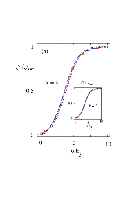
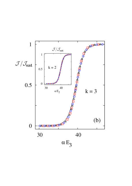
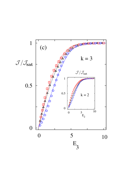
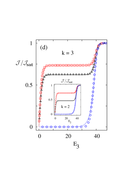
Figure 1: (Color online) Normalized SS currents for reconstructing trimers and dimers (insets) using ${\cal L}/L=1/2$. In listed order, the sectors of Table 2 here correspond to squares, triangles, and circles respectively. In (a) $T/J=1$, and (b) $T/J=0.1$, all data collapse onto the null string current (for clarity not shown), upon rescaling the drifts $E_{k}$ with $\alpha$’s such that $|1-\alpha|\lesssim 0.05$. The data are fitted by the mean field currents of Refs. Garrido ; Marro (solid lines), using the associated DLG densities referred to in Eq. (8). The mean field description extends as well to (c) $T/J=-1$, and (d) $T/J=-0.1$, where however all currents are sector dependent and DLG densities are chosen only as fitting parameters.

In Fig. 1 we show the resulting SS currents normalized to the saturation values of Table 2, after taking $T/J=\pm 1,\,\pm 0.1$, and ${\cal L}/L=1/2$ for several driving fields. In addition, Fig. 2 displays other plane of the current, in this case holding $E_{k}=10$ for a variety of temperatures, using both attractive and repulsive couplings.    It turns out that normalized currents of nonequivalent sublattices are indistinguishable within our error margins, a non obvious feature (except for random strings, as their sublattice occupations approach each other as ${\cal L}\to\infty$).

(i) $J>0$.– More importantly, under attractive interactions the currents of all studied sectors, both periodic and random, can be made to collapse into that of the null string by rescaling slightly the driving fields. This is displayed in Figs. 1a and 1b (random sectors not shown, for legibility). Furthermore, the data collapse extends also to the ${\cal J}-T$ plane provided the attractive couplings are taken slimly rescaled, as illustrated in Fig. 2a. It is noteworthy that in both ${\cal J}-E_{k}$ and ${\cal J}-T$ planes the null sector data follow very closely the mean field currents of the usual DLG Garrido . These arise essentially from a kinetic version of the cluster variation method applied to dynamics proceeding via exchange processes Marro . As expected from the arguments given in Sec. II A, here the fitting of the null string current is attained upon choosing $\rho_{\!{}_{\cal L}}=\left(1-\frac{\cal L}{L}\right)/\left[1+\frac{\cal L}{L}(k-1)\right]$ as the monomer density for the DLG system [see Eq. (8) ]. These numerical observations naturally lead us to put forward the universality hypothesis

$${\cal J}^{(i)}_{{}_{DRLG}}(E_{k},\,\beta J,\,{\cal L})/{\cal J}^{(i)}_{sat}=\frac{{\cal J}_{{}_{DLG}}(f\,E_{k},\,g\,\beta J,\,\rho_{\!{}_{\cal L}})}{\rho_{\!{}_{\cal L}}\left(1-\rho_{\!{}_{\cal L}}\right)}\;,\;J>0\,,$$ (22)

for normalized sublattice currents in ferromagnetic DRLG . Here, $f=f(\beta J)$ and $g=g(E_{k})$ are sector dependent scaling factors (probably close to 1), whereas ${\cal J}^{(i)}_{sat}$ is taken as in Eq. (10). Preliminary runs using other string lengths indicate similar results, thus adding more weight to this conjecture.

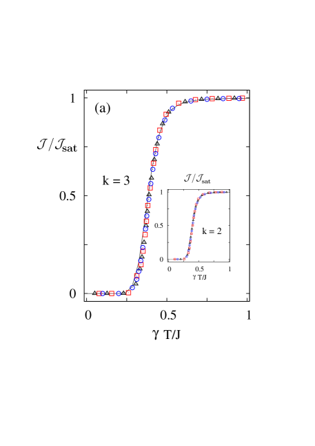
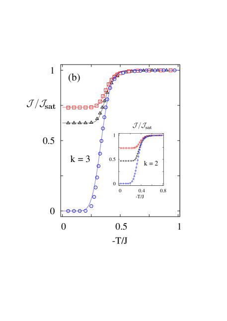
Figure 2: (Color online) Normalized SS currents versus temperature for $k=3$, and $k=2$ (insets) while keeping ${\cal E}k/T=10$ for (a) $J>0$, and (b) $J<0$. Key to symbols is the same as in Fig. 1. In (a) the data collapse is obtained by the rescale $J\to J/\gamma,$ choosing $\gamma$’s such that $|1-\gamma|\lesssim 0.02$. These currents follow closely the null string data (not displayed to avoid overcrowding). By contrast, in (b) all currents are sector dependent. In both cases the mean field fittings (Refs. Garrido ; Marro , solid lines) arise from the considerations given for Fig. 1.

(ii) $J<0$.– On the other hand, for repulsive interactions all normalized currents come out to be sector dependent, as is shown in Figs. 1c, 1d, and 2b, an aspect becoming more pronounced as temperature is lowered. However, this dependence appears to involve only the relative concentration of irreducible characters rather than their particular distributions, because in all situations the normalized currents of random sectors follow closely those of their periodic counterparts (alike the attractive case). Although these currents can also be fitted using the mean field approach to DLG Garrido ; Marro , the corresponding monomer densities can no longer be understood in terms of the ASEP analogy given before (except for null sectors and/or high drive regimes, as expected). Here, we merely use DLG densities as fitting parameters which actually turn out to be rather sensitive in tuning the values of the current plateaux exhibited in Figs. 1d, and 2b.

Further to universality issues, or the lack thereof for $J<0$, these results also suggest that DRLG currents inherit some of the salient features of DLG ones according to the type of interactions Garrido ; Marro (c.f. nevertheless pair correlations in non null sectors). For $J>0$ there is a continuous changeover from a rather insulating state at low temperatures and fields to a conducting phase as both $T$ and $\cal E$ are increased. For $J<0$ however, already at low temperatures some sectors can be found in conducting states, while exhibiting comparatively larger conductivities at small fields. As for the appearance of current plateaux in Figs. 1d, and 2b, notice that these are already present at the mean field level of the standard DLG.

III.2 Pair correlations

Turning to mesoscopic scales, in the following we focus on the SS instantaneous density-density correlation functions expressed through the subtracted or cummulant form

$$C(r)=\frac{1}{L}\,\sum_{j}\big{(}\,\langle\,n_{j}\,n_{j+r}\,\rangle-\rho_{\Lambda_{j}}\,\rho_{\Lambda_{j+r}}\big{)}\,,$$ (23)

with $\rho_{\Lambda_{i}}$ being the density of sublattice $\Lambda_{i}$. Also, to gain some further insight into the average organization of stationary regimes, we consider the static structure factor or Fourier transform of $C(r)$

$$S(q)=\frac{1}{L}\!\sum_{-L/2\,\leq\,r\,<\,L/2}\!\!\!\!\!\!\!\!\!e^{i\,q\,r}\,C(r)\,,$$ (24)

which in our case is a real function of the wavelength $\lambda=2\pi/q$. In Fig. 3 we first show this latter function for the case of dimers and trimers in the null sector, taking ${\cal L}/L=1/3$ and 1/4 in turn. At finite temperatures and far from the saturation or ASEP regime $|{\cal E}|\gg|J|$, the main maxima might be regarded as remnants of the periodicity and long range order of the Ising ground states. Clearly, in the attractive and repulsive situations these are respectively of the form $A_{k}^{L/(k+1)}A_{0}^{L/(k+1)}$ and $[A_{k}\,A_{0}]^{L/(k+1)}$ (along with translations), so as $T\to 0$ it is natural to expect sharp peaks at $q=0$ and $\frac{2\pi}{k+1}$ in each case. However, in general notice that when ${\cal L}/L\neq\frac{1}{k+1}$ the ground state of the null sector is highly degenerate for $J<0$ [ having the form $A_{k}^{m_{1}}A_{0}\,A_{k}^{m_{2}}A_{0}\cdots$ with $m_{j}\geq 0$  constrained as $\sum_{j}m_{j}=(L-{\cal L})/k$ ], thus setting a residual entropy which grows linearly with the system size. In fact, as temperature is lowered the structure factor remains essentially broad (see data of $T/J=-1/2$ for ${\cal L}/L=1/2$), and correlation lengths are of the order of the lattice spacing. A similar scenario arises in the monomer DLG, where degeneracies for $J<0$ and $\rho\neq 1/2$ also preclude long range order at any temperature Garrido ; Marro .

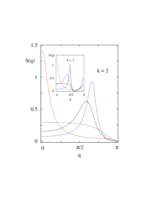
Figure 3: (Color online) Structure factors of sector $[A_{0}]^{\cal L}$ (null string) for dimers and trimers (inset), using ${\cal L}/L=$ 1/3 and 1/4 respectively. Solid, dashed, and dotted lines stand in turn for $(E_{k},T/J)=(2,\,-1),(2,\,1)$, and $(8,\,\pm 1)$. The two first cases exhibit maxima very near to $q=2\pi/3$ (dimers), $\pi/2$ (trimers), and 0 (both), thus resembling the average equilibrium periodicity of low temperature regimes. At high fields no periodicity takes over, regardless of the sign of $J$. The dashed-dotted lines denote the situation $(E_{k},T/J)=(2,\,-1/2)$ for ${\cal L}/L=$ 1/2, where the ground state is highly degenerate.

(i) $J<0$.– Yet, a rather different situation shows up for repulsive couplings in other periodic sectors also bearing high degeneracies. This is observed in Figs. 4a and 4b where, as an example, we illustrate respectively the behavior of strings $[A_{1}^{2}\,A_{0}]^{{\cal L}/5}$ ($k=2$), and $[A_{2}\,A_{1}A_{0}^{3}\,]^{{\cal L}/8}$ ($k=3$).

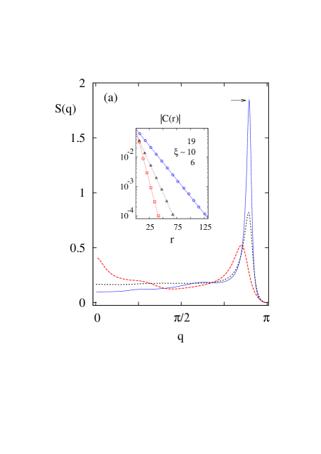
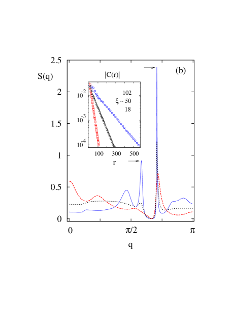
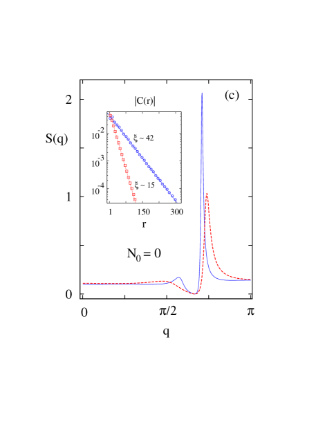
Figure 4: (Color online) Stationary structure factors for (a) dimers in sector $[A_{{}_{1}}^{2}A_{{}_{0}}]^{{\cal L}/5},$ (b) trimers in $[A_{{}_{2}}A_{{}_{1}}A_{{}_{0}}^{3}]^{{\cal L}/8},$ (c) trimers in energy conserving sectors $[A_{{}_{2}}^{2}A_{{}_{1}}]^{{\cal L}/8}$ (solid line, circles), and $[A_{{}_{2}}A_{{}_{1}}]^{{\cal L}/5}$ (dashed line, squares), using ${\cal L}/L=1/2$ throughout. Spatial correlation functions (insets) are highly oscillating, but only local maxima evidencing a decay $\propto e^{-r/\xi}$ are shown. Although (a) and (b) bear both highly degenerate ground states irrespective of the coupling sign, for $J<0$ the peaks marked by arrows rapidly grow as temperature is lowered. As in Fig. 3, here solid, dashed, and dotted lines (in turn, circles, squares, and triangles for insets) denote respectively the cases $(E_{k},T/J)=(2,\,-1),(2,\,1)$, and $(8,\,\pm 1)$. In the high field regime the results of (a) and (b) become independent of $T/J$, whereas in (c) this is always the case whether or not the system is driven.

It can be readily verified that for $J<0$ the number of ground states of the former grows exponentially with the lattice size so long as ${\cal L}/L\neq 5/7$, whereas that of the latter grows in the same manner provided ${\cal L}/L\neq 8/17$  (otherwise these states would be plain periodic sequences of the form $[\,A_{1}^{2}A_{2}\,A_{0}]^{L/7}$ for dimers, and $[\,A_{2}\,A_{1}\,(A_{3}\,A_{0})^{3}\,]^{L/17}$ for trimers). However, despite that exponential degeneracy the structure factors of both sectors can single out wavelengths exhibiting peaks that rapidly narrow and heighten as temperature is lowered. Also in lowering $T$, correlation lengths turn out to grow monotonically (e.g. at $T/J=-1/2$, $\xi\sim$ 500 in sector $[A_{2}\,A_{1}\,A_{0}^{3}\,]^{{\cal L}/8}$), while being already relatively large at $T/J=-1$ as compared with those of the case $J>0$ (see below). This is suggestive of an order-by-disorder scenario Villain in which thermal fluctuations are able to lift part of the degeneracy by selecting a subset of states with largest entropy in the ground state manifold. Here, note that the role of frustration in Refs. Villain is being played by the string conservation laws and the spatial extent of characters.

(ii) $J>0$.– By contrast, under attractive interactions no ordering seems to emerge for these sectors at low temperature regimes. Structure factors now remain basically flat (i.e. bounded) and correlation lengths do not increase as $T$ is lowered (Figs. 4a and 4b). Thus, thermal fluctuations now appear as being unable to suppress the residual entropy (also growing linearly in the thermodynamic limit of both sectors $\,\forall\,\,{\cal L}/L\neq 0^{+},1^{-})$ and no order-by-disorder seems likely to occur, just as in the situation of the null string and standard DLG under repulsive couplings. Similar results for $J>0$ were observed in the other sectors of Table 2, instead exhibiting effects of order by thermal fluctuations as long as the couplings are taken repulsive.

(iii) $|{\cal E}|\gg|J|$.– In approaching the ASEP or high field limit, pair correlations become progressively independent of the coupling values because all configurations tend to be equally likely. Already for $(E_{k},T/J)=(8,\pm 1)$, Figs. 3, 4a, and 4b indicate that all results are numerically indistinguishable. However as the field is lowered from the ASEP regime, for $J<0$ correlations can enhance significantly their ranges, in turn becoming arbitrarily long if temperatures are taken low enough. As displayed in Figs. 4a and 4b, this is to be contrasted with the opposite trend of both $\xi$ and $S(q)$ under attractive couplings, where the drive favors a slight increase of pair correlations.

(iv) $N_{0}=0$.– Finally, the ASEP regime is also related to the energy conserving sectors ($N_{0}=0$) referred to after Eq. (7), for which the presence of NN interactions is inconsequential. Despite the fact that every state is equally weighted, owing to the $k$-mer size here structure factors can still single out characteristic wave numbers (sector dependent) and exhibit large correlation lengths. This is illustrated in Fig. 4c. In the ASEP limit of the null sector these issues were recently analyzed in Ref. Gupta where closed expressions for general $k$’s were given for static correlations. Such rich behavior contrasts to that of totally uncorrelated monomers and dimers in sectors $[A_{1}]^{{\cal L}/2}$ (the only ones with $N_{0}=0$, which can be viewed as hopping monomers within one independent sublattice).

IV Concluding remarks

To summarize, we have discussed stationary aspects of driven lattice gases in which the role of biased monomers is played by extended and reconstructing $k$-mers under a Kawasaki dynamics [ Eq. (2) and Table 1 ]. Exploiting the correspondence between these processes and those involving the particle species defined in Eq. (3) we readily identified the many sector decomposition of the original problem, ultimately encompassed in the invariant ordering of these characters along the so called irreducible strings Menon ; BD . In the high field regime the dynamics of these new particles was thought of as an asymmetric exclusion process defined on a smaller lattice (Sec. II A), thereby enabling us to evaluate saturation currents [ Eq. (10) ] for generic strings or sectors of motion. In turn, the proliferation of these latter was shown to grow exponentially with the length of these strings (Sec. II B).

At finite temperatures and drives, we studied numerically the case of both dimers and trimers in typical sectors whose initial configurations were prepared by random sequential adsorption of ‘monomers’ in the equivalent ASEP states. These were then raised up into DRLG configurations, always keeping the distribution of irreducible characters or tagged ASEP ‘vacancies’ in each of the studied sectors (Table 2). The emerging stationary currents clearly discern between universal (Figs. 1a, 1b, 2a), and sector dependent behavior (Figs. 1c, 1d, 2b) according to the particle couplings being attractive or repulsive. In the former case, the universality hypothesis put forward in Eq. (22) suggests in turn an effective medium relation between generic sectors and null string currents via a slight rescale of drifts and interactions.

When it comes to mesoscopic levels of description (Sec. III B), also distinctive features appeared at low temperature regimes. In spite of the residual entropy in most of the studied sectors (stemming from their highly degenerate ground states), under repulsive couplings there is a substantial increase of both correlation lengths and structure factors at characteristic wavenumbers as temperature is lowered (Figs. 4a and 4b). We interpret these modes as being selected by thermal fluctuations from the ground state manifold thus giving rise, we suggest, to an order-by-disorder scenario Villain . For attractive interactions however, this latter can not be inferred from our simulations since, in line with the ground states degeneracies, both $\xi$ and $S(q)$ do not grow any further; a situation which resembles that of the standard DLG $(\rho\neq 1/2)$, and null strings $({\cal L}/L\neq\frac{1}{k+1})$ under repulsive couplings (Fig. 3). Finally, both large drive regimes and non-interacting sectors are governed by a simple product measure, but due to the $k$-mer size their correlation functions may show nontrivial oscillations and large correlation lengths (Figs. 4a, 4b, and 4c) Gupta .

It is natural to ask whether the above numerical findings could be approached theoretically. At the microscopic level of the master equation Kampen , the formal analogies between this latter and the Schrödinger equation describing the evolution of associated quantum spin chains have proven useful in the analysis of several nonequilibrium processes Schutz ; me . In fact, for vanishing drives and interactions these reconstructing systems have been studied in terms of spin-$\frac{1}{2}$ Heisenberg ferromagnets Menon , but for ${\cal E},\,\beta J\neq 0$ the evolution operators are neither familiar nor simple to analyze. On the other hand, already at the mean field level it is not clear how to proceed with an exponential number of conservation laws such as the IS’s discussed throughout.

Other issues not covered here that would be worth pursuing concern the phase ordering dynamics of periodic sectors under repulsive couplings where, as we have pointed out, stationary correlation lengths can get very large at low temperature regimes. It would be intersting to determine whether the dynamic exponents characterizing the large time growth of $\xi$ actually depend on the subspaces where the evolution takes place. There is also the question about tagged particle diffusion either with or without driving fields. For $\beta J=0$ and ${\cal E}\neq 0$ it is known that in the non-reconstructing case the root-mean-square displacement of a tagged particle around its mean position grows asymptotically in time as $\sim t^{1/2}$ (as usual), but if the bias is zero it grows anomalously slow as $\sim t^{1/4}\,$ Majumdar . In the reconstructing situation, where such caging effect might depend on the particular distribution of fragments of the sector considered, these issues remain quite open. The question also extends to the coarsening regime $-\beta J\gg 1$ for which other displacement laws might emerge depending on whether or not the motion is driven Godreche .

References

- (1) S. Katz, J. L. Lebowitz, and H. Spohn, Phys. Rev. B 28, 1655 (1983); J. Stat. Phys. 34, 497 (1984).
- (2) J. Marro, P. L. Garrido, and J. L. Vallés, Phase Transitions 29, 129 (1991); W. Dieterich, P. Fulde, and I. Peschel, Adv. Phys. 29, 527 (1980).
- (3) R. K. P. Zia, J. Stat. Phys. 138, 20 (2010); B. Schmittmann and R. K. P. Zia; Phys. Rep. 301, 45 (1998); also in Phase Transitions and Critical Phenomena, edited by C. Domb and J. L. Lebowitz (Academic Press, London, 1995), Vol. 17.
- (4) J. Marro and R. Dickman, Nonequilibirum Phase Transitions in Lattice Models, (Cambridge University Press, 1999), Chaps. 2 and 3.
- (5) B. Derrida, Phys. Rep. 301, 65 (1998); B. Derrida, M. Evans, V. Hakim, and V. Pasquier, J. Phys. A 26, 1493 (1993); R. A. Blythe and M. R. Evans, J. Phys. A 40, R333 (2007).
- (6) G. M. Schütz in Phase Transitions and Critical Phenomena, edited by C. Domb and J. L. Lebowitz (Academic Press, London, 2001), Vol. 19.
- (7) T. Chou and G. Lakatos, Phys. Rev. Lett. 93, 198101 (2004); L. B. Shaw, R. K. P. Zia, and K. H. Lee, Phys. Rev. E 68, 021910 (2003).
- (8) H. Schulz, G. Ódor, G. Ódor, and M. F. Nagyc, Comp. Phys. Comm. 182, 1467 (2011); S. L. A. de Queiroz and R. B. Stinchcombe, Phys. Rev. E 78, 031106 (2008); D. E. Wolf and L.-H. Tang, Phys. Rev. Lett. 65, 1591 (1990).
- (9) V. Popkov, L. Santen, A. Schadschneider, and G. M. Schütz, J. Phys. A 34, L45 (2001); D. Chowdhury, L. Santen, and A. Schadschneider, Phys. Rep. 329, 199 (2000).
- (10) K. Kawasaki, Phys. Rev. 145, 224 (1966); also in Phase Transitions and Critical Phenomena, edited by C. Domb and M.S. Green (Academic Press, New York, 1972), Vol. 2.
- (11) C. MacDonald, J. Gibbs, and A. Pipkin, Biopolymers 6, 1 (1968); C. MacDonald and J. Gibbs, Biopolymers 7, 707 (1969).
- (12) F. C. Alcaraz and R. Z. Bariev, Phys. Rev. E 60, 79 (1999); F. C. Alcaraz and M. J. Lazo, Braz. J. Phys. 33, 533 (2003).
- (13) G. I. Menon, M. Barma, and D. Dhar, J. Stat. Phys. 86, 1237 (1997).
- (14) D. Dhar, Physica A 315, 5 (2002); D. Dhar and J. L. Lebowitz, Eur. Phys. Lett. 92, 20008 (2010).
- (15) M. Barma, M. D. Grynberg, and R. B. Stinchcombe, J. Phys. Condens. Matter 19, 065112 (2007).
- (16) G. Schönherr and G.M. Schütz, J. Phys. A 37, 8125 (2004).
- (17) R. K. P. Zia, J. J. Dong and B. Schmittmann, J. Stat. Phys. 144, 405 (2011); J. J. Dong, B. Schmittmann, and R. K. P. Zia, Phys. Rev. E 76, 051113 (2007).
- (18) S. Gupta, M. Barma, U. Basu, and P. K. Mohanty, Phys. Rev. E 84, 041102 (2011).
- (19) In that latter respect but in the context of adsorption-desorption processes, consult also M. Barma and D. Dhar, Phys. Rev. Lett. 73, 2135 (1994); D. Dhar and M. Barma, Pramana – J. Phys. 41, L193 (1993).
- (20) Here we follow the approach given by P. L. Garrido, J. Marro, and R. Dickman in Ann. Phys. (NY) 199, 366 (1990), consult Sec. V. See also Ref. Marro .
- (21) J. Villain, R. Bidaux, J.-P. Carton, and R. Conte, J. Phys. (Paris) 41, 1263 (1980); E. F. Shender, Sov. Phys. JETP 56, 178 (1982); C. L. Henley, Phys. Rev. Lett. 62, 2056 (1989).
- (22) Other choices of rate functions include the usual Metropolis transition , as well as considered by H. van Beijeren and L. S. Schulman in Phys. Rev. Lett. 53, 806 (1984). In all cases detailed balance holds for , thus recovering the Boltzmann distribution.
- (23) N. G. van Kampen, Stochastic Processes in Physics and Chemistry, 3rd ed. (North Holland, Amsterdam, 2007), Chap. 5.
- (24) S. K. Lando, Lectures on Generating Functions, Student Mathematical Library, Vol. 23 (American Mathematical Society, Providence, 2003), Chap. 2.
- (25) O. Cohen and D. Mukamel, J. Phys. A 44, 415004 (2011); M. Clincy, B. Derrida, and M. R. Evans, Phys. Rev. 67, 066115 (2003); M. R. Evans, Y. Kafri, H. M. Koduvely, and D. Mukamel, Phys. Rev. Lett. 80, 425 (1998).
- (26) M. D. Grynberg, Phys. Rev. E 82, 051121 (2010).
- (27) S. N. Majumdar and M. Barma, Phys. Rev. B 44, 5306 (1991).
- (28) C. Godrèche and J. M. Luck, J. Phys. A 36, 9973 (2003).