Exact and approximate epidemic models on networks: a new, improved closure relation

Abstract

Recently, research that focuses on the rigorous understanding of the relation between simulation and/or exact models on graphs and approximate counterparts has gained lots of momentum. This includes revisiting the performance of classic pairwise models with closures at the level of pairs and/or triples as well as effective-degree-type models and those based on the probability generating function formalism. In this paper, for a fully connected graph and the simple $SIS$ (susceptible-infected-susceptible) epidemic model, a novel closure is introduced. This is done via using the equations for the moments of the distribution describing the number of infecteds at all times combined with the empirical observations that this is well described/approximated by a binomial distribution with time dependent parameters. This assumption allows us to express higher order moments in terms of lower order ones and this leads to a new closure. The significant feature of the new closure is that the difference of the exact system, given by the Kolmogorov equations, from the solution of the newly defined approximate system is of order $1/N^{2}$. This is in contrast with the $\mathcal{O}(1/N)$ difference corresponding to the approximate system obtained via the classic triple closure.

Keywords: Markov Chain; epidemic; pairwise model; pairwise closure

1 Introduction: exact stochastic models on and
of graphs

In this Section we present two important examples that motivate our investigations and a possible extension where progress can be made following some of the methods introduced in this paper. Here, we use a dynamical system type approach, where the Kolmogorov equations are simply considered as a system of linear ODEs with a transition rate matrix with specific properties such as special tri-diagonal structure and/or well defined functional form for the transmission rates. For example, consider a Markov chain with finite state space $\{0,1,\ldots,N\}$ and denote by $p_{k}(t)$ the probability that the system is in state $k$ at time $t$ (with a given initial state that is not specified at the moment). Assuming that starting from state $k$ the system can move to either state $k-1$ or to state $k+1$, the Kolmogorov equations of the Markov chain take the form

$$\dot{p}_{k}=a_{k-1}p_{k-1}-(a_{k}+c_{k})p_{k}+c_{k+1}p_{k+1},\quad k=0,\ldots,N.$$ (KE)

The first motivation for our study comes from epidemiology where a paradigm disease transmission model is the simple susceptible-infected -susceptible ($SIS$) model on a completely connected graph with $N$ nodes, i.e. all individuals are connected to each other. From the disease dynamic viewpoint, each individual is either susceptible ($S$) or infected ($I$) – the susceptible ones can be infected at rate $\tau$ if connected to an infected node, and the infected ones can recover at rate $\gamma$ and become susceptible again. It is known that in this case the $2^{N}$-dimensional system of Kolmogorov equations can be lumped to a $N+1$-dimensional system, see [12].

The lumped Kolmogorov equations take again the form (KE) with

$$a_{k}=\tau k(N-k),\quad c_{k}=\gamma k\quad\text{for}\quad k=0,\ldots,N\quad\text{with}\quad a_{-1}=c_{N+1}=0.$$ (1)

For homogeneous random graphs, where every node has $n(<N)$ links to other nodes in the network, a similar system can be written down. In this case the transition rates are as follows,

$$a_{k}=\tau nk\frac{N-k}{N-1},\quad c_{k}=\gamma k\quad\text{for}\quad k=0,\ldots,N\quad\text{with}\quad a_{-1}=c_{N+1}=0.$$ (2)

This equation is not exact in the sense that it is only an approximation to the exact process unfolding on a homogeneous random graph. This is not of immediate relevance as in this paper we concentrate on approximations of the Kolmogorov equations via low-dimensional ODEs, in particular we aim to derive approximate equations for the moments of the stochastic process described by the Kolmogorov equations.

A final example stems from a recent model of a dynamic network where links can be activated and deleted at random while subjected to a global constraint on the total number of links in the network (see Kiss et al. [7]). This example is a prerequisite to models where dynamics on the network is coupled with the dynamic of the network Gross and Blasius [3]. In the case of epidemic propagation on networks it is straightforward to assume that the propagation of the epidemic has an effect on the structure of the network. For example, susceptible individuals try to cut their links in order to minimise their exposure to infection. This leads to a change in network structure which in turn impacts on how the epidemic spreads. The first step in modelling this phenomenon is an appropriate dynamic network model such as the recently proposed globally-constrained Random Link Activation-Deletion (RLAD) model. This can be described in terms of Kolmogorov equations as follows,

$$\dot{p}_{k}(t) = \alpha(N-(k-1))\left(1-\frac{k-1}{K_{1}^{max}}\right)p_{k-1}(t)$$

$$- \left[\alpha(N-k)\left(1-\frac{k}{K_{1}^{max}}\right)+\omega k\right]p_{k}(t)+\omega(k+1)p_{k+1}(t),$$

$$k = 0,\ldots,N,$$

where $p_{k}(t)$ denotes the probability that at time $t$ there are $k$ active links in the network with $N$ denoting the total number of potential edges. It is assumed that non-active links are activated independently at random at rate $\alpha$ and that existing links are broken independently at random at rate $\omega$. Furthermore, the link creation is globally constrained by introducing a carrying capacity $K_{1}^{max}$, that is the network can only support a certain number of edges as given by $K_{1}^{max}$.

Using the above notation, here

$$a_{k}=\alpha(N-k)\left(1-\frac{k}{K_{1}^{\max}}\right),\quad c_{k}=\omega k,\quad\text{for}\quad k=0,\ldots,N\quad\text{with}\quad a_{-1}=c_{N+1}=0.$$ (3)

The common ingredient of all the models above is the set of Kolmogorov equations. Solving these even numerically, more often than not, is challenging and impossible simply due to the large number of equations. This has led to various approaches that set out to derive approximate models that are low-dimensional and can capture the exact dynamics in terms of the expected values of some well-defined quantities. These approaches could be broadly classified into heuristic and rigorous or semi-rigorous. For example, the original derivation of pairwise models was based on heuristic arguments [6]. More rigorous approaches include the lumping technique that exploits system symmetries and allows a significant reduction of the state space [12]. Additional models such as the effective degree models [1, 9] and the probability generating function approach by Volz [10, 14] led to excellent agreement with simulations without the explicit proof of convergence but with strong probabilistic arguments based on results by Kurtz [8].

In this paper, starting from the Kolmogorov equations, given by the simple $SIS$ epidemic model on a fully connected graph, the evolution equations for the moments are derived and are interpreted in terms of and compared to the classic pairwise equations. The equations for the moments are not self-contained, and a new/novel closure is proposed. This is based on the fact that the number of infecteds at all times is well approximated by a binomial distribution with time dependent parameters. The performance of the new closure is investigated numerically in the closing Section and we show that this is superior to the classic closure at the level of triples used for pairwise models.

2 Pairwise models: closure relations and their performance

It is of great interest to understand how and when the full set of Kolmogorov equations can be approximated via low-dimensional ODEs and also to assess the performance of the approximate models by, for example, working out the rate of convergence of the exact/full model towards the solution of the approximate or mean-field model or simply estimating the absolute difference between the two. Pairwise models have been widely used as an alternative or as a companion to simulations of epidemic models on mainly homogeneous random graphs. While originally, the pairwise equations have been heuristically defined, more recently, Simon et al. [12] and Taylor et al. [13] have shown that these can be derived directly from the exact Kolmogorov equations and that these pairwise equations are exact before closure on arbitrary graphs. Focusing on the simple $SIS$ type model, the first moment of the distribution is given by

$$[\dot{I}]=\tau[SI]-\gamma[I],$$ (4)

where $[I](t)=\sum_{k=0}^{N}kp_{k}(t)$. This is not a closed equation since $[SI]$ itself is a variable and an equation for this is needed. However, we can look for an approximation whereby the expected number of edges $[SI]\simeq e_{[SI]}([I])=[I](N-[I])$, that is, the expected number of ($SI$) pairs is estimated in terms of the number of the expected number of infecteds $[I]$. This now leads to a self-contained equation in terms of a new approximate variable $\tilde{I}$ given by

$$\dot{\tilde{I}}=\tau\tilde{I}(N-\tilde{I})-\gamma\tilde{I}.$$ (5)

This is the well known compartmental model for the $SIS$ epidemic.

The same argument can repeated by using a closure at the level of triples rather then pairs. In this case, the exact pairwise equations are given by

$$\frac{d[I]}{dt} = \tau[SI]-\gamma[I],$$ (6)

$$\frac{d[SI]}{dt} = \gamma([II]-[SI])+\tau([SSI]-[ISI]-[SI]),$$ (7)

$$\frac{d[II]}{dt} = -2\gamma[II]+2\tau([ISI]+[SI]),$$ (8)

$$\frac{d[SS]}{dt} = 2\gamma[SI]-2\tau[SSI].$$ (9)

Using the well know closure given by $[ABC]=\frac{N-2}{N-1}\frac{[AB][BC]}{[B]}$ (see [4, 6]) leads to the following approximate system

$$\dot{\overline{I}} = \tau\overline{SI}-\gamma\overline{I},$$ (10)

$$\dot{\overline{SI}} = \gamma(\overline{II}-\overline{SI})+\tau(\overline{SSI}-\overline{ISI}-\overline{SI}),$$ (11)

$$\dot{\overline{II}} = -2\gamma\overline{II}+2\tau(\overline{ISI}+\overline{SI}),$$ (12)

$$\dot{\overline{SS}} = 2\gamma\overline{SI}-2\tau\overline{SSI}.$$ (13)

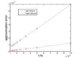
Figure 1: (a) Time evolution of the fraction infected (prevalence) based on the exact model and two different closures; pair and triple level. Here, $N=200$, $\gamma=2$ and $\beta=5$. (b) Approximation error (absolute value of the difference between the exact and two approximate models at steady state) plotted for different system sizes for the same transmission and recovery parameter values as at (a).

The focus now shifts from the derivation of the approximate model to whether and how well these agree with output from the exact system. More precisely, we will simply consider the difference between the exact solution $[I]$ and the approximate solutions $\tilde{I}$ and $\bar{I}$ in terms of the magnitude of $|[I](t)-\tilde{I}(t)|$ and $|[I](t)-\bar{I}(t)|$, and how these depend on population or network size. Numerical investigation reveals that the difference is of order $1/N$ for closures both at the level of pairs and triple. This is shown in Fig. 1, where both the exact (Eq. (KE) with coefficients given by Eq. (1)) and the approximate systems (i.e. with pairwise closure given by Eq. (5) and triple closure given by Eqs. (10)–(13)) have been solved numerically. This is somewhat surprising given that, at least intuitively, it is expected that the closure at the level of triples will be superior to that at the level of pairs. This numerical result can be made more rigorous at least for the closure at the level of pairs as shown by [2, 11].

3 Interpreting pairwise equations and closures in terms of moments

3.1 Equations for the moments

In this Section the analysis will focus on the derivation of the equations for the moments and the interpretation of the pairwise equations in terms of the moments. Let us define the $j$th moment associated with the stochastic process as follows

$$y_{j}(t)=\sum_{k=0}^{N}\left(\frac{k}{N}\right)^{j}p_{k}(t)\quad\text{or}\quad Y_{j}(t)=\sum_{k=0}^{N}k^{j}p_{k}(t),$$ (14)

where $N^{j}y_{j}=Y_{j}$ with $j=1,2,\ldots$. It is straightforward to derive evolution equations for the moments. For example, the derivative of the first moment, and in a similar way all others, can be given in function of other moments upon using the Kolmogorov equations (KE). The derivation for the first moment is outlined below,

$$\dot{Y}_{1}(t) = \sum_{k=0}^{N}k\dot{p}_{k}=\sum_{k=0}^{N}k(a_{k-1}p_{k-1}-(a_{k}+c_{k})p_{k}+c_{k+1}p_{k+1})$$

$$= \sum_{k=0}^{N}(ka_{k-1}p_{k-1}-ka_{k}p_{k}+kc_{k}p_{k}+kc_{k+1}p_{k+1}).$$

By changing the indices of the summation, plugging in the corresponding expressions for the transition rates $a_{k}$ and $c_{k}$ (Eq. (1)) and taking into account that $a_{-1}=c_{N+1}=0$ the following expression holds,

$$\dot{Y}_{1}(t)=\sum_{i=0}^{N}(\tau(i+i^{2})(N-i)-\tau i^{2}(n-i)-i^{2}\gamma+(i^{2}-i)\gamma)p_{i}.$$ (15)

Based on our notations (see, Eq. (14)), the equation above reduces to

$$\dot{Y}_{1}(t)=\tau NY_{1}-\tau Y_{2}-\gamma Y_{1}=(\beta-\gamma)Y_{1}-\frac{\beta}{N}Y_{2},$$ (16)

where $\beta=\tau N$ is the linking relation between mean-field-type and network models. Using a similar procedure, the equation for the second moment $Y_{2}$ can be easily computed and is given by

$$\dot{Y_{2}}=2(\beta-\gamma)Y_{2}-2\frac{\beta}{N}Y_{3}+(\beta+\gamma)Y_{1}-\frac{\beta}{N}Y_{2}.$$ (17)

Equations (16) & (17) can be recast in terms of the density dependent moments $y_{j}$s to give

$$\dot{y}_{1} = (\beta-\gamma)y_{1}-y_{2},$$ (18)

$$\dot{y}_{2} = 2(\beta-\gamma)y_{2}-2\frac{\beta}{N}y_{3}+\frac{1}{N}\left((\beta+\gamma)y_{1}-\beta y_{2}\right).$$ (19)

These equations will play a role that is similar to that of the pairwise equations, and similarly, these are also exact before a closure is applied, at some arbitrarily chosen moment. The above equations are not closed or self-contained since the second moment depends on the third and an equation for this is also needed. It is easy to see that this dependence of the moments on higher moments leads to an infinite but countable number of equations, see [2]. Hence, a closure is needed and in the next Section we will identify how the classic closure translates to a closure in moments, namely expressing $Y_{3}$ as a function of $Y_{1}$ and $Y_{2}$.

3.2 The equivalence between pairwise and moment equations

To be able to link the pairwise approach to the moment approach it is necessary to count the expected value of the singles, pairs and triples in terms of the moments. For a fully connected graph this is straightforward. For example, based on Eq. (14), the expected number of infecteds is given by

$$[I](t)=\sum_{k=0}^{N}kp_{k}(t)=Ny_{1}(t).$$ (20)

Similarly, it is easy to show that similar identities for pairs and triples can be derived. For example,

$$[SI](t)=\sum_{k=0}^{N}k(N-k)p_{k}(t)=N^{2}\sum_{k=0}^{N}\frac{k}{N}(1-\frac{k}{N})p_{k}(t)=N^{2}(y_{1}(t)-y_{2}(t)),$$ (21)

where, $k(N-k)$ simply denotes the number of ($SI$) pairs on a fully connected graph with $N$ nodes and $k$ infected individuals. For triples, the calculations are equally intuitive. For example, the expected number of $[SSI]$ triples can be counted by averaging over $(N-k)(N-k-1)k$ - the number of $[SSI]$ triples in the presence of $k$ infected nodes. Hence, the following relation holds,

$$[SSI](t) = \sum_{k=0}^{N}(N-k)(N-k-1)kp_{k}(t)$$ (22)

$$= N^{3}\sum_{k=0}^{N}\left(1-\frac{k}{N}\right)\left(1-\frac{k}{N}-\frac{1}{N}\right)\frac{k}{N}p_{k}(t)$$

$$= N^{3}\left(\left(1-\frac{1}{N}\right)y_{1}(t)+\left(\frac{1}{N}-2\right)y_{2}(t)+y_{3}(t)\right).$$

Following the same simple procedure as above, the following relations hold,

$$[S](t) = N(1-y_{1}(t)),$$ (23)

$$[II](t) = N^{2}\left(y_{2}(t)-\frac{1}{N}y_{1}(t)\right),$$ (24)

$$[SS](t) = N^{2}\left(1-\frac{1}{N}+\left(\frac{1}{N}-2\right)y_{1}(t)+y_{2}(t)\right),$$ (25)

$$[ISI](t) = N^{3}\left(-\frac{1}{N}y_{1}(t)+\left(\frac{1}{N}+1\right)y_{2}(t)-y_{3}(t)\right).$$ (26)

The results above allows us to test if the equations for the moments are consistent with the pairwise ones. Starting from the the equation for the expected number of infecteds and upon using Eq. (18), we obtain,

$$[\dot{I}](t)=N\dot{y}_{1}(t)=N((\beta-\gamma)y_{1}-y_{2})=N(\beta(y_{1}-y_{2})-\gamma y_{1})=\frac{\beta}{N}[SI]-\gamma[I].$$ (27)

The calculations above can be repeated for all other equations and these confirm the one-to-one correspondence between the moment and pairwise equations.

3.3 Interpreting closures via moments

The closure at the level of pairs and triples have to equally translate in a relation between the moments. First, the closure at the level of pairs is discussed. We look to use the pairwise closure $[SI]=[S][I]=(N-[I])[I]$ to obtain a relation between the moments. The simple relation above in terms of the moments translates to

$$N^{2}(y_{1}(t)-y_{2}(t))=N^{2}(y_{1}(t)-y_{1}^{2}(t))\Leftrightarrow y_{2}(t)=y_{1}^{2}(t).$$ (28)

For the triple closure the situation is different in that two different triples are closed, albeit using the same formal relation, and this could potentially lead to two different relations between the moments. The first triple closure, for the $SSI$ triple, upon using Eqs. (21)–(23) & (25), leads to the following relation,

$$\left(1-\frac{1}{N}\right)y_{1}+\left(\frac{1}{N}-2\right)y_{2}+y_{3}=\frac{N-2}{N-1}\frac{\left(1-\frac{1}{N}+\left(\frac{1}{N}-2\right)y_{1}+y_{2}\right)(y_{1}-y_{2})}{1-y_{1}}.$$ (29)

The equation above, after some algebra, yields a closure at the level of the moments and $y_{3}$ can be given in function of the previous two moments as follows,

$$y_{3}=-\frac{1}{N}y_{1}+(1+\frac{1}{N})y_{2}-\frac{N-2}{N-1}\frac{(y_{1}-y_{2})^{2}}{1-y_{1}}.$$ (30)

It is worth noting that the closure for $[ISI]$ yields the same closure relation for the third moment.

4 The new, improved closure and its performance

The novel closure put forward here is based on the empirical observation that $p_{k}(t)$ is well approximated by a binomial distribution $\mathcal{B}(n,p)$, where $n$ and $p$ depend on time and will specified in terms of the moments of the distribution. The first three moments of the binomial distribution can be specified easily in terms of the two parameters and are as follows,

$$Y_{1} = np$$ (31)

$$Y_{2} = np+n(n-1)p^{2}$$ (32)

$$Y_{3} = np+3n(n-1)p^{2}+n(n-1)(n-2)p^{3}.$$ (33)

Using Eqs. (31) & (32), $n$ and $p$ can be expressed in term of $Y_{1}$ and $Y_{2}$ as follows,

$$p=1+Y_{1}-\frac{Y_{2}}{Y_{1}},\qquad n=\frac{Y_{1}^{2}}{Y_{1}+Y_{1}^{2}-Y_{2}}.$$ (34)

Plugging the expressions for $p$ and $n$ (Eq. 34) into Eq. (33), the closure for the third moment is found to be

$$Y_{3}=\frac{2Y_{2}^{2}}{Y_{1}}-Y_{2}-Y_{1}(Y_{2}-Y_{1}).$$ (35)

This relation defines the new triple closure and in terms of the density dependent moments is equivalent to

$$y_{3}=\frac{2y_{2}^{2}}{y_{1}}-y_{1}y_{2}+\frac{1}{N}(y_{1}^{2}-y_{2}).$$ (36)

Using the equations for the first moment (18) the closure at the level of the pairs yields the following approximate equation

$$\dot{x}_{1}=(\beta-\gamma)x_{1}-\beta x_{1}^{2}.$$ (37)

Using the equations for the first two moments ((18) & (19)) and the closure at the level of the third moment yields

$$\dot{x_{1}} = (\beta-\gamma)x_{1}-\beta x_{2},$$ (38)

$$\dot{x_{2}} = 2(\beta-\gamma)x_{2}-2\beta x_{3}+\frac{1}{N}((\beta+\gamma)x_{1}-\beta x_{2}),$$ (39)

where

$$x_{3}=\frac{2x_{2}^{2}}{x_{1}}-x_{1}x_{2}+\frac{1}{N}(x_{1}^{2}-x_{2}).$$ (40)

Moreover, we can also define a simplified binomial closure by neglecting the order $1/N^{2}$ in the full binomial closure, provided also that $x_{1}^{2}-x_{2}$ is of $\mathcal{O}(1/N)$. This will lead to

$$x_{3}=3x_{1}x_{2}-2x_{1}^{3},$$ (41)

with all the above in contrast with the the classic triple closure given by Eq. (30).

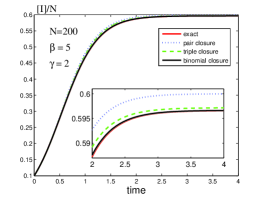
Figure 2: (a) Time evolution of the fraction infected (prevalence) based on the exact model and three different closures; pair, triple level and the binomial closure. Here, $N=200$, $\gamma=2$ and $\beta=5$. (b) Approximation error (absolute value of the difference between the exact and approximate models at steady state given by the triple and binomial closures) plotted for different system sizes for the same transmission and recovery parameter values as at (a). It is worth noting that the $x$-axis in (b) is in terms of $1/N^{2}$ as opposed to $1/N$ as in Fig. 1(b).

The current setup allows us to compare the exact model as given by the Kolmogorov equations (KE) with transition rates given by Eq. (1) to three different approximate models. The first results from the pairwise closure and is given by Eq. (5). The second is a direct consequence of the closure at the level of triples and is given by Eqs. (10)–(13). Finally, the third approximate system results from the novel binomial closure (see Eq. (36)) with the approximate system defined by Eqs. (38)–(40). The elegance of this approach stems from the fact that all numerical results are free from simulations and rely solely on the time integration of ODE systems. In Fig. 1, plots of the time evolution together with the approximation errors are given for the classic approximate models corresponding to pairwise and triple closure. The most significant feature of this plot is the order $1/N$ approximation error independently of the closure. The same approximation error suggests qualitative similarity between the two approximate models and it somewhat surprising that the closure at the level of triples produces no immediately obvious benefits or qualitatively different behaviour. In contrast, in Fig. 2 the performance of the binomial closure is compared to the triple closure. The approximation error plot in Fig. 2b is the most significant as it shows numerical evidence that the binomial closure performs significantly better with error that is of order $1/N^{2}$. While we were not yet able to prove analytically this result, for the case of pairwise closure we gave rigorous proof in [2, 11], where the result is more general as apart from estimating the approximate error at the steady state also extends to the approximate error at different times.

The quantitative comparison of the different closure relations is shown in Table 1. Her, the values of the steady states obtained for the different closures are compared to the exact value of the stationary prevalence. The advantage of comparing the steady state values is that these can be given analytically without solving ODEs numerically. The steady state from the pairwise closure Eq. (5) is

$$\frac{\tilde{I}_{ss}}{N}=1-\frac{\gamma}{\beta},$$ (42)

where $\beta=\tau N$. The steady state from the triple closure Eqs. (10)–(13) is

$$\frac{\overline{I}_{ss}}{N}=(N-1)\frac{(N-2)\beta-N\gamma}{(N-1)(N-2)\beta-N\gamma}.$$ (43)

The steady state from the binomial closure Eqs. (38)–(40) is

$$\frac{I^{*}_{ss}}{N}=\frac{Nq^{2}-1}{Nq-1},$$ (44)

where $q=1-\gamma/\beta$. Finally, the value of the steady state from the Kolmogorov equations (KE) can be derived as

$$\frac{[I]_{ss}}{N}=\frac{\sum\limits_{k=0}^{N-1}(k+1)A_{k}}{N\sum\limits_{k=0}^{N-1}A_{k}},$$ (45)

where $A_{0}=1$ and

$$A_{k}=\frac{\beta^{k}(N-1)(N-2)...(N-k)}{\gamma^{k}(k+1)N^{k}},\quad k=1,2,\ldots N-1.$$

The approximation errors shown in Table 1 are

$$\left|\frac{\tilde{I}_{ss}}{N}-\frac{[I]_{ss}}{N}\right|,\quad\left|\frac{\overline{I}_{ss}}{N}-\frac{[I]_{ss}}{N}\right|,\quad\left|\frac{I^{*}_{ss}}{N}-\frac{[I]_{ss}}{N}\right|.$$

In the Table these values are multiplied by 1000 to get numerical values closer to 1. Using the analytical expressions above it is easy to show that $\frac{\overline{I}_{ss}}{N}\rightarrow\frac{\tilde{I}_{ss}}{N}$ and $\frac{I^{*}_{ss}}{N}\rightarrow\frac{\tilde{I}_{ss}}{N}$ when $N\rightarrow\infty$. However, we did not yet manage to formally prove that

$$\left|\frac{\tilde{I}_{ss}}{N}-\frac{[I]_{ss}}{N}\right|/N,\quad\left|\frac{\overline{I}_{ss}}{N}-\frac{[I]_{ss}}{N}\right|/N,\quad\left|\frac{I^{*}_{ss}}{N}-\frac{[I]_{ss}}{N}\right|/N^{2}$$

all tend to a non-zero number as $N$ gets large and thus analytically confirming the $\mathcal{O}(1/N)$ and $\mathcal{O}(1/N^{2})$ errors.

5 Discussion

In this paper, we proposed a novel/new closure that produces qualitatively different results when compared to the classic closure. Namely, the difference between the exact system from the solution of the approximate model that results from the binomial closure is smaller (i.e. $\mathcal{O}(1/N^{2})$ compared to $\mathcal{O}(1/N)$) and this has been illustrated via numerical examples. The paper has also identified the link between the equations of the moments and pairwise equations. In particular, it is worth noting that in terms of moments, the pairwise equations reduce to two simple ODEs and this is in contrast with four equations for the pairwise model. However, this apparent discrepancy is not as marked since the pairwise model can be easily reduced to three equations by noting that, for example, $[SS]=(N-1)(N-[I])-[SI]$. This still leaves one extra equation in the pairwise model when compared to the equivalent system in terms of moments. This suggests that the three equations are not completely independent in some sense that is not easy to define or pinpoint.

The present study also allows us to make a few more important observations. For example, one can attempt to close the moment equations at the second moment but, without using the equivalent closure that follows from the pairwise model. This can be achieved by considering the limiting case of $n=N$ and expressing the second moment in terms of the first. This will lead to a new closure at the level of pairs but, this performs similarly to the classic closure at the pair level.

The procedure that we illustrate in this paper can be generalised and applied within the general context of model reduction, where Kolmogorov-type systems are reduced to approximate models with far fewer equations. Our method is based on a semi-heuristic argument which relies on the assumption that the distribution of the stochastic process in time can be well-approximated by some theoretical distribution with time-dependent parameters. Moreover, the distribution has to be such that there is a unique, one-to-one correspondence between the moments and the parameters of the distribution. If the conditions above hold, the theoretical distribution will determine the exact type of closure that is necessary to obtain a reduction in the number of equations. The method also allow us to close at different levels or moments and to explore the benefits of closing at higher order moments. While the initial results and applicability of our method is promising (see example below for the homogeneous random graph case), we are yet to fully explore the applicability of our method or to identify the sufficient and/or necessary requirements that guarantees that the proposed closure or reduction procedure will be applicable. It is worth noting that here the main focus in not on the approximation of simulation results corresponding to a stochastic process but rather the model reduction where the Kolmogorov equations are already given.

Our result about the new closure relation applies directly to homogeneous random graphs provided that the Kolmogorov equations for this case take the form given in Eq. (KE) with coefficients defined in Eq. (2). The formulation of the result is even more straightforward if the following slight modification for the transmission rate $a_{k}$ is introduced

$$a_{k}=\tau nk\frac{N-k}{N}.$$

In this case, the coefficients $a_{k}$ and $c_{k}$ in Eq. (1) and Eq. (2) are formally equivalent, i.e. both can be written as $a_{k}=\frac{\delta}{N}k(N-k)$ with $\delta=\beta$ for the complete graph, and $\delta=\tau n$ for the homogeneous random graph. It is worth noting that, in the case of the complete graph, $\tau$ is of order $1/N$ and $\beta$ is independent of $N$, while for the homogeneous random graph, $\tau$ is independent of $N$. However, in both cases the coefficient $a_{k}$ can be given as the product of $k(N-k)$ with a $1/N$ term. Therefore in the case of a homogeneous random graph the equation for the moments can be easily obtained from Eqs. (18) & (19) by writing $\tau n$ instead of $\beta$. Thus the ODE system with the binomial closure for the homogeneous random graph is the same as Eqs. (38)–(40) following a change that again replaces $\beta$ with $\tau n$.

While there are some limitations to the straightforward extension of our results to arbitrary graphs and/or dynamics, the present paper provides the basis for some more rigorous analysis as well as the possibility of deriving new closures. As such, this study offers a new or different direction that can lead to further progress in the area of approximating stochastic processes independently of whether these involve graphs.

N	100	200	400	800
1000 $\times$ pair appr. err.	6.9486	3.4008	1.6832	0.8374
1000 $\times$ triple appr. err.	1.2355	0.5729	0.2763	0.1357
1000 $\times$ binomial appr. err.	0.1689	0.0395	0.0096	0.0024

Table 1: Numerical values for the discrepancy between the exact and approximate solutions for different network sizes.

References

- [1] F. Ball & P. Neal 2008. Network epidemic models with two levels of mixing. Math. Biosci. 212, 69-87.
- [2] A. Bátkai, I.Z. Kiss, E. Sikolya & P.L. Simon 2011. Differential equation approximations of stochastic network processes: an operator semigroup appraoch. Submitted to Networks and heterogeneous media.
- [3] T. Gross & B. Blasius 2008. Adaptive coevolutionary networks: a review, J. Roy. Soc. Interface 5, 259-271.
- [4] T. House & M. J. Keeling 2010. The impact of contact tracing in clustered populations, PLoS Computational Biology 6:3 e1000721.
- [5] T. House & M. J. Keeling 2011. Insights from unifying modern approximations to infections on networks, J. Roy. Soc. Interface 8, 67-73.
- [6] M.J. Keeling 1999. The effects of local spatial structure on epidemiological invasions, Proc. R. Soc. Lond. B 266, 859-867.
- [7] I.Z. Kiss, L. Berthouze, T.J. Taylor & P.L. Simon 2011. Modelling approaches for simple dynamic networks and applications to disease transmission models. Submitted to Proc. Roy. Soc A.
- [8] T.G. Kurtz 1970. Solutions of ordinary differential equations as limits of pure jump Markov processes. J. Appl. Prob. 7, 49-58.
- [9] J. Lindquist, J. Ma, P. van den Driessche & F.H. Willeboordse 2011. Effective degree network disease models, J. Math. Biol. 62, 143-164.
- [10] J. C. Miller 2011. A note on a paper by Erik Volz: SIR dynamics in random networks. J. Math. Biol. 62, 349-358.
- [11] P. L. Simon & I. Z. Kiss 2011. From exact stochastic to mean-field ODE models: a case study of three different approaches to prove convergence results. Submitted to IMA Journal of Applied Mathematics.
- [12] P.L. Simon, M. Taylor & I.Z. Kiss 2011. Exact epidemic models on graphs using graph-automorphism driven lumping. J. Math. Biol. 62, 479-508.
- [13] M. Taylor, P. L. Simon, D. M. Green, T. House & I. Z. Kiss 2011. From Markovian to pairwise epidemic models and the performance of moment closure approximations, Accepted for publication in J. Math. Biol. and available at http://www.maths.sussex.ac.uk/cgi-bin/World/preprints/contents.cgi?id=116.
- [14] E. Volz 2008. SIR dynamics in structured populations with heterogeneous connectivity. J. Math. Biol. 56, 293-310.