Impact of Step Defects on Surface States of Topological Insulators

Abstract

The eigenstates in the presence of a step defect (SD) along $x$ or $y$ axis on the surface of topological insulators are exactly solved. It is shown that unlike the electronic states in conventional metals, the topological surface states across the SD can produce spin rotations. The magnitudes of the spin rotations depend on the height and direction of the SD. The oscillations of local density of states (LDOS) are characterized by a wave vector connecting two points on the hexagonal constant-energy contour at higher energies. The period of the oscillation caused by the SD along $y$ axis is $\sqrt{3}$ ($\frac{1}{\sqrt{3}}$) times that induced by the SD along $x$ axis at a larger positive (negative) bias voltage. With increasing the bias voltage, the period of the oscillation, insensitive to the strength of the SD, becomes smaller. At lower energies near the Fermi surface, the two types of wave vectors coexist in the LDOS modulations. These results are consistent qualitatively with recent observations of scanning tunneling microscopy.

Recently topological surface states have attracted much attention in the condensed matter community due to their potential applications in quantum computing or spintronics [1,2]. The novel electronic states, which preserve time-reversal symmetry, are produced by spin-orbit interactions. Such Dirac-cone-like surface states have been observed in three dimensional bulk insulating materials, such as Bi_1-xSb_x [3], Bi₂Sb₃ [4], Sb₂Te₃ [5], Bi₂Te₃ [5,6], TlBiSe₂ and TlBiTe₂ [7], by angle-resolved photoemission spectroscopy (ARPES). The surface energy band structure was determined by employing $k\cdot p$ theory [8], where an unconventional hexagonal warping term plays a crucial role in explaining the ARPES observations.

Scanning tunneling microscopy (STM) experiments have probed the electronic waves in the presence of step defect (SD) on the surface of the topological insulators Bi₂Te₃ [9,10] and the antimony (Sb) [11,12]. The absence of backscattering of the topological surface states makes the local density of states (LDOS) near the SD more extraordinary as compared to that on the surface of conventional metals [13,14]. In Ref. [10], Alpichshev et al. observed the oscillations of the LDOS near a SD, dispersing with a wave vector that may result from a hexagonal warping term. With increasing the bias voltage, the period of the LDOS modulation decreases. In this work, we investigate electron transport in the presence of a SD along $x$ or $y$ axis on the surface of topological insulators in the framework of quantum mechanics in order to explain the STM experiments. We treat the SD as a $\delta(y)$ or $\delta(x)$ potential barrier, similar to that in conventional metals [13,14]. We note that in Ref. [15], the authors studied the scattering from a $\delta(x)$ in strong topological insulators. However, they didn’t take the hexagonal warping term into account, which is the key to understand the STM observations [9-12].

The momentum space Hamiltonian describing the surface states of topological insulators reads [8]

$$H=(\frac{k^{2}}{2m^{*}}-\mu)I+v(k_{x}\sigma_{y}-k_{y}\sigma_{x})+\lambda\phi(k_{x},k_{y})\sigma_{z},$$

where $I$ and $\sigma_{i}(i=x,y,z)$ are the $2\times 2$ unit matrix and the Pauli matrices, respectively, $m^{*}$ is the effective mass of electrons, which is usually very large for the topological insulators, $\mu$ is the chemical potential, $v$ is the strength of the Rashba spin-orbit coupling, the last term is the so called hexagonal warping term, and $\phi(k_{x},k_{y})=k_{x}(k_{x}^{2}-3k_{y}^{2})$. We note that the real space Hamiltonian corresponding to Eq. (1) can be obtained by taking the transformations: $k_{x}=-i\frac{\partial}{\partial x}$ and $k_{y}=-i\frac{\partial}{\partial y}$. Obviously, the Hamiltonian (1) has the eigenenergies

$$E_{{\bf k}s}=\frac{k^{2}}{2m^{*}}+(-1)^{s}{\cal E}_{\bf k}-\mu$$

with $s=0$ and $1$, and ${\cal E}_{\bf k}=\sqrt{\lambda^{2}\phi^{2}(k_{x},k_{y})+v^{2}k^{2}}$.

We can see easily that $x$ and $y$ directions in the Hamiltonian (1) are inequivalent due to the existence of the warping term. Therefore, it is naturally expected that different orientation of SD leads to different oscillatory features in the LDOS. In the following we study two special SDs, which are usually observed in STM experiments.

SD along $y$ axis. We first consider the SD along $y$ axis, which can be described by the $\delta$ potential $U(x)=U_{0}\delta(x)$ [13,14]. Here $U_{0}$ is the strength of the SD and is usually weak, but $m^{*}U_{0}$ has a finite value.

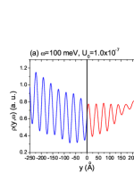
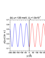
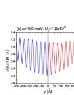
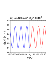
Figure 1: (Color online) The LDOS $\rho_{I,II}(x,\omega)$ as a function of distance from the line defect along $y$ axis with different values of $m^{*}U_{0}$ and bias voltages.

The wave function at the left of the SD, i.e. $x<0$, is

$$\psi_{I}^{s}(x,y;{\bf k})=\frac{e^{i(k_{x}x+k_{y}y)}}{\Gamma_{s}(k_{x},k_{y})}\left(\begin{array}[]{c}\xi_{s}(k_{x},k_{y})\\ v(ik_{x}-k_{y})\end{array}\right)$$

$$+R_{s}\cdot\frac{e^{i(-k_{x}x+k_{y}y)}}{\Gamma_{s}(-k_{x},k_{y})}\left(\begin{array}[]{c}\xi_{s}(-k_{x},k_{y})\\ v(-ik_{x}-k_{y})\end{array}\right),$$

where $\xi_{s}(k_{x},k_{y})=\lambda\phi(k_{x},k_{y})+(-1)^{s}{\cal E}_{\bf k},$ $\Gamma_{s}(k_{x},k_{y})=\sqrt{\xi_{s}^{2}(k_{x},k_{y})+v^{2}k^{2}}$, the first and second terms represent the incoming and reflection wave functions, respectively, while the outcoming wave function at the right of the SD, i.e. $x>0$, is found to have general form

$$\psi_{II}^{s}(x,y;{\bf k})=T_{s}\cdot\frac{e^{i(k_{x}x+k_{y}y)}}{\Gamma_{s}(k_{x},k_{y})}\left(\begin{array}[]{c}\xi_{s}(k_{x},k_{y})\\ v(ik_{x}-k_{y})\end{array}\right)$$

$$+e^{ik_{y}y}\left(\begin{array}[]{c}A_{s}\cos(k_{x}x)+B_{s}\sin(k_{x}x)\\ C_{s}\cos(k_{x}x)+D_{s}\sin(k_{x}x)\end{array}\right),$$

where $C_{s}$ and $D_{s}$ are arbitrary constants to be determined by the boundary conditions at the SD, i.e. $x=0$, and

$$A_{s}=-u_{s}C_{s}-v_{s}D_{s},~{}~{}~{}~{}~{}B_{s}=v_{s}C_{s}-u_{s}D_{s},$$

$$u_{s}=(vk^{2})^{-1}[i\lambda k_{x}\phi(k_{x},k_{y})+(-1)^{s}k_{y}{\cal E}_{\bf k}]$$

$$v_{s}=(vk^{2})^{-1}[-i\lambda k_{y}\phi(k_{x},k_{y})+(-1)^{s}k_{x}{\cal E}_{\bf k}].$$

We note that the first term in Eq. (4) is the tunneling wave function while the second term describes an extra spin rotation, distinguishing from the electronic wave function in conventional metals. It is nothing but this term that leads to the oscillations of the LDOS at $x>0$ [11].

Integrating the coupled Schrodinger equations associated with the Hamiltonian (1) in real space plus the $\delta(x)$ potential, we have the boundary conditions at the SD,

$$\psi_{I}^{s}(0,y;{\bf k})=\psi_{II}^{s}(0,y;{\bf k})$$

$$\frac{\partial\psi_{II}^{s}(0,y;{\bf k})}{\partial x}-\frac{\partial\psi_{I}^{s}(0,y;{\bf k})}{\partial x}=2m^{*}U_{0}\psi_{I}^{s}(0,y;{\bf k}).$$

Substituting Eqs. (3) and (4) into Eq. (6), we obtain the spin rotation constants

$$C_{s}=-\frac{m^{*}U_{0}\eta_{s}^{+}}{\Gamma_{s}(k_{x},k_{y})k_{x}(ik_{x}-m^{*}U_{0})}\cdot\frac{k_{x}[\xi_{s}(k_{x},k_{y})+u_{s}v(ik_{x}-k_{y})]+v_{s}(ik_{x}-2m^{*}U_{0})v(ik_{x}-k_{y})}{v^{2}k^{2}(1+u_{s}^{2}+v_{s}^{2})+u_{s}\eta_{s}^{-}+iv_{s}\eta_{s}^{+}},$$

$$D_{s}=-\frac{m^{*}U_{0}\eta_{s}^{+}}{\Gamma_{s}(k_{x},k_{y})k_{x}(ik_{x}-m^{*}U_{0})}\cdot\frac{v_{s}k_{x}v(ik_{x}-k_{y})-(ik_{x}-2m^{*}U_{0})[\xi_{s}(k_{x},k_{y})+u_{s}v(ik_{x}-k_{y})]}{v^{2}k^{2}(1+u_{s}^{2}+v_{s}^{2})+u_{s}\eta_{s}^{-}+iv_{s}\eta_{s}^{+}},$$

where $\eta_{s}^{\pm}=\xi_{s}(-k_{x},k_{y})v(ik_{x}-k_{y})\pm\xi_{s}(k_{x},k_{y})v(ik_{x}+k_{y})$, and the reflection and tunneling coefficients

$$R_{s}=\frac{\Gamma_{s}(-k_{x},k_{y})}{\eta_{s}^{+}}[A_{s}v(ik_{x}-k_{y})-C_{s}\xi_{s}(k_{x},k_{y})],$$

$$T_{s}=1-\frac{\Gamma_{s}(k_{x},k_{y})}{\eta_{s}^{+}}[A_{s}v(ik_{x}+k_{y})+C_{s}\xi_{s}(-k_{x},k_{y})].$$

Obviously, when $U_{0}=0$, we have $C_{s}=D_{s}=R_{s}=0$ and $T_{s}=1$.

In order to compare with the STM experiments, we calculate the LDOS near the SD, which can be expressed as

$$\rho_{I,II}(x,\omega)=\sum_{k_{x}>0,k_{y},s}|\psi_{I,II}^{s}(x,y;{\bf k})|^{2}\delta(\omega-E_{{\bf k}s}).$$

Here we emphasize that the formula (9) only considers the contributions of the topological surface states with $k_{x}>0$ so that we can know clearly the LDOS modulations induced by the incoming and reflection wave functions or the outcoming wave function. We note that the LDOS observed by STM experiments should also include the contributions coming from those surface states with $k_{x}<0$, i.e. $\rho_{\rm STM}(|x|,\omega)=\rho_{I}(x,\omega)+\rho_{II}(x,\omega)$. In our following calculations, we use the physical parameters of the topological insulator Bi₂Te₃: $\lambda=250.0$ eV$\cdot$ų, $v=2.55$ eV$\cdot$ų, and $\mu=0.334$ eV [8,10]. In Fig. 1, we present the LDOS with different values of $m^{*}U_{0}$ at high positive and negative energies. Obviously, the amplitude of the LDOS modulation near the SD depends strongly on the strength $U_{0}$ of the $\delta$ potential and the bias voltage $\omega$. However, if $\omega$ is fixed, both period and phase of the oscillation keep unchanged with increasing $U_{0}$. When $\omega=100$ meV, the period $T_{y}(\omega)\approx 58.0$ Åin both sides of the SD. When $\omega=-120$ meV, the period $T_{y}(\omega)\approx 42.0$ Å. At the positions with the same distance from the SD, the LDOS at these bias voltages has a maximum value and a minimum value, respectively.

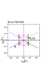
In order to understand the oscillatory features of the LDOS, we plot the constant-energy contours of the topological surface state band at $\omega=100$ meV and $-120$ meV in Fig. 2. We observe that the periods of the LDOS modulations at these energies are associated with a wave vector connecting two points on the corresponding constant-energy contours. In other words, $T_{y}(100)\sim\frac{2\pi}{|{\bf q}_{A}-{\bf q}_{B}|}=\frac{2\pi}{|{\bf q}_{C}-{\bf q}_{D}|}=\frac{\pi}{0.0549}=57.2$ Å, and $T_{y}(-120)\sim\frac{2\pi}{|{\bf q}_{E}-{\bf q}_{F}|}=\frac{2\pi}{|{\bf q}_{G}-{\bf q}_{H}|}=\frac{\pi}{0.0727}=43.2$ Å. Therefore, such oscillations of the LDOS are due to quasiparticle interference. It is obvious that there is no backscattering of the topological surface states in the LDOS, which is associated with the wave vector connecting two crossing points between the constant-energy contour and the $x$ axis.

Figure 2: (Color online) The constant-energy contours of the surface state band at different energies.

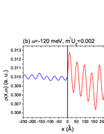
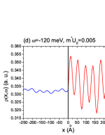
SD along $x$ axis. Now we consider the SD along $x$ axis, corresponding to that observed in Bi₂Te₃ by the STM experiment [10]. Similarly, the wave function at $y<0$ has the form

$$\psi_{I}^{s}(x,y;{\bf k})=\frac{e^{i(k_{x}x+k_{y}y)}}{\Gamma_{s}(k_{x},k_{y})}\left(\begin{array}[]{c}\xi_{s}(k_{x},k_{y})\\ v(ik_{x}-k_{y})\end{array}\right)$$

$$+{\cal R}_{s}\cdot\frac{e^{i(k_{x}x-k_{y}y)}}{\Gamma_{s}(k_{x},k_{y})}\left(\begin{array}[]{c}\xi_{s}(k_{x},k_{y})\\ v(ik_{x}+k_{y})\end{array}\right),$$

where we have used $\xi_{s}(k_{x},-k_{y})\equiv\xi_{s}(k_{x},k_{y})$ and $\Gamma_{s}(k_{x},-k_{y})\equiv\Gamma_{s}(k_{x},k_{y})$. The wave function at $y>0$ is

$$\psi_{II}^{s}(x,y;{\bf k})={\cal T}_{s}\cdot\frac{e^{i(k_{x}x+k_{y}y)}}{\Gamma_{s}(k_{x},k_{y})}\left(\begin{array}[]{c}\xi_{s}(k_{x},k_{y})\\ v(ik_{x}-k_{y})\end{array}\right)$$

$$+e^{ik_{x}x}\left(\begin{array}[]{c}{\cal A}_{s}\cos(k_{y}y)+{\cal B}_{s}\sin(k_{y}y)\\ {\cal C}_{s}\cos(k_{y}y)+{\cal D}_{s}\sin(k_{y}y)\end{array}\right),$$

where ${\cal A}_{s}=w_{s}(k_{x}{\cal C}_{s}-k_{y}{\cal D}_{s}),{\cal B}_{s}=w_{s}(k_{y}{\cal C}_{s}+k_{x}{\cal D}_{s}),$ $w_{s}=(ivk^{2})^{-1}\xi_{s}(k_{x},k_{y})$. The spin rotation constants ${\cal C}_{s}$ and ${\cal D}_{s}$, the reflection coefficient ${\cal R}_{s}$, and the tunneling coefficient ${\cal T}_{s}$ are determined by the following constraints

$$\psi_{I}^{s}(x,0;{\bf k})=\psi_{II}^{s}(x,0;{\bf k})$$

$$(\frac{1}{2m^{*}}I-3\lambda k_{x}\sigma_{z})\left(\frac{\partial\psi_{II}^{s}(x,0;{\bf k})}{\partial y}-\frac{\partial\psi_{I}^{s}(x,0;{\bf k})}{\partial y}\right)$$

$$=U_{0}\psi_{I}^{s}(x,0;{\bf k}).$$

Solving Eq. (12), we have

$${\cal C}_{s}=\frac{\zeta_{s}^{-}}{\Gamma_{s}(k_{x},k_{y})}\cdot\frac{U^{-}\xi_{s}(k_{x},k_{y})a_{s}^{22}-U^{+}v(ik_{x}-k_{y})a_{s}^{12}}{a_{s}^{11}a_{s}^{22}+a_{s}^{12}a_{s}^{21}},$$

$${\cal D}_{s}=\frac{\zeta_{s}^{-}}{\Gamma_{s}(k_{x},k_{y})}\cdot\frac{U^{+}v(ik_{x}-k_{y})a_{s}^{11}+U^{-}\xi_{s}(k_{x},k_{y})a_{s}^{21}}{a_{s}^{11}a_{s}^{22}+a_{s}^{12}a_{s}^{21}},$$

$${\cal R}_{s}=\frac{\Gamma_{s}(k_{x},k_{y})}{\zeta_{s}^{-}}[{\cal A}_{s}v(ik_{x}-k_{y})-{\cal C}_{s}\xi_{s}(k_{x},k_{y})],$$

$${\cal T}_{s}=1+\frac{\Gamma_{s}(k_{x},k_{y})}{\zeta_{s}^{-}}[{\cal A}_{s}v(ik_{x}+k_{y})-{\cal C}_{s}\xi_{s}(k_{x},k_{y})],$$

where $U^{\pm}=\frac{U_{0}}{\frac{1}{2m^{*}}\pm 3\lambda k_{x}}$, $\zeta_{s}^{\pm}=\xi_{s}(k_{x},k_{y})[v(ik_{x}-k_{y})\pm v(ik_{x}+k_{y})]$, and

$$a_{s}^{11}=w_{s}\zeta_{s}^{-}(k_{y}^{2}-\frac{1}{2}k_{x}U^{-})+(ik_{y}-\frac{1}{2}U^{-})[w_{s}k_{x}\zeta_{s}^{+}-2\xi_{s}^{2}(k_{x},k_{y})],$$

$$a_{s}^{12}=w_{s}k_{y}[\zeta_{s}^{-}(k_{x}+\frac{1}{2}U^{-})-\zeta_{s}^{+}(ik_{y}-\frac{1}{2}U^{-})],$$

$$a_{s}^{21}=\frac{1}{2}U^{+}\zeta_{s}^{-}+(ik_{y}-\frac{1}{2}U^{+})(\zeta_{s}^{+}+2w_{s}k_{x}v^{2}k^{2}),$$

$$a_{s}^{22}=k_{y}[\zeta_{s}^{-}+w_{s}v^{2}k^{2}(2ik_{y}-U^{+})].$$

Figure 3: (Color online) The LDOS $\rho_{I,II}(y,\omega)$ as a function of distance from the line defect along $x$ axis with different values of $U_{0}$ and bias voltages.

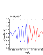
Figure 4: (Color online) The LDOS as a function of distance from the line defect along $y$ or $x$ axis at zero bias voltage.

Correspondingly, the LDOS in this case is

$$\rho_{I,II}(y,\omega)=\sum_{k_{x},k_{y}>0,s}|\psi_{I,II}^{s}(x,y;{\bf k})|^{2}\delta(\omega-E_{{\bf k}s}).$$

According to Eq. (15) and using the parameters in Bi₂Te₃, we also calculate the LDOS near the SD along $x$ axis at different bias voltages and strengths of the $\delta$ potential, shown in Fig. 3. We can see that the amplitude of the LDOS modulation also changes with $U_{0}$ and $\omega$. When $\omega$ is fixed, the period and the phase of the oscillations are also independent of $U_{0}$. However, on the points symmetrical about the SD, the LDOS at $\omega=100$ meV has the same oscillatory features with that induced by the SD along $y$ axis. In contrast, when $\omega=-120$ meV, the LDOS has two maximum or minimum values. We note that $T_{x}(100)\approx 33.0$ Åand $T_{x}(-120)\approx 74.0$ Å. The oscillatory characteristics are also produced by quasiparticle interference between two points on the constant-energy contours in Fig. 2, similar to the previous case. We find that $T_{x}(100)\sim\frac{2\pi}{|{\bf q}_{B}-{\bf q}_{C}|}=\frac{2\pi}{|{\bf q}_{A}-{\bf q}_{D}|}=\frac{\pi}{0.0952}=33.0$ Åwhile $T_{x}(-120)\sim\frac{2\pi}{|{\bf q}_{F}-{\bf q}_{G}|}=\frac{2\pi}{|{\bf q}_{E}-{\bf q}_{H}|}=\frac{\pi}{0.0419}=74.98$ Å. With increasing $\omega$, $|{\bf q}_{B}-{\bf q}_{C}|$ and $|{\bf q}_{F}-{\bf q}_{G}|$ become longer, and so the periods of the oscillations become smaller. When $\omega$ decreases to the values near the Dirac point, the quasiparticle interference associated with the wave vector ${\bf q}_{E}-{\bf q}_{H}$ or ${\bf q}_{F}-{\bf q}_{G}$ becomes very weaker and the periods of the oscillations become very larger. Therefore, the LDOS is almost constant. These results are consistent with the STM observations [10,11].

Because the modulation wave vector at $\omega=100$ meV is different from that at $\omega=-120$ meV, it is expected that the two modulation wave vectors compete at small energies. Fig. 4 shows the LDOS at zero bias voltage for the two kinds of SDs. Obviously, the LDOS modulations cannot be fitted by a wave vector connecting two points on the Fermi surface [10].

In summary, we have investigated the impact of the SD along $x$ or $y$ axis on the surface states of topological insulators. We discover for the first time that there are spin rotations when the topological surface states move through the $\delta$ potential barrier. The oscillations of the LDOS near the SDs are induced by quasiparticle interference. This agrees qualitatively with the STM experiments. The period and phase of the oscillations are independent of the strength of SDs at high positive or negative bias voltage. But the amplitudes of the oscillations are sensitive to the strength of SDs and the bias voltages. We also find that the oscillations of the LDOS at high energies induced by the SD along $y$ or $x$ axis are associated with the same points on the constant-energy contours. Therefore, their periods have special relations, i.e. $T_{y}(|\omega|)=\sqrt{3}T_{x}(|\omega|)$ and $T_{y}(-|\omega|)=\frac{1}{\sqrt{3}}T_{x}(-|\omega|)$, where $\omega$ is large. We hope that such relations could be verified by future STM experiments.

This work was supported by the Texas Center for Superconductivity at the University of Houston and by the Robert A. Welch Foundation under the Grant no. E-1411.

References

(1) Xiao-Liang Qi and Shou-Cheng Zhang, Phys. Today, 63, 33 (2010); Rev. Mod. Phys. (in press).
(2) M. Z. Hasan and C. L. Kane, Rev. Mod. Phys. 82, 3045 (2010).
(3) D. Hsieh et al, Science 323, 919 (2009).
(4) Y. Xia et al, Nature Phys. 5, 398 (2009).
(5) H. Zhang et al, Nature Phys. 5, 438 (2009).
(6) Y.L. Chen et al, Science 325, 178 (2009).
(7) Y.L. Chen et al, Phys. Rev. Lett. 104, 016401 (2010).
(8) Liang Fu, Phys. Rev. Lett. 105, 266401 (2010).
(9) T. Zhang et al, Phys. Rev. Lett. 103, 266803 (2009).
(10) Z. Alpichshev et al, Phys. Rev. Lett. 104, 016401 (2010).
(11) K. K. Gomes et al, arXiv:0909.0921 (unpublished).
(12) J. Seo et al, Nature (London) 466, 343 (2010).
(13) M.F. Crommie, C. P. Lutz, and D. M. Eigler, Nature 363, 524 (1993).
(14) L. C. Davis et al, Phys. Rev. B 43, 3821 (1991).
(15) R. R. Biswas and A. V. Balatsky, Phys. Rev. B 83, 075439 (2011).