Synthetic observations of simulated pillars of creation

Abstract

We present synthetic observations of star-forming interstellar medium structures obtained by hydrodynamic calculations of a turbulent box under the influence of an ionising radiation field. The morphological appearance of the pillar-like structures in optical emission lines is found to be very similar to observations of nearby star forming regions. We calculate line profiles as a function of position along the pillars for collisionally excited [OIII]$\lambda$5007, [NII]$\lambda$6584 and [SII]$\lambda$6717, which show typical FWHM of 2–4 km s^-1 km/s. Spatially resolved emission line diagnostic diagrams are also presented which show values in general agreement with observations of similar regions. The diagrams, however, also highlight significant spatial variations in the line ratios, including values that would be classically interpreted as shocked regions based on one-dimensional photoionisation calculations. These values tend to be instead the result of lines of sight intersecting which intersect for large portions of their lenghts the ionised–to–neutral transition regions in the gas. We caution therefore against a straightforward application of classical diagnostic diagrams and one–dimensional photoionisation calculations to spatially resolved observations of complex three-dimensional star forming regions.

1 Introduction

The influence of stellar feedback on the star formation process itself is one of the most important issues in this field of astrophysics. Feedback from OB–type stars, in the form of photoionizing radiation, radiation pressure, winds, and supernovae, can be both positive (i.e. enhancing or hindering the star formation efficiency) and negative and may be responsible for regulating the efficiency and rate of star formation on the scale of giant molecular clouds (GMCs).
The destructive effects of feedback, in the sense of quenching star formation, gas–expulsion and dispersal of young clusters, have been studied by many authors. The dynamical influence of gas expulsion on clusters has been examined by, e.g., Hills (1980), Goodwin (1997), Boilly & Kroupa (2003,a,b) Goodwin & Bastian (2006), while self–regulation of star formation by limiting the star formation efficiency has been modelled by, e.g., Whitworth (1979), Bodenheimer et al. (1979), Tenorio–Tagle & Bodenheimer (1988), Franco et al. (1994), Matzner et al. (2002).
Conversely, numerous authors have studied the positive effects of feedback in the context of induced or triggered star formation, partly spurred on by a recent crop of exquisite observations of triggering apparently in progress. The popular collect–and–collapse model of triggering has been studied analytically and numerically many times (e.g. Whitworth et al., 1994, Wünsch & Palouš, 2001, Dale et al., 2007a) and has been observed in action (e.g. Zavagno et al, 2006, Deharveng et al., 2008, Zavagno et al., 2010). However, for this model to be valid, it is necessary to assume that the gas on which feedback is acting is relatively smooth and quiescent, conditions which are not always met, especially not in the inner regions of turbulent GMCs where the density and velocity fields in the gas are highly inhomogeneous. Under these conditions, it is very difficult to devise an analytic description of the effects of feedback.
This question has instead been approached numerically by means of hydrodynamical simulations modified to include the thermal effect of photoionisation. The complexity of such simulations and the inevitable dependence of the results on the chosen initial conditions demand strict comparisons with observations before meaningful conclusions may be drawn. One such test for how realistic these models are involves running large-scale cluster simulations and computing statistics for (e.g.) the initial mass function (IMF) of the stars and their multiplicity. Such statistics, however, are often difficult to obtain with the required accuracy. The stellar IMF is a steep function and at least several hundred stars are required to adequately sample it over a meaningful range of masses. Combined with the difficulty of modelling feedback itself, this problem requires large and time–consuming calculations ( Klessen, Krumholz & Heitsch 2009; Dale and Bonnell, 2011, submitted).
Another approach is to compare the morphology of structures in the interstellar medium (ISM) that are influenced by the effects of photoionising radiation. Spatially resolved imaging (e.g. from the Hubble Space Telescope) and spectroscopy of young star forming regions (e.g. Hester et al. 1996; Pound et al. 2003; Gahm et al. 2006; Matsuura et al. 2007; Smith et al. 2010; Westmoquette et al. 2010), provide a wealth of crucial information and hold the promise of helping to constrain models of ISM evolution. Until now, the problem of realistically computing the observable radiation fields from systems produced by hydrodynamical calculations has only been moderately explored (Arthur et al 2001). The main reason for this is that the majority of hydrodynamical codes only include the thermal effects of photoionisation in a very approximate fashion (see Ercolano & Gritschneder, 2011a; Dale et al 2007b), preventing the calculation of the detailed thermal and ionisation structure of the gas required for the prediction of emission line and continuum radiation from the region. A solution to this problem is to employ a dedicated three-dimensional photoionisation code as a postprocessing step to analyse the emission from density snapshots of the hydrodynamical calculations.

We use this approach in this paper to explore the observational appearance of the star-forming pillars obtained by the recent calculations of Ercolano & Gritschneder (2011b, EG11), which modelled the impact of radiation from high–mass stars on the turbulent ISM. The calculations improved upon the previous work of Gritschneder et al. (2009b, 2010) by including the effects of diffuse ionizing radiation fields on the hydrodynamics and thus on the shaping of the ISM and the formation of pillar-like structure. EG11 found that the diffuse fields promote the detachment of dense clumps and filaments from the parent cloud, and produce denser and more spatially confined structures. In this paper we wish to investigate the observational appearance of such structures in optical emission, to verify the morphological similarity to observations, and to explore the potential of spatially resolved line ratio diagnostics.

We describe our numerical methods in Section 2 and main results in Section 3. Section 4 contains a brief summary and conclusions.

2 Numerical Methods

2.1 Hydrodynamical calculations

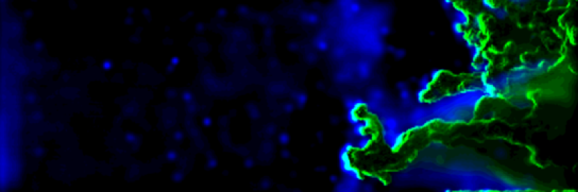
Figure 1: False colour composite image of the EG11 pillar at t = 500kyr, where red is H$\alpha$, blue is [OIII]$\lambda\lambda$5007,4959 and green is a combination of the two lines.

The hydrodynamic simulations were performed with the tree-SPH/ionisation code iVINE (Gritschneder et al 2009a). iVINE treats the ionisation of the turbulent ISM under the assumption of plane-parallel irradiation on the computational domain. The surface facing the ionising source is decomposed into equally–spaced bins, whose size is chosen according to the smoothing length of the particles there. The bins or rays are subsequently refined as the radiation penetrates the gas according to the local smoothing length. Along these rays the optical depth is calculated and a new pressure is assigned to each particle $i$ according to:

$$P_{\mathrm{i}}=\left(\frac{T_{\mathrm{hot}}\eta_{\mathrm{i}}}{\mu_{\mathrm{hot}}}+\frac{T_{\mathrm{cold}}(1-\eta_{\mathrm{i}})}{\mu_{\mathrm{cold}}}\right)\frac{k_{\mathrm{B}}\rho_{\mathrm{i}}}{m_{\mathrm{p}}}.$$ (1)

Here, $\eta$ is the ionisation degree, defined as the ratio of the number density of free electrons to the total number of hydrogen nuclei, $T_{hot}=10^{4}K$, $T_{cold}=10K$, $\mu_{\mathrm{hot}}=0.5$ and $\mu_{\mathrm{cold}}=1.0$ are the temperatures and the mean molecular weights of the ionised and neutral gas in the case of pure hydrogen, respectively. $k_{\mathrm{B}}$ is the Boltzmann constant, $m_{\mathrm{p}}$ is the proton mass and $\rho_{\mathrm{i}}$ is the density of the SPH particle.

In the results presented here, the diffuse ionisation is included according to EG11. The shadowed particles with a density lower than $n=100cm^{-3}$ are assigned a new, higher temperature according to a fitted function. This function is derived from comparisons of previous simulations with full 3D postprocessing using the mocassin code (Ercolano et al. 2003, 2005, 2008). The cold, dense, neutral gas is kept at a temperature of $T_{cold}=10K$ under the assumption that it can cool fast enough, i.e. it is treated as isothermal.

Hydrodynamic and gravitational forces are then calculated for the particles with the accuracy parameters given in (Gritschneder 2009b). The initial density and velocity distribution mimics the turbulent ISM at Mach 5 inside a computational domain of $4pc^{3}$ with a mean density of $n=300cm^{-3}$. To create synthetic observations of the resulting structures discussed in EG11, we take a subdomain starting from the irradiated surface at the $y$=0 plane and spanning $3pc$ in the $y$-direction and $1pc$ in the $x$- and $z$-directions around the most prominent features of the simulations in EG11. We map the hydrodynamic quantities in this region on an equally–spaced grid ($384\times 128^{2}$). With this data we perform the postprocessing with mocassin described below.

2.2 Photoionisation calculations

We used the 3D photoionisation code mocassin (Ercolano et al. 2003, 2005, 2008) to compute the detailed ionisation and temperature structure from the 5kyr snapshot of the above–described region containing the main pillar in the EG11 simulation. The code uses a Monte Carlo approach to the transfer of radiation, allowing the treatment of both the direct stellar radiation and the diffuse fields for arbitrary geometries and density distributions. The gas is heated mainly by photoionisation of hydrogen and other abundant elements. Cooling is dominated by collisionally excited lines of heavy elements, but contributions from recombination lines, free-bound, free-free and two-photon continuum emission are also included. We have assumed typical HII region abundances for the gas phase, namely (given as number densities with respect to hydrogen): He/H = 0.1, C/H = 2.2e-4, N/H = 4.0e-5, O/H = 3.3e-4, Ne/H = 5.0e-5, S/H = 9.0e-6.

Emission lines produced in each volume element are then computed by solving the statistical equilibrium problem for each atom and ion at the local temperature and ionisation conditions. The atomic database includes opacity data from Verner et al. (1993) and Verner & Yakovlev (1995), energy levels, collision strengths and transition probabilities from Version 5.2 of the CHIANTI database (Landi et al. 2006, and references therein) and the hydrogen and helium free-bound continuous emission data of Ercolano & Storey (2006).

The current version of the code can treat the atomic and ionised gas phases and dust, but no chemical network is currently included, preventing the calculation of physical conditions and emission from photodissociation or molecular regions (but see Bisbas et al 2011 for recent developments in this area).

2.3 Visualisation Tool

The 3D grids of temperature, ionisation structure and emission from mocassin were further post-processed by means of our newly–developed, Python-based suite of tools, which will shortly be made freely available to the community on the mocassin website (www.3d-mocassin.net). The tools provide 2D projections of the grids along the three major axes, accounting for dust extinction along the line of sight. Velocity maps, line profiles and emission line diagnostic diagrams, like those presented in Section 3 of this paper, are also available. The new software will be distributed with an online manual, where further details on the available routines will be provided.

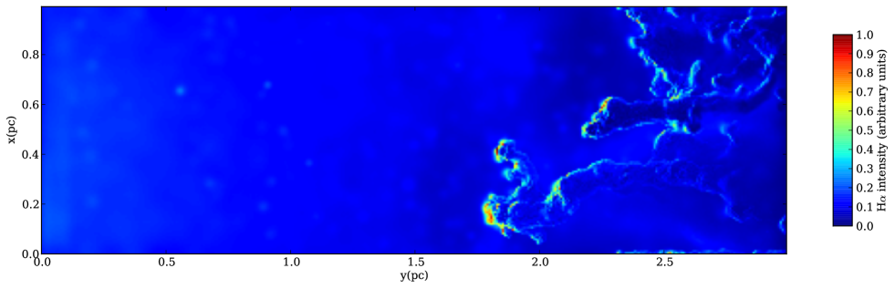
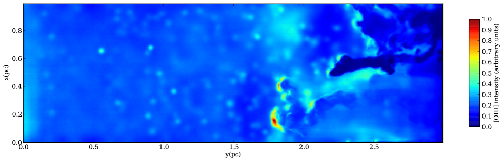
Figure 2: Top Panel: H$\alpha$ image of the EG11 pillar at t = 500kyr. Bottom Panel: same image in [OIII]$\lambda\lambda$5007,4959.

3 Results

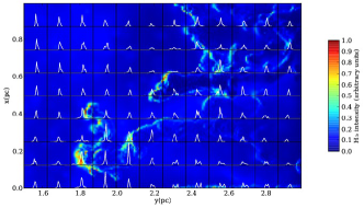
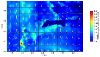
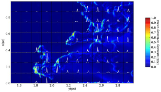
Figure 3: Predicted profiles for H$\alpha$ (top right), [OIII]$\lambda$5007 (top left), [NII]$\lambda$6584 (bottom left) and [SII]$\lambda$6717 (bottom right) are shown. The width of each box is 30 km s^-1 (centred on zero) and the emissivities are in arbitrary units, normalised to the brightest line.

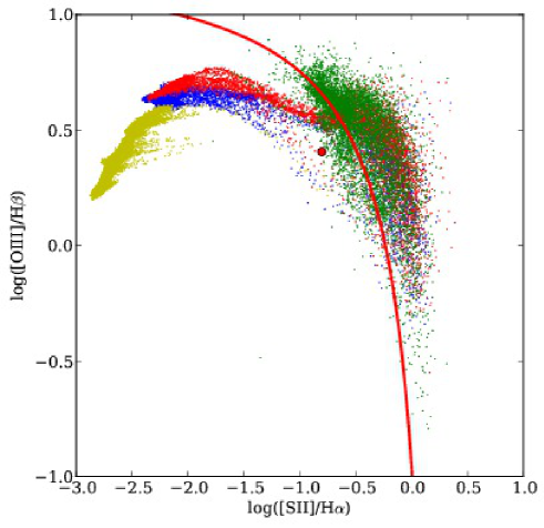
Figure 4: [OIII]/H$\beta$ versus [SII]/H$\alpha$ at each pixel on the 2D projected images. The integrated value for all pixels is shown as the red point on the figures. The solid red line represents the Kewley et al (2001) line separating star–forming galaxies from AGN. The points are colour-coded according to distance from the left-hand side of the simulation box. The green points are for $y$ $>$ 2.6pc, red for 2.6pc $>$ $y$ $>$ 2.2pc, blue for 2.2pc $>$ $y$ $>$ 1.8pc and yellow for $y$ $<$ 1.8pc.

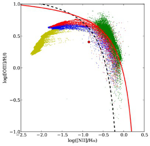
Figure 5: [OIII]/H$\beta$ versus [NII]/H$\alpha$ at each pixel on the 2D projected images. The integrated value for all pixels is shown as the red point on the figures. The solid red line represents the Kewley et al (2006) line separating star–forming galaxies from AGN, while the dashed line shows the line from Kauffmann et al 2003 separating pure–star–forming galaxies from composite star–forming/AGN systems. The points are colour-coded according to distance from the left-hand side of the simulation box. The green points are for $y$ $>$ 2.6pc, red for 2.6pc $>$ $y$ $>$ 2.2pc, blue for 2.2pc $>$ $y$ $>$ 1.8pc and yellow for $y$ $<$ 1.8pc.

3.1 Morphology

EG11 concluded that one of the effects of diffuse fields in the simulation of pillar formation was that the structures obtained were denser, spatially thinner and that they would eventually detach from the parent turbulent cloud. The famous HST images of e.g. the Pillars of Creation in the Eagle nebula show, however, structures that are apparently coherent. We constructed 2D projected intensity maps of optical emission lines from the 500kyr snapshot of the EG11 simulations to verify that the apparent morphological constraint provided by the HST image of coherent pillars is still respected. Figure 1 shows a combined false colour composite image of the EG11 pillar at t = 500kyr, where red is H$\alpha$, blue is [OIII]$\lambda\lambda$5007,4959 and green is a combination of the two channels. The top and bottom panels of Figure 2 show the same region in the individual channels, respectively H$\alpha$ and [OIII]$\lambda\lambda$5007,4959. All images account for dust extinction along the line of sight, for the length of the simulation box, according to the interstellar extinction curve of Weingartner & Draine (2001) for a Milky Way grain size distribution for RV =3.1, with C/H = bC = 60 ppm in log-normal size distributions, but renormalised by a factor 0.93. This grain model is considered to be appropriate for the typical diffuse HI cloud in the Milky Way.

The figure clearly shows that the line of sight integrals of emission lines from the ionised gas at the surface of the pillars, give the desired appearance of internally coherent structures. The spatial thickness of such structure is of the order of a tenth of a parsec, which is consistent with observations.

3.2 Line profiles

The gas velocity information combined with the emission measure at each volume element allows us to compute predicted emission line profiles along the structures. This is shown in Figure 3 where the predicted profiles for H$\alpha$ (top right), [OIII]$\lambda$5007 (top left), [NII]$\lambda$6584 (bottom left) and [SII]$\lambda$6717 (bottom right) are shown. The width of each box is 30 km s^-1 (centred on zero) and the emissivities are in arbitrary units, normalised across the regions to the brightest lines. Typical FWHM for the profiles are 2–4 km s^-1. It is useful to note at this point that Westmoquette et al (2009) report the presence of both a narrow ($\sim$20km/s) and a broad ($50-150$km/s) component in the H$\alpha$ line profiles from their optical/near-IR IFU observations of a gas pillar in the Galactic HII region NGC 6357, which contains the young open star cluster Pismis 24. They interpret the broad component as being formed in ionized gas within turbulent mixing layers on the pillar’s surface, generated by the shear flows of the winds from the O stars in the cluster. Our simulations do not include stellar winds and are instead influenced only by the thermal pressure of the hot ionised gas. Relative gas velocities therefore cannot exceed a few times the speed of sound in the ionised gas, approximately 10km s^-1, which explains why we only can reproduce the narrow component of the emission lines.

3.3 Line Ratio Diagnostics

Emission line ratios are often used as diagnostics of gas properties such as temperature and density, and sometimes also to distinguish between shock– and photo–ionisation in the gas. The development of diagnostic tools dates back to more than forty years ago when one-dimensional photoionisation models started being developed (e.g. Harrington 1968). Diagnostic diagrams were successively developed, based on grids of 1D photoionisation models, often calibrated with empirical data from spatially unresolved observations. Some of the most widely used diagnostic diagrams are the so-called BPT diagrams (Baldwin, Phillips & Terlevich 1981), which consist of comparing the ratios of strong collisionally excited lines (e.g. [OIII]$\lambda\lambda$5007,4959, [NII]$\lambda$6583, 48, [SII]$\lambda$6717,31) to the main hydrogen recombination lines (e.g. H$\beta$, H$\alpha$). The excitation and ionisation parameter in a given region can be determined by comparison of different ionised species or of lines with different temperature dependences. Calibration of models with observations has allowed regions in such plots where the line ratios are dominated by photoionisation over shocks to be distinguished, and the determination of the nature of astronomical objects, e.g. HII regions, active galactic nuclei, by comparison of their diagnostic spectra with model predictions (Kewley et al 2001, Kauffmann et al 2003, Kewley et al 2006).

It is important to note, however, that such diagnostic tools were developed for spatially unresolved observations where the integrated emission from the whole galaxy or nebula was contained in a given emission line ratio. More recently the same tools have been applied for the interpretation of spatially resolved observations, e.g. IFU observations of extended HII regions (García-Benito et al. 2010, Monreal-Ibero et al 2011, Relano et al 2010). This approach has to be taken with caution, given that a line of sight projection of a complex 3D structure, which contains fully ionised as well as neutral regions, is not directly comparable with the results from a radiation bound 1D (slab or spherically symmetric) photoionisation model. Indeed a 2D projection of a 3D cloud will show pixel-to-pixel variations of the line ratios corresponding to the local gas conditions along the line of sight.

This is shown in Figures 4 and 5 where each pixel on the 2D projections of our pillars is plotted on typical BPT diagrams. The integrated value for all pixels is shown as the red point on the figures. The solid red line shown separates the area of the BPT diagrams that is traditionally considered to be occupied by HII regions dominated by photoionisation (below the line) from that occupied by AGNs dominated by shock-ionisation (Kewley et al 2001, Kewley et al 2006). The dashed line in Figure 5 is taken from Kauffmann et al 2003 and represents a stricter partition of the diagram in that it divides pure star–forming regions (below the line) from composite objects such as Seyfert–HII galaxies whose spectra exhibit strong contributio¡ns from star formation and AGN. The points are colour-coded by distance from the left-hand side of the simulation box on which the stellar radiation field impinges. In particular the green points are for $y$ $>$ 2.6pc, red for 2.6pc $>$ $y$ $>$ 2.2pc, blue for 2.2pc $>$ $y$ $>$ 1.8pc and yellow for $y$ $<$ 1.8pc. The majority of the points lie, as expected, in the photoionisation region of the diagram. However, in Figure 4 4$\%$ and in Figure 5 16$\%$ of the points lie well beyond the red line, apparently suggesting that shocks may be responsible for the observed line ratios. This is of course not the case in our simulations and the observed values are simply due to the complex 3D distribution of the gas, whereby the lines of sight at these large $y$-positions intersect regions of neutral or quasi-neutral gas. In the ionised–to–neutral transition regions, singly ionised N and S are relatively more abundant than in the region where hydrogen is fully ionised (the ionisation potential for N⁰ is 14.5eV and that for S$0$ is 10.3eV), pushing the line ratios to the right of the diagrams. The message to be taken away from these figures is that care should be taken when interpreting spatially resolved observations using diagnostic diagrams or 1D photoionisation calculations, which may lead to incorrect conclusions with regard to spatial variations of abundances and/or the ionisation mechanism (see also e.g. O’Dell et al 2011 versus Wood et al 2011, or see Balick et al 1994 versus Goncalves et al 2006).

4 Conclusions

We have presented synthetic observations of optical emission lines from complex density and velocity fields obtained by the three-dimensional smooth particle hydrodynamics simulations of Ercolano & Gritschneder (2011). These calculations consist of a turbulent box irradiated by a plane-parallel ionising field, and present at 500kyr density structures reminiscent of nearby star-forming regions (e.g. the Pillars of Creation, the Horse Head Nebula). We have performed three-dimensional radiative transfer and photoionisation calculations and produced emission line maps in typical ionised gas tracers, including H$\beta$, [OIII]$\lambda$5007, [NII]$\lambda$6584 and [SII]$\lambda$6717 The resulting composite three-colour images that we obtained are directly comparable with, e.g., images from the Hubble Space Telescope (Hester et al. 1996). The morphological appearance of our synthetic pillar images is in good agreement with the observations. We have also produced spatially resolved emission line profiles, which show typical FWHM of 2–4 km s^-1 km s^-1 and dispersions of 30 km s^-1, in agreement with photoionised gas with sound-speeds of approximately 10 km s^-1.

Finally we have studied the spatial variation of emission line diagnostics by means of classical BPT diagrams. The volume-averaged diagnostics are consistent with the loci expected for photoionised gas, however we show that significant location-dependent variations of the diagnostic values are to be expected, due to the complex three-dimensional ionisation, excitation and temperature distributions along the different lines of sight. In particular we draw attention to a number of surface elements that show diagnostics consistent with gas that is shock-ionised, rather than photoionised, according to the classical interpretation of the BPT diagrams by means of one-dimensional photoionisation calculations (e.g. Kewley et al 2006). The gas in this regions however is not shocked, and the altered diagnostic values are only a result of lines of sight that intercept large portions of the ionised to neutral transition regions in the box. We therefore conclude that the straightforward application of diagnostic diagrams based on one-dimensional photoionisation calculations is not suitable to the interpretation of spatially resolved observations of complex star-forming regions.

5 Acknowledgements

We thank the anonymous referee for a constructive report which helped us to make the paper clearer. M.G. acknowledges funding by the China National Postdoc Fund Grant No. 20100470108 and the National Science Foundation of China Grant No. 11003001.

References

- [] Arthur, S. J., Henney, W. J., Mellema, G., de Colle, F., & Vazquez-Semadeni, E. 2011, MNRAS, 414, 1747
- [Baldwin et al.(1981)] Baldwin, J. A., Phillips, M. M., & Terlevich, R. 1981, PASP, 93, 5
- [Balick et al.(1994)] Balick, B., Perinotto, M., Maccioni, A., Terzian, Y., & Hajian, A. 1994, ApJ, 424, 800
- [Bastian & Goodwin(2006)] Bastian, N., & Goodwin, S. P. 2006, MNRAS, 369, L9
- [Bisbas et al.(2011)] Bisbas, T. G., Bell, T. A., Viti, S., Yates, J., Barlow, M., & Ercolano, B. 2011, IAU Symposium, 280, 98P
- [Bodenheimer et al.(1979)] Bodenheimer, P., Tenorio-Tagle, G., & Yorke, H. W. 1979, ApJ, 233, 85
- [Boily & Kroupa(2003)] Boily, C. M., & Kroupa, P. 2003, MNRAS, 338, 665
- [Boily & Kroupa(2003)] Boily, C. M., & Kroupa, P. 2003, MNRAS, 338, 673
- [Dale et al.(2007)] Dale, J. E., Bonnell, I. A., & Whitworth, A. P. 2007a, MNRAS, 375, 1291
- [Dale et al.(2007)] Dale, J. E., Ercolano, B., & Clarke, C. J. 2007b, MNRAS, 382, 1759
- [Deharveng et al.(2008)] Deharveng, L., Lefloch, B., Kurtz, S., Nadeau, D., Pomarès, M., Caplan, J., & Zavagno, A. 2008, A&A, 482, 585
- [Ercolano et al.(2003)] Ercolano, B., Barlow, M. J., Storey, P. J., & Liu, X.-W. 2003, MNRAS, 340, 1136
- [Ercolano & Gritschneder(2011a)] Ercolano, B., & Gritschneder, M. 2011a, IAU Symposium, 270, 301
- [Ercolano & Gritschneder(2011b)] Ercolano, B., & Gritschneder, M. 2011b, MNRAS, 413, 401
- [Ercolano et al.(2005)] Ercolano, B., Barlow,M. J., & Storey, P. J. 2005, MNRAS, 362, 1038
- [Ercolano & Storey(2006)] Ercolano, B., & Storey, P. J. 2006, MNRAS, 372, 1875
- [Ercolano et al.(2008a)] Ercolano, B., Young, P. R., Drake, J. J., & Raymond, J. C. 2008, ApJS, 175, 5345, 165
- [Franco et al.(1994)] Franco, J., Shore, S. N., & Tenorio-Tagle, G. 1994, ApJ, 436, 795
- [Gahm et al. (2006)] Gahm G. F., Carlqvist P., Johansson L. E. B., Nikolić S., 2006, A&A, 454, 201
- [García-Benito et al.(2010)] García-Benito, R., et al. 2010, MNRAS, 408, 2234
- [Gonçalves et al.(2006)] Gonçalves, D. R., Ercolano, B., Carnero, A., Mampaso, A., & Corradi, R. L. M. 2006, MNRAS, 365, 1039
- [Goodwin(1997)] Goodwin, S. P. 1997, MNRAS, 286, 669
- [Gritschneder et al.(2009)] Gritschneder, M., Naab, T., Burkert, A., Walch, S., Heitsch, F., & Wetzstein, M. 2009a, MNRAS, 393, 21
- [Gritschneder et al.(2009)] Gritschneder, M., Naab, T., Walch, S., Burkert, A., & Heitsch, F. 2009b, ApJL, 694, L26
- [Gritschneder et al.(2010)] Gritschneder, M., Burkert, A., Naab, T., & Walch, S. 2010, ApJ, 723, 971
- [Harrington(1968)] Harrington, J. P. 1968, ApJ, 152, 943
- [Hester et al. (1996)] Hester J. J., et al., 1996, AJ, 111, 2349
- [Hills(1980)] Hills, J. G. 1980, ApJ, 235, 986
- [Kewley et al.(2006)] Kewley, L. J., Groves, B., Kauffmann, G., & Heckman, T. 2006, MNRAS, 372, 961
- [Klessen et al.(2009)] Klessen, R. S., Krumholz, M. R., & Heitsch, F. 2009, arXiv:0906.4452
- [Landi et al.(2006)] Landi, E., Del Zanna, G., Young, P. R., Dere, K. P., Mason, H. E., & Landini, M. 2006, ApJS, 162, 261
- [Matzner(2002)] Matzner, C. D. 2002, ApJ, 566, 302
- [Matsuura et al. (2007)] Matsuura M., et al., 2007, MNRAS, 382, 1447
- [Monreal-Ibero et al.(2011)] Monreal-Ibero, A., Relaño, M., Kehrig, C., Pérez-Montero, E., Vílchez, J. M., Kelz, A., Roth, M. M., & Streicher, O. 2011, MNRAS, 413, 2242
- [O’Dell et al.(2011)] O’Dell, C. R., Ferland, G. J., Porter, R. L., & van Hoof, P. A. M. 2011, ApJ, 733, 9
- [Pound et al. (2003)] Pound, M. W., Reipurth, B., & Bally, J. 2003, AJ, 125, 2108
- [Relaño et al.(2010)] Relaño, M., Monreal-Ibero, A., Vílchez, J. M., & Kennicutt, R. C. 2010, MNRAS, 402, 1635
- [Smith et al. (2010)] Smith, N., Bally, J., & Walborn, N. R. 2010, MNRAS, 405, 1153
- [Tenorio-Tagle & Bodenheimer(1988)] Tenorio-Tagle, G., & Bodenheimer, P. 1988, ARA&A, 26, 145
- [Weingartner & Draine(2001)] Weingartner, J. C., & Draine, B. T. 2001, ApJ, 548, 296
- [Westmoquette et al. (2010)] Westmoquette M. S., Slavin J. D., Smith L. J., Gallagher J. S., III, 2010, MNRAS, 402, 152
- [Whitworth(1979)] Whitworth, A. 1979, MNRAS, 186, 59
- [Whitworth et al.(1994)] Whitworth, A. P., Bhattal, A. S., Chapman, S. J., Disney, M. J., & Turner, J. A. 1994, A&A, 290, 421
- [Wünsch & Palouš(2001)] Wünsch, R., & Palouš, J. 2001, A&A, 374, 746
- [Zavagno et al.(2006)] Zavagno, A., Deharveng, L., Comerón, F., Brand, J., Massi, F., Caplan, J., & Russeil, D. 2006, A&A, 446, 171
- [Zavagno et al.(2010)] Zavagno, A., et al. 2010, A&A, 518, L81