Random Matrix Models for Dirac Operators at finite Lattice Spacing

Abstract:

We study discretization effects of the Wilson and staggered Dirac operator with $N_{\rm c}>2$ using chiral random matrix theory (chRMT). We obtain analytical results for the joint probability density of Wilson-chRMT in terms of a determinantal expression over complex pairs of eigenvalues, and real eigenvalues corresponding to eigenvectors of positive or negative chirality as well as for the eigenvalue densities. The explicit dependence on the lattice spacing can be readily read off from our results which are compared to numerical simulations of Wilson-chRMT. For the staggered Dirac operator we have studied random matrices modeling the transition from non-degenerate eigenvalues at non-zero lattice spacing to degenerate ones in the continuum limit.

1 Introduction

Chiral RMT is a powerful mathematical tool to calculate eigenvalue correlations in the infrared limit of quantum chromodynamics (QCD) and has been successfully applied to Dirac spectra for almost two decades [1]. In the low energy limit QCD exhibits universal behavior that agrees with chRMT with the same symmetries as the Dirac operator. In the continuum limit as well as for finite lattice spacing, $a\neq 0$, random matrix ensembles have been constructed that reproduce the eigenvalue correlations of the lattice QCD Dirac operator.

Discretization effects of the Wilson Dirac operator were already studied with the help of chiral perturbation theory in the $p$-limit [2, 3, 4]. Furthermore it was shown that the chiral Lagrangian agrees with Wilson chRMT in this limit [5, 6, 7]. Random matrix theory enables us to get results which were not accessible before. We derive the joint probability density (jpd) of the non-Hermitian version for the random matrix ensemble proposed in Ref. [5] and present its eigenvalue densities in the microscopic limit which have to agree with the low lying eigenvalues of the Wilson Dirac operator. In our representation we are able to distinguish between the eigenvalue densities of the complex eigenvalues and of the real eigenvalues with eigenvectors of positive and negative chirality.

Staggered fermions are widely used in lattice simulations mainly because of their low computational costs. We study a matrix model that reproduces the single trace terms in the chiral Lagrangian (reduced to staggered fermions in two dimensions) incorporating taste breaking effects at order $a^{2}$ [16]. It is the model proposed in Ref. [15] for staggered fermions in two dimensions which we expect to be analytically solvable.

In Sec. 2, we consider the Wilson-chRMT [5] and study its spectral properties. A random matrix ensemble for the staggered fermions is proposed in Sec. 3.

2 Wilson fermions

Wilson-chRMT.

The ensemble introduced in Ref. [5] is

$$D_{\rm W} = \left(\begin{array}[]{cc}aA&W\\ -W^{\dagger}&aB\end{array}\right)\quad{\rm distributed\ by}\quad P(D_{\rm W})\propto\exp\left[-\frac{n}{2}(\textrm{tr}A^{2}+\textrm{tr}B^{2})-n\textrm{tr}WW^{\dagger}\right].$$ (3)

For $a=0$ this gives the chiral Gaussian unitary ensemble (chGUE) that describes the infrared Dirac spectrum of continuum QCD [1]. The complex $n\times(n+\nu)$ matrices $W$ and $W^{\dagger}$ preserve chiral symmetry, whereas the Hermitian matrices $A$ and $B$ break the chiral symmetry and are identified with the Wilson term. In the microscopic limit ($n\to\infty$) the rescaled lattice spacing $\widehat{a}^{2}=na^{2}/2$, the rescaled eigenvalues $\widehat{z}=2nz$ as well as the index of the Dirac operator $\nu$ are kept fix. Then, spectral correlations of Wilson-chRMT become universal and agree with infrared Wilson chiral perturbation theory ($\chi$PT) [6, 7]. The volume of space-time $V$ is identified with the matrix dimension $n$.

Let $\widetilde{a}$ be the physical lattice spacing. Then, the relation to the rescaled quantity is $\widehat{a}=\sqrt{W_{8}V}\widetilde{a}$. The low energy constants $W_{6}$ and $W_{7}$ corresponding to the squares of traces in the action of the Goldstone bosons [5, 6] are suppressed in the large $N_{\rm c}$ limit [8] and will not be considered here. We are interested in the quenched case and a more general setting will be considered elsewhere.

Without loss of generality, let $\nu\geq 0$. Due to the $\gamma_{5}=\textrm{diag}(\leavevmode\hbox{\small 1\kern-3.8pt\normalsize 1}_{n},-\leavevmode\hbox{\small 1\kern-3.8pt\normalsize 1}_{n+\nu})$-Hermiticity of $D_{\rm W}$ ($(\gamma_{5}D_{\rm W})^{\dagger}=\gamma_{5}D_{\rm W}$), the eigenvalues are either real or come in complex conjugated pairs. There are $\nu$ generic real eigenvalues corresponding to the $\nu$ zero modes at $a=0$. Moreover, $2l$ ($0\leq l\leq n$) additional real modes may appear when $l$ complex conjugated eigenvalue pairs enter the real axis.

Often the Hermitian version of the Wilson Dirac operator $D_{5}=\gamma_{5}D_{\rm W}$ is studied because it simplifies lattice simulations [10] as well as RMT calculations [5, 6, 7, 9]. However, only $D_{\rm W}$ is directly related to the chiral symmetry breaking which is our main motivation for studying the non-Hermitian version.

The joint probability distribution.

Analogously to Hermitian matrices, the $\gamma_{5}$ Hermiticity allows us to quasi-diagonalize the matrix $D_{\rm W}$ by a non-compact unitary matrix $U\in\textrm{U}(n,n+\nu)$,

$$D_{\rm W}=UX^{(l)}U^{-1}\ \textrm{and}\ X^{(l)}=\textrm{diag}\left[x_{1},\left(\begin{array}[]{cc}x_{2}&y_{2}\\ -y_{2}&x_{2}\end{array}\right),x_{3}\right].$$ (6)

The real matrices $x_{1}$, $x_{2}$, $y_{2}$ and $x_{3}$ are diagonal with dimensions $l$, $n-l$, $n-l$ and $l+\nu$, respectively. The ensemble decomposes in $n+1$ disjoint sets differing in the number of complex conjugate pairs, $n-l$, or equivalently, in the number of real modes, $2l+\nu$. The $l$ complex pairs are given by $(z_{2},z^{*}_{2})=(x_{2}+\imath y_{2},x_{2}-\imath y_{2})$.

Let $Z=(z_{1{\rm r}},\ldots,z_{n{\rm r}},z_{1{\rm l}},\ldots,z_{n+\nu,{\rm l}})\in\mathbb{C}^{2n+\nu}$ be the $2n+\nu$ eigenvalues of $D_{\rm W}$ where we ignore which of them are complex or real. The jpd is given by a sum over non-compact coset integrals

$$p(Z)d[Z]\propto\Delta_{2n+\nu}^{2}(Z)\sum\limits_{l=0}^{n}\int_{\mathbb{G}_{l}}P(UX^{(l)}U^{-1})d\mu_{\mathbb{G}_{l}}(U)d[X^{(l)}]$$ (7)

with the Haar measure $d\mu_{\mathbb{G}_{l}}$ on the coset $\mathbb{G}_{l}=\textrm{U}(n,n+\nu)/[\textrm{U}^{n+l+\nu}(1)\times\textrm{O}^{n-l}(1,1)]$ and the Vandermonde determinant $\Delta_{2n+\nu}(Z)$. After the integration we are able to perform the sum by introducing Dirac delta functions and find [13]

$$p(Z) \propto \Delta_{2n+\nu}(Z)\det\left[\begin{array}[]{c}\displaystyle\left\{g_{2}(z_{a{\rm r}},z_{b{\rm l}})\right\}_{1\leq a\leq n,\ 1\leq b\leq n+\nu}\\ \displaystyle\left\{z_{b{\rm l}}^{a-1}\sqrt{\frac{n}{2\pi a^{2}}}\exp\left[-\frac{n}{2a^{2}}x_{b{\rm l}}^{2}\right]\delta(y_{b{\rm l}})\right\}_{1\leq a\leq\nu,\ 1\leq b\leq n+\nu}\end{array}\right],$$ (10)

$$g_{2}(z_{1},z_{2}) = \sqrt{\frac{n^{3}}{4\pi a^{2}(1+a^{2})}}\frac{z_{1}^{*}-z_{2}^{*}}{|z_{1}-z_{2}|}\left[\exp\left[-\frac{n(x_{1}+x_{2})^{2}}{4a^{2}}-\frac{n(y_{1}-y_{2})^{2}}{4}\right]\delta^{(2)}(z_{1}-z_{2}^{*})\right.$$ (11)

$$+ \left.\frac{1}{2}\exp\left[-\frac{n}{4a^{2}}(x_{1}+x_{2})^{2}+\frac{n}{4}(x_{1}-x_{2})^{2}\right]{\rm erfc}\left[\sqrt{n(1+a^{2})}\frac{|x_{1}-x_{2}|}{2a}\right]\delta(y_{1})\delta(y_{2})\right],$$

$$\equiv g_{2\,{\rm c}}(z_{1})\delta^{(2)}(z_{1}-z_{2}^{*})+g_{2\,{\rm r}}(x_{1},x_{2})\delta(y_{1})\delta(y_{2}).$$

The function ${\rm erfc}$ is the complementary error function and $\delta^{(2)}(x+\imath y)=\delta(x)\delta(y)$. The $\gamma_{5}$-Hermiticity enforces a breaking of the permutation group $S(2n+\nu)$ to $S(n)\times S(n+\nu)$ which is reflected in the expression (10). An expansion in the Dirac delta functions yields all $n+1$ terms in the sum (7) corresponding to a fixed number of real modes. The two-point weight $g_{2}$ splits into a weight for the real modes, $g_{2\,{\rm r}}$, and for the complex conjugated pairs, $g_{2\,{\rm c}}$. Such a structure is already known from the real Ginibre ensemble [11] and its chiral counterpart [12].

The eigenvalue densities.

The integration over all eigenvalues except one yields the three eigenvalue densities of real modes, $\rho_{\rm r}$ for positive chirality ($\langle\psi|\gamma_{5}|\psi\rangle>0$), $\rho_{\rm l}$ for negative chirality ($\langle\psi|\gamma_{5}|\psi\rangle<0$), and of complex pairs, $\rho_{\rm c}$, i.e.

$$\int p(Z)\prod\limits_{z_{j}\neq z_{1{\rm r}}}d[z_{j}]=\rho_{\rm r}(x_{1{\rm r}})\delta(y_{1{\rm r}})+\frac{\rho_{\rm c}(z_{1{\rm r}})}{2},\quad\int p(Z)\prod\limits_{z_{j}\neq z_{1{\rm l}}}d[z_{j}]=\rho_{\rm l}(x_{1{\rm l}})\delta(y_{1{\rm l}})+\frac{\rho_{\rm c}(z_{1{\rm l}})}{2}.$$ (12)

In both integrals the determinant (10) can be expanded either in the first row or in the first column. The densities $\rho_{\rm c}$ and $\rho_{\rm r}$ can be expressed in terms of the $N_{\rm f}=2$ partition function

$$\rho_{\rm c}(z)=g_{2{\rm c}}(z)(z-z^{*})Z_{N_{f}=2}^{\nu}(z,z^{*};a),\quad\rho_{\rm r}(x)=\int dyg_{2{\rm r}}(x,y)(x-y)Z_{N_{f}=2}^{\nu}(x,y;a).$$ (13)

The eigenvalue distribution of the left handed modes contains an additional contribution from the $\nu$ generic real modes which is the chiral distribution $\rho_{\chi}=\rho_{\rm l}-\rho_{\rm r}$. To express $\rho_{\chi}$ into known partition functions additional rows of some of the determinants have to be expanded. For $\nu=1$ and $\nu=2$ we checked that this result agrees with previously derived expressions [5, 7].

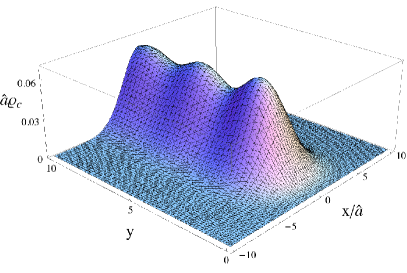
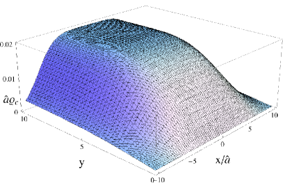
Figure 1: These 3d-plots show $\rho_{\rm c}$ for small lattice spacing ($\widehat{a}=0.1$, left figure) and for a large one ($\widehat{a}=1$, right figure). The index is $\nu=1$. Oscillations are well distinguishable for small $\widehat{a}$ whereas they disappear for larger lattice spacing. Notice that $\widehat{a}$ in the right figure is one order larger than in the left one.

In the microscopic limit ($n\to\infty$) we obtain [13]

$$\rho_{\rm c}\left(\frac{z}{2n}\right) = \frac{|y|}{(2\pi)^{5/2}2\widehat{a}}\int\exp(-\Delta_{1}^{2}-\Delta_{2}^{2}){\rm sinc}\left[\frac{y}{2\widehat{a}}(\Delta_{1}-\Delta_{2})\right]\cos\nu(\varphi_{1}+\varphi_{2})D\varphi_{k},$$ (14)

$$\rho_{\rm r}\left(\frac{x}{2n}\right) = \frac{1}{16\pi^{2}}\int\frac{\exp[\Delta_{1}^{2}-\Delta_{2}^{2}]{\rm erf}\left[\Delta_{1},\sqrt{2}\Delta_{1}\right]-\{\Delta_{1}\leftrightarrow\Delta_{2}\}}{\cos\varphi_{1}-\cos\varphi_{2}}\cos\nu(\varphi_{1}+\varphi_{2})D\varphi_{k},$$ (15)

$$\rho_{\chi}\left(\frac{x}{2n}\right) = \int\frac{(-\imath s_{1})^{\nu}}{16\pi\widehat{a}^{2}}\frac{e^{-((s_{1}-x)^{2}+(s_{2}+ix)^{2})/16\widehat{a}^{2}}}{s_{1}-\imath s_{2}}\det\left[\begin{array}[]{cc}s_{1}K_{\nu+1}(s_{1})&s_{2}J_{\nu+1}(s_{2})\\ K_{\nu}(s_{1})&J_{\nu}(s_{2})\end{array}\right]\frac{\delta^{(\nu-1)}(s_{1})}{(\nu-1)!}d[s].$$ (18)

The functions ${\rm sinc}$, ${\rm erf}$, $J_{l}$, $K_{l}$ and $\delta^{(l)}$ are the sinus cardinalis, the generalized incomplete error function (${\rm erf}(b,c)={\rm erf}(c)-{\rm erf}(b)$), Bessel function of the first kind, the modified one of the second kind and the $l$-th derivative of the $\delta$ function, respectively. We employed the abbreviations $D\varphi_{k}=\sin^{2}((\varphi_{1}-\varphi_{2})/2)d\varphi_{1}d\varphi_{2}$ and $\Delta_{j}=2\widehat{a}\left(\cos\varphi_{j}-{x}/{8\widehat{a}^{2}}\right)$. Notice that only the singular part of $K_{l}$ contributes due to the $\delta$ function and that $\rho_{\chi}$ vanishes for $\nu=0$.

For sufficiently small $\widehat{a}$, $\rho_{c}$ is broadened by a Gaussian along the imaginary axis, the oscillations of the continuum limit are distinct and near the real axis it behaves like $y^{\nu+1}$. When increasing the lattice spacing the oscillations disappear and the behavior near the real axis becomes independent of $\nu$ and $y$. The distribution $\rho_{\chi}$ develops a box-like shape along the imaginary axis with support $|x|\leq 8\widehat{a}^{2}$. In Fig. 1 we show 3D-plots of $\rho_{\rm c}$.

An important quantity to measure the effect of a finite lattice spacing is the average number of the additional real modes. It is given by [14]

$$N_{\rm add}=2\int_{\mathbb{R}}\rho_{\rm r}\left(\frac{x}{2n}\right)dx=\int_{0}^{2\pi}\frac{1-e^{-4\widehat{a}^{2}\sin^{2}\varphi}I_{0}(4\widehat{a}^{2}\sin^{2}\varphi)}{4\pi\sin^{2}\varphi}\cos 2\nu\varphi d\varphi\propto\left\{\begin{array}[]{cl}\widehat{a}^{2(\nu+1)},&\widehat{a}\ll 1,\\ \widehat{a},&\widehat{a}\gg 1.\end{array}\right.$$ (21)

At small lattice spacing contributions for non-zero index are suppressed whereas $N_{\rm add}$ for large $\widehat{a}$ is independent of the index. This is shown in Fig. 2.

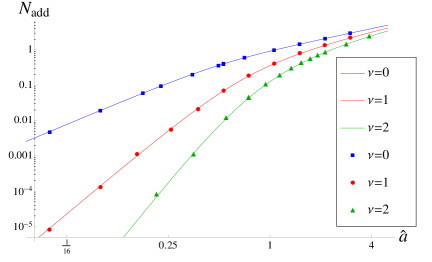
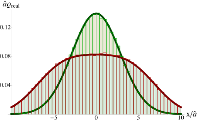
Figure 2: Left: Log-log-plot of the average number of additional real modes over $\widehat{a}$. The Monte Carlo simulations (symbols) confirm our analytical results (solid curves). The matrix dimension and the number of matrices vary in the simulations. Right: The distribution $\rho_{\rm real}$ is governed by $\rho_{\chi}$ at small $\widehat{a}$ (green, $\widehat{a}=1/\sqrt{200}$) but is increasingly dominated by $\rho_{\rm r}$ (red, $\widehat{a}=1/\sqrt{2}$). We compare our analytical results (solid curves) with Monte Carlo simulations (histograms, 200000 matrices, $n=50$, $\nu=1$, bin size is 0.4).

At small lattice spacing, the distribution of the real eigenvalues, $\rho_{\rm real}=\rho_{\rm r}+\rho_{\rm l}=2\rho_{\rm r}+\rho_{\chi}$, is approximated by the $\nu$-dimensional Gaussian unitary ensemble. The width is $2\widehat{a}$ in this regime. For increasing lattice spacing the support increases to $|x|\leq 8\widehat{a}^{2}$ (see Fig. 2) and develops a square root singularity at the edges, i.e. $\rho_{\rm real}(x)=1/[(2\pi)^{3/2}\widehat{a}]+\nu/[\pi\sqrt{(8\widehat{a}^{2})^{2}-x^{2}}]$. The first term is due to $\rho_{\rm r}$ while the singularity comes from $\rho_{\chi}$.

3 Staggered fermions

In this section we introduce an ensemble to study the taste breaking of the staggered Dirac operator. For simplicity we only consider the case of two tastes with the ensemble given by

$$D_{\rm st}=\left(\begin{array}[]{cccc}0&V\\ -V^{\dagger}&0\end{array}\right),\ V=\left(\begin{array}[]{cc}W+a_{1}\widetilde{W}&a_{2}C\\ a_{2}B&W^{\dagger}-a_{1}\widetilde{W}^{\dagger}\end{array}\right),\ P(D_{\rm st})\propto e^{-n(\textrm{tr}A^{2}/2+\textrm{tr}B^{2}/2+\textrm{tr}WW^{\dagger}+\textrm{tr}\widetilde{W}\widetilde{W}^{\dagger})},$$ (22)

where $W,\widetilde{W}$ are $n\times(n+\nu)$ and $B,C$ are $(n+\nu)\times(n+\nu)$ and $(n\times n)$ complex matrices respectively. The matrix dimension $n$ is identified with the spacetime volume $V$ as in the case of the Wilson Dirac operator. For $a=0$ this model has two flavors with $\nu$ zero modes for each flavor while at $a\neq 0$ with interacting tastes, the zero modes are absent and the continuum ${\rm SU}(2)$ flavor symmetry is broken. A more general random matrix model with four tastes and additional taste breaking terms was introduced in Ref. [15].

Studying the ensemble (22) in the limit, $n\to\infty$, at rescaled quark masses $\widehat{M}=2nM$ and lattice spacing $\widehat{a}_{j}^{2}=na_{j}^{2}/2$ allows us to obtain universal results for the eigenvalue correlations which will be worked out elsewhere. Here, we evaluate the partition function of $N_{\rm f}$ fermions corresponding to the matrix model (22) which is given by the unitary matrix integral

Z $$\propto \int_{{\rm U}(N_{\rm f})}dU{\det}^{\nu}U\exp\left[\widehat{a}_{1}^{2}\textrm{tr}[\tau_{3}U\tau_{3}U^{\dagger}]+\widehat{a}_{2}^{2}\textrm{tr}[(\tau_{1}U)^{2}+(\tau_{2}U)^{2}+\textrm{cc.}]-\textrm{tr}\widehat{M}(U+U^{\dagger})\right].$$ (23)

It agrees with the $\varepsilon$ limit of the staggered chiral Lagrangian corresponding to the taste breaking pattern of the ensemble (22), and is a special case of the result derived in Ref. [15].

The spectral flow as a function of $a$ shows avoided level crossings when lattice artifacts start dominating the Dirac spectrum (see Fig. 3 (left)). For small $a$ we observe a linear behavior that follows from perturbation theory. At $a=0$ all eigenvalues have a degeneracy of two. The matrix $\widetilde{W}$ in Eq. (22) lifts this degeneracy but does not give repulsion between the two subspectra. On the other hand, the matrices $B$ and $C$ lift the degeneracy and cause a repulsion between the subspectra.

For $\widehat{a}_{j}\ll 1$ the spectral density exhibits a chGUE with twice the number of flavors as for $\widehat{a}_{j}\gg 1$. At $a_{2}=0$ the distribution of the zero modes is given by a Dirac delta function with weight $2\nu$ at zero. For increasing $a_{2}$ the distribution of these modes broadens gradually. Because they repel each other as well as the other modes, we always find a vanishing eigenvalue density at zero.

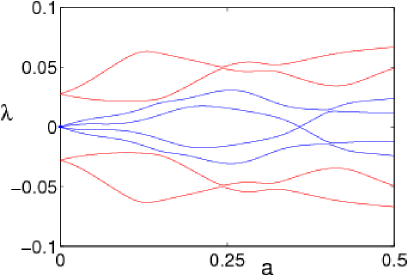
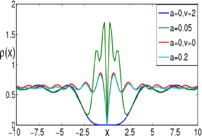
Figure 3: Left: The spectral flow of staggered eigenvalues for $\nu=2$ as a function of $a$ using a fixed realization of the random matrix ensemble (3.1) for $n=50$. The first avoided level crossing determines the perturbative regime. Right: The quenched spectral densities of $D_{\rm st}$ for values of $a$ (nonrescaled) and $\nu$ given in the legend of the figure obtained by Monte Carlo simulations with $n=50$ and $100000$ matrices. In both figures we set $a_{1}=a_{2}=a$.

4 Conclusions

For the Wilson-Dirac operator the discretization effects become strong when $\widehat{a}\gg 0.5$, i.e. $\widetilde{a}\gg 1/(2\sqrt{W_{8}V})$. Then characteristics of the continuum limit like the oscillations in the spectral density or its behavior near the real axis disappear. In the limit of large $\widehat{a}$, the eigenvalue distributions become independent of the index $\nu$, have a support in $|x|\leq 8W_{8}V\widetilde{a}^{2}$ and the distribution for the complex as well as for the eigenvalues of the right handed modes develop plateaus. The chirality distribution for large lattice spacing has square root singularities at the edges.

At sufficiently small lattice spacings the low energy constant $W_{8}$ can be extracted by combining the width of the Gaussian which broadens $\rho_{c}$ in the $x$ direction, $\sigma=2\widetilde{a}\sqrt{W_{8}/V}/\Sigma$, and the spacing of the projected eigenvalues onto the imaginary axis, $\Delta\lambda=\pi/\Sigma V$, yielding $\sigma/\Delta\lambda=2\widehat{a}/\pi$. Furthermore, additional real modes are highly suppressed by non-zero index $\nu$ and, thus, are not much of a problem in lattice QCD since most configurations have an index $|\nu|>0$ for large volumes.

The matrix model proposed above is the version with two tastes of the one in Ref. [15] and describes the main features of the low-lying spectrum of the two dimensional staggered Dirac operator. The scale $1/\sqrt{n}$ (i.e. $1/\sqrt{V}$ ) determines the appearance of lattice artifacts with increasing lattice spacing $a$. We expect that it is analytically solvable like the ensemble for the Wilson Dirac operator.

Acknowledgements.

We thank Kim Splittorff for simplifying Eq. (21) and other helpful comments. MK acknowledges financial support by the Alexander-von-Humboldt Foundation. JV and SZ acknowledge support by U.S. DOE Grant No. DE-FG-88ER40388.

References

- [1] E. V. Shuryak, J. J. M. Verbaarschot, Nucl. Phys. A 560, 306-320 (1993).
- [2] S. R. Sharpe, R. L. Singleton, Jr, Phys. Rev. D58, 074501 (1998); Nucl. Phys. Proc. Suppl. 73, 234-236 (1999); S. R. Sharpe, Phys. Rev. D 74, 014512 (2006).
- [3] G. Rupak and N. Shoresh, Phys. Rev. D 66, 054503 (2002).
- [4] S. Necco, A. Shindler, JHEP 1104, 031 (2011).
- [5] P. H. Damgaard, K. Splittorff and J. J. M. Verbaarschot, Phys. Rev. Lett. 105, 162002 (2010).
- [6] G. Akemann, P. H. Damgaard, K. Splittorff, J. J. M. Verbaarschot, PoS LATTICE2010, 079 (2010); PoS LATTICE2010, 092 (2010); Phys. Rev. D 83, 085014 (2011).
- [7] K. Splittorff, J. J. M. Verbaarschot, [hep-lat/1105.6229], (2011).
- [8] R. Kaiser, H. Leutwyler, Eur. Phys. J. C 17, 623-649 (2000).
- [9] G. Akemann, T. Nagao, [arXiv:1108.3035 [math-ph]] (2011).
- [10] L. Del Debbio, L. Giusti, M. Lüscher, R. Petronzio and N. Tantalo, JHEP 0602, 011 (2006); JHEP 0702, 056 (2007).
- [11] H.-J. Sommers and W. Wieczorek, J. Phys. A 41, 405003 (2008).
- [12] G. Akemann, E. Kanzieper, J. Stat. Phys. 129, 1158 (2007); G. Akemann, M. Kieburg, M. J. Phillips, J. Phys. A 43, 375207 (2010).
- [13] M. Kieburg, J. J. M. Verbaarschot and S. Zafeiropoulos, [arXiv:1109.0656 [hep-lat]] (2011).
- [14] We thank K. Splittorff for simplifying this result to a one-dimensional integral.
- [15] J. C. Osborn, Nucl. Phys. Suppl. 129, 886 (2004); Phys. Rev. D 83, 034505 (2011).
- [16] W.-J. Lee and S. R. Sharpe, Phys. Rev. D 60, 114503 (1999).