Hořava gravity vs. thermodynamics: the black hole case

Abstract

Under broad assumptions breaking of Lorentz invariance in gravitational theories leads to tension with unitarity because it allows for processes that apparently violate the second law of thermodynamics. The crucial ingredient of this argument is the existence of black hole solutions with the interior shielded from infinity by a causal horizon. We study how the paradox can be resolved in the healthy extension of Hořava gravity. To this aim we analyze classical solutions describing large black holes in this theory with the emphasis on their causal structure. The notion of causality is subtle in this theory due to the presence of instantaneous interactions. Despite this fact, we find that within exact spherical symmetry a black hole solution contains a space-time region causally disconnected from infinity by a surface of finite area – the ‘universal horizon’. We then consider small perturbations of arbitrary angular dependence in the black hole background. We argue that aspherical perturbations destabilize the universal horizon and, at non-linear level, turn it into a finite-area singularity. The causal structure of the region outside the singularity is trivial. If the higher-derivative terms in the equations of motion smear the singularity while preserving the trivial causal structure of the solutions, the thermodynamics paradox would be obviated. As a byproduct of our analysis we prove that the black holes do not have any non-standard long-range hair. We also comment on the relation with Einstein-aether theory, where the solutions with universal horizon appear to be stable.

1 Introduction and summary

There are several reasons for the current interest in gravitational models with broken Lorentz invariance (LI). First, these theories may be relevant in the quest for consistent alternatives to general relativity (GR) that modify the laws of gravity at large distances. (This search is in turn prompted by the attempts to resolve the problems of dark matter and dark energy raised by cosmological data.) Second, the construction of these models provides a necessary framework for testing the nature of LI. These motivations are behind the Einstein-aether model [1, 2], where Lorentz breaking is realized by a unit time-like vector field, and the ghost condensation model [3], where LI is broken by a scalar field with time-dependent vacuum expectation value (VEV). More complicated patterns of Lorentz breaking are realized in models of massive gravity [4], see [5] for a review.

More recently, this interest has been spurred by Hořava’s proposal [8] to construct a renormalizable model of quantum gravity by giving up LI. The main idea is that in the absence of LI the ultraviolet (UV) behavior of gravitational amplitudes can be substantially improved by the addition of terms with higher spatial derivatives to the action. This can be done while keeping the Lagrangian second order in time derivatives, thus avoiding problems with unstable degrees of freedom appearing in LI higher-derivative gravity [9]. The consistent implementation of this idea involves the notion of anisotropic (Lifshitz) scaling of the theory in the UV and indeed leads to a theory which is renormalizable by power-counting [8]. The renormalizability of the theory in the rigorous sense remains an open problem.

Lorentz violating gravitational models generically contain new degrees of freedom besides the two polarizations of the graviton. These degrees of freedom survive down to the infrared where they can be conveniently described as a new Lorentz violating sector interacting with Einstein’s general relativity. In this paper we will mainly focus on Hořava gravity. This model includes one new degree of freedom described by a scalar field $\varphi(x)$ with non-zero time-like gradient [10, 11],

$$\partial_{\mu}\varphi\neq 0~{},~{}~{}~{}~{}(\partial_{\mu}\varphi)^{2}>0\;.$$ (1)

Because of the latter property $\varphi$ can be chosen as a time coordinate and thus acquires the physical meaning of universal time; we will refer to it as ‘khronon’. The theory contains a mass scale $M_{*}$ assumed to be just a few orders of magnitude below the Planck mass and which suppresses the operators with higher derivatives. These operators are not important for the description of the khronon dynamics and its interaction with gravity at low energy. The low-energy properties are captured by an effective ’khronometric’ theory – a scalar-tensor theory satisfying certain symmetries [11]. It is worth mentioning that, as it is always the case for effective theories, the khronometric model is in a sense more general than Hořava gravity: given the symmetries and field content, it can be derived independently as the theory with the smallest number of derivatives in the action. In this paper we concentrate on the ‘healthy’ model proposed in [12, 13] which corresponds to the so called ‘non-projectable’ version of Hořava gravity. In this case the khronometric model possesses a symmetry under reparameterization of the khronon field,

$$\varphi\mapsto f(\varphi)\;,$$ (2)

where $f$ is an arbitrary monotonic function. Due to this symmetry the model differs essentially from ghost condensation, despite the fact that both are scalar-tensor theories with Lorentz violation. Instead, the model turns out to have a lot of similarities with the Einstein-aether theory [11, 14], without, however, being completely equivalent to it. Indeed, in addition to the scalar mode the aether contains two more propagating degrees of freedom corresponding to the transverse polarization of a vector field. On the other hand, the khronometric model includes instantaneous interactions [11] that are absent in the case of Einstein-aether. The phenomenological consequences of the khronometric model have been analyzed in [11, 15], where it was shown that for appropriate choice of parameters it satisfies the existing experimental constraints. In [16] it was shown that extending the model by an additional scalar field with exact shift symmetry allows to naturally account for the cosmological dark energy.

In this paper we study black hole (BH) solutions of the khronometric theory. These provide large distance (with respect to the scale $M_{*}^{-1}$) solutions of the healthy Hořava gravity, and are expected to be produced by gravitational collapse. One expects BHs in Hořava gravity to differ from those of GR in several aspects. In GR a BH is characterized by the existence of a horizon for light rays, which prevents the propagation of signals from its interior to the exterior. In this way, the horizon shields the central singularity of the BH from the exterior. However, in the presence of Lorentz violation the theory may contain excitations whose propagation velocity exceeds that of light and which thus can escape from inside GR horizons [17]. Moreover, in Hořava gravity the dispersion relations of the propagating degrees of freedom in the locally flat coordinate system have the form [8]

$$E^{2}=c^{2}_{n}p^{2}+\frac{a_{n}p^{4}}{M_{*}^{2}}+\frac{b_{n}p^{6}}{M_{*}^{4}}\;,$$ (3)

where $E$ and $p$ are the energy of the particle and its spatial momentum, and $c_{n}$, $a_{n}$, $b_{n}$ are coefficients of order one depending on the particle species $n$. Stability at high momenta requires the coefficient $b_{n}$ to be positive. This implies that both phase and group velocities of particles indefinitely grow with energy and one might think that these modes can come from the immediate vicinity of the central singularity. Finally, as we discuss in Sec. 2, even within the low-energy description in terms of the khronometric model the theory contains a certain type of instantaneous interactions, which again might probe the BH interior down to the center. This suggests that Hořava gravity does not allow for BHs in the strict sense, characterized by the existence of regions causally disconnected from the asymptotic infinity. The purpose of this article is to clarify if this expectation is true.

In our study we will be guided by the puzzles of BH thermodynamics arising in theories with Lorentz violation. As pointed out in [18, 19] for the examples of ghost condensation and Einstein-aether theories, one can construct gedanken experiments involving BHs that violate the second law of thermodynamics (see, however, [20] for a different point of view). Specifically, it is possible to set up processes that would decrease the entropy in the region outside the BH without any apparent change of the state of the BH itself. The second law of thermodynamics is intimately related to the unitarity of the underlying microscopic theory, see e.g. [21]. Thus its violation would constitute a serious problem, especially for a theory that, like Hořava gravity, aims at providing the microscopic description of quantum gravity. One can consider the following scenarios to recover the second law of thermodynamics:

• The missing entropy is accumulated somewhere inside the BH. The first guess for the precise location of the entropy storage region is close to the central singularity. In fact, this singularity is expected to be smeared off in the full theory at distances set by the microscopic scale and the entropy, in principle, can be stored in some high frequency modes localized in this smeared region. For this mechanism to work, an outside observer must be able to probe this region in order to make sure that the total entropy of the system does not decrease. This option seems plausible, given that Hořava gravity contains arbitrarily fast modes including an instantaneous mode that persists at low energies. However, one must check that these modes can indeed escape form the center of the BH. In other words, one has to work out the causal structure of BHs in this theory.

• Another possible scenario to restore the thermodynamics assumes that BHs are not uniquely characterized by their mass, but instead can come out in many different configurations [24]. In other words, it supposes that BHs have a large number of static long-range hair. This hair would grow during the processes suggested in [18, 19] and after measuring them an outer observer could decode the entropy fallen down into the BH. Notice that the difference with respect to the previous point is that the hair has a tail that can be measured outside the horizon. It has been demonstrated for several Lorentz violating theories including the Einstein-aether [22], ghost condensate [23] and massive gravity [24] that spherically symmetric solutions with given mass are unique. As we are going to see, this is also the case for the khronometric model. This implies that the hair necessarily must be non-spherical.

One of the purposes of this paper is to clarify which of these scenarios, if any, is realized in the healthy Hořava gravity. For this purpose, we first find spherical BH solutions in the khronometric model and analyze their causal structure. To simplify the analysis we will neglect the back-reaction of the khronon field on the metric. This approximation, valid when the dimensionless parameters of the khronon action are small, reduces the problem of finding the BH solution of the khronometric model to that of embedding the khronon field into a given metric background. We show in passing that these solutions also describe spherical BHs in the Einstein-aether theory. Next we consider perturbations on top of these solutions. We demonstrate that no static long-range hair exists thus rejecting option (ii). On the other hand, option (i) is likely to work, though in a quite non-trivial manner. Within spherical symmetry we find that, despite the presence of arbitrarily fast, viz. instantaneous, interactions, the center of the BH is shielded by a causal horizon. This ‘universal horizon’ lies inside the Schwarzschild radius and its size linearly depends on the BH mass. All fields of the spherically symmetric solution are regular (analytic) at this horizon. However, in the spectrum of non-spherical time-dependent perturbations one finds certain modes with non-analytic structure at the universal horizon. These modes precisely correspond to the instantaneous interactions of the khronometric theory. Though at the linear order the universal horizon turns out to be stable under perturbations, we argue that the above non-analyticities will destabilize it at non-linear level, turning it into a finite-area singularity. One hopes that in the full Hořava gravity this singularity is resolved into a high-curvature region of finite width accessible to the instantaneous and fast high-energy modes. In this way thermodynamics can be saved.

It is worth stressing that the presence of instantaneous interaction is crucial for the type of instability discussed in this paper. Consequently, the universal horizon is expected to be stable in the Einstein-aether theory where all modes propagate with finite velocities. At present we are unable to suggest any resolution of the paradox with BH thermodynamics in this theory.

Despite the vast literature on BHs in Hořava gravity, there has been only a few works dealing with the healthy extension in which we are interested. A class of spherically symmetric solutions of the healthy Hořava gravity was found in [25]. Those solutions differ, however, from the black holes considered in this paper. Ref. [26] has obtained spherically symmetric BHs in the Einstein-aether and khronometric theories by numerically solving the coupled system of equations for the metric and aether (khronon) field. Our approach is different in that we simplify the setup to use analytic techniques whenever possible. This allows us to go beyond the spherical symmetry and study aspherical perturbations around BHs. Where our results overlap with those of [26], they agree.

The paper is organized as follows. In Sec. 2 we introduce the khronometric model and demonstrate that it contains instantaneous interactions. In Sec. 3 we find spherical BHs and show that those are also solutions for Einstein-aether theory. We also analyze their causal structure in this section. We turn to the analysis of the khronon perturbations about the BH in Sec. 4. Section 5 is devoted to discussion. In Appendix A we show that the instantaneous interaction is absent in the Einstein-aether model. Appendix B contains certain analytic results about spherical BHs.

2 The khronometric model and instantaneous modes

The khronometric action corresponding to the low-energy limit of Hořava gravity has the form [11],

$$S=-\frac{M^{2}}{2}\int\mathrm{d}^{4}x\sqrt{-g}\bigg{[}R+\alpha(u^{\mu}\nabla_{\mu}u_{\nu})^{2}+\beta\nabla_{\mu}u^{\nu}\nabla_{\nu}u^{\mu}+\lambda(\nabla_{\mu}u^{\mu})^{2}\bigg{]}\;.$$ (4)

Here $R$ is the Ricci scalar and the unit vector $u_{\mu}$ is expressed in terms of the khronon field $\varphi$ as,

$$u_{\mu}\equiv\frac{\partial_{\mu}\varphi}{\sqrt{\partial_{\nu}\varphi\nabla^{\nu}\varphi}}\;.$$ (5)

In Eq. (4) $M$ is a mass parameter related to the Planck mass and $\alpha,\beta,\lambda$ are dimensionless constants. The previous action is the most general expression invariant under the transformations (2) and containing only two derivatives of $u_{\mu}$. Note that it formally coincides with the action of the Einstein-aether theory [1, 2]. The difference, however, is that in the case of Einstein-aether the unit vector $u_{\mu}$ is treated as a fully dynamical variable, subject only to the constraint of been a unit time-like vector, and thus contains additional transverse degrees of freedom compared to the khronometric model where it is written in terms of the scalar field $\varphi$. This difference disappears for spherically symmetric solutions, since the aether vector is always hypersurface-orthogonal in that case [22] and thus can be expressed in the form (5).

We assume that the parameters $\alpha,\beta,\lambda$ are small,

$$\alpha,~{}\beta,~{}\lambda\ll 1.$$ (6)

On one hand, this choice is motivated by the phenomenological bounds on the model [11, 15]. At the same time it drastically simplifies the rest of the analysis allowing to neglect the back-reaction of the khronon field on the metric. In fact, it is clear from (4) that the energy-momentum tensor of the khronon field is proportional to the parameters $\alpha,\beta,\lambda$ . Thus its contribution into the Einstein equations is negligible when these parameters satisfy (6). This implies that the problem of finding a solution of the theory is reduced to solving the khronon equation of motion in an external (background) metric.

A crucial property of the theory at hand is the presence of an instantaneous interaction [11]. To understand its origin one can consider the propagation of small khronon perturbations in Minkowski space-time. It is straightforward to see that the Ansatz $\varphi=t$ for the khronon background satisfies the equations of motion in this space-time. For the perturbations, we define a field $\chi$ on top of this background,

$$\varphi=t+\chi\;,$$ (7)

for which one obtains the following quadratic action:

$$S^{(2)}_{\varphi}=\frac{M^{2}}{2}\int\mathrm{d}^{4}x~{}\Big{[}\alpha(\partial_{i}\dot{\chi})^{2}-(\beta+\lambda)(\Delta\chi)^{2}\Big{]}\;.$$ (8)

Note that this action is fourth order in derivatives. However, the additional derivatives are purely space-like and the action describes a single wave mode with velocity

$$c_{\chi}=\sqrt{\frac{\beta+\lambda}{\alpha}}\;.$$ (9)

As shown in [11], this remains true also for curved backgrounds: the equation of motion for khronon perturbations always remain second order in time derivatives if the time coordinate is chosen to coincide with the background khronon field.

Still the presence of extra spatial derivatives implies instantaneous propagation of signals. To see this, let us couple the khronon field to a source. The simplest source term that preserves the symmetries of the khronon field has the form

$$S_{source}=\int\mathrm{d}^{4}x\sqrt{-g}\,S^{\mu}u_{\mu}\;,$$ (10)

where $S^{\mu}$ is the source vector. To linear order around the flat background this reads

$$S_{source}^{(1)}=\int\mathrm{d}^{4}x\;S^{i}\partial_{i}\chi\;,$$ (11)

which leads to the khronon exchange amplitude

$${\cal A}=M^{-2}S^{i}(x)G_{ij}(x-y)S^{j}(y)\;,$$ (12)

where

$$G_{ij}(x)=\int\frac{\mathrm{d}^{4}p}{(2\pi)^{4}}\frac{{\bf p}_{i}{\bf p}_{j}~{}{\rm e}^{-ipx}}{{\bf p}^{2}\big{(}\alpha p_{0}^{2}-(\beta+\lambda){\bf p^{2}}\big{)}}\;,$$ (13)

where $\theta$ is the step function and $\delta$ the Dirac delta-function. A straightforward calculation yields the retarded propagator:

$$G_{ij}^{ret}(x)=-\frac{\theta(t)\delta(|{\bf x}|-c_{\chi}t)}{4\pi\sqrt{\alpha(\beta+\lambda)}}\,\frac{{\bf x}_{i}{\bf x}_{j}}{|{\bf x}|^{3}}\,+\frac{\theta(t)\theta(|{\bf x}|-c_{\chi}t)}{4\pi\alpha}\,\left(\frac{3{\bf x}_{i}{\bf x}_{j}-\delta_{ij}|{\bf x}|^{2}}{|{\bf x}|^{5}}\right)t\;.$$ (14)

Clearly, due to the second term the retarded Green’s function does not vanish outside the khronon ‘sound cone’ $c_{\chi}t=|{\bf x}|$. Moreover, the field extends to arbitrary spatial distance from the source immediately after the source is switched on, meaning that the signal propagates instantaneously. Note, however, that the instantaneous part of the signal builds up gradually starting from zero at $t=0$ and the maximum amplitude that is reached by the time $t=|{\bf x}|/c_{\chi}$ decreases with the distance as $1/|{\bf x}|^{2}$. This is similar to the situation in Lorentz violating massive electrodynamics [28, 29] and massive gravity [24, 30]. It is worth stressing that due to the existence of a preferred frame the instantaneous propagation of signals does not lead to any inconsistencies.

Note that the instantaneous piece in (14) is traceless and transverse,

$$G_{ii}^{ret,\,inst}(x)=\partial_{i}G_{ij}^{ret,\,inst}(x)=0\;.$$

The latter property implies that the instantaneous contribution will vanish if the source $S^{\mu}(x)$ is a gradient of a localized scalar configuration. We also point out that, despite the similarity between the khronometric and Einstein-aether theories, the latter does not contain any instantaneous interactions. As shown in the Appendix A, the instantaneous piece in (14) is canceled by the contributions of the transverse modes.

3 Spherical black holes

3.1 Preliminaries

According to the discussion of the previous section, our method to find BH solutions will consist in embedding the khronon field in an external BH metric. The latter satisfies the gravitational equations of motion in the vacuum. In the spherically symmetric case we will start with the standard Schwarzschild metric in the Schwarzschild coordinates,

$$\mathrm{d}s^{2}=\left(1-\frac{r_{s}}{r}\right)\mathrm{d}t^{2}-\frac{\mathrm{d}r^{2}}{1-\frac{r_{s}}{r}}-r^{2}\mathrm{d}\Omega^{2}\;,$$ (15)

where

$$\mathrm{d}\Omega^{2}=\mathrm{d}\theta^{2}+\sin^{2}\theta\mathrm{d}\phi^{2}\;,$$ (16)

is the area element of the 2-sphere and $r_{s}$ is the Schwarzschild radius. Using the Finkelstein coordinate

$$v=t+r+r_{s}\mathop{\rm ln}\nolimits{\bigg{(}\frac{r}{r_{s}}-1\bigg{)}}\;,$$ (17)

the previous metric can be cast into the form regular at the Schwarzschild horizon,

$$\mathrm{d}s^{2}=\left(1-\frac{r_{s}}{r}\right)\mathrm{d}v^{2}-2\mathrm{d}v\mathrm{d}r-r^{2}\mathrm{d}\Omega^{2}\;.$$ (18)

To simplify the khronon action, one observes that the curl of a hypersurface-orthogonal vector (5) identically vanishes,

$$\omega_{\mu}\equiv\epsilon_{\mu\nu\lambda\rho}u^{\nu}\nabla^{\lambda}u^{\rho}=0\;.$$ (19)

This implies

$$0=\omega_{\mu}\omega^{\mu}=-\frac{1}{2}u_{\mu\nu}u^{\mu\nu}+(u^{\nu}\nabla_{\nu}u_{\mu})^{2}\;,$$ (20)

where

$$u_{\mu\nu}\equiv\partial_{\mu}u_{\nu}-\partial_{\nu}u_{\mu}\;.$$ (21)

Furthermore,

$$\beta\int\mathrm{d}^{4}x\sqrt{-g}\nabla_{\mu}u_{\nu}\nabla^{\nu}u^{\mu}=\beta\int\mathrm{d}^{4}x\sqrt{-g}\big{[}(\nabla_{\mu}u^{\mu})^{2}-R_{\mu\nu}u^{\mu}u^{\nu}\big{]}$$ (22)

where $R_{\mu\nu}$ is the background Ricci tensor. Combining (20) and (22) we obtain that in the Schwarzschild geometry the khronon action can be written in the equivalent form

$$S_{\varphi}=-M^{2}\int\mathrm{d}^{4}x\sqrt{-g}\bigg{(}\frac{\alpha}{4}u_{\mu\nu}u^{\mu\nu}+\frac{\beta+\lambda}{2}(\nabla_{\mu}u^{\mu})^{2}\bigg{)}\;,$$ (23)

where we have used that the Ricci tensor for the Schwarzschild metric vanishes.

The khronon equation of motion, following from the variation of (23) with respect to $\varphi$, has the form of a current conservation,

$$\nabla_{\mu}J^{\mu}=0\;,$$ (24)

with

$$J^{\mu}=\frac{P^{\mu}_{\nu}}{\sqrt{X}}\,\frac{\delta S_{\varphi}}{\delta u_{\nu}}\;.$$ (25)

Here $X=\partial_{\mu}\varphi\nabla^{\mu}\varphi$ and

$$P^{\mu}_{\nu}=\delta^{\mu}_{\nu}-u^{\mu}u_{\nu}\;$$ (26)

is the projector on the hypersurface orthogonal to $u^{\mu}$; this implies

$$u_{\mu}J^{\mu}=0\;$$ (27)

We are interested in static, spherically symmetric, asymptotically flat solutions of (24). In the present context these notions require some clarification. The condition of staticity does not mean that the khronon field is independent of time (indeed, we saw that in the case of the Minkowski background $\varphi$ grows linearly with time). Rather it implies that all quantities invariant under the symmetry (2) must be constant in time. In particular, this applies to the components of the vector $u_{\mu}$. Combined with the requirement of spherical symmetry, this implies that the only non-vanishing components of the vector are $u_{t}$, $u^{r}$ and that they depend only on the radial coordinate $r$. Note that we have chosen the position of the index ’$t$’ – down and ’$r$’ – up so that the corresponding components of the vector coincide in the Schwarzschild and Finkelstein frames:

$$u_{v}=u_{t}~{},~{}~{}~{}u^{r}\big{|}_{Finkelstein}=u^{r}\big{|}_{Schwarzschild}\;.$$

For the khronon field itself, staticity and spherical symmetry imply that, up to a reparameterization of the form (2), it can be cast into the form

$$\varphi=t+f(r)\;,$$ (28)

where $f(r)$ is a function of the radius. Concerning the condition of the asymptotic flatness, we will impose, in addition to the flatness of the metric at $r\to\infty$, the requirement that the khronon field tends to the same form as in Minkowski space-time, $\varphi=t$. This implies the boundary conditions at infinity:

$$u_{t}\to 1~{},~{}~{}~{}u^{r}\to 0~{},~{}~{}~{}\sqrt{X}\to 1~{}~{}~{}~{}~{}~{}~{}\text{at}~{}~{}r\to\infty\;.$$ (29)

We now prove that asymptotically flat static spherically symmetric solutions of (24) satisfy the stronger equation

$$J^{\mu}=0\;.$$ (30)

Taking the first integral of Eq. (24) we obtain

$$J^{r}=\frac{C_{1}}{r^{2}}\;,$$ (31)

where $C_{1}$ is an integration constant. On the other hand, the explicit expression for $J^{r}$ in terms of $u_{\mu}$ reads,

$$J^{r}=\frac{1}{\sqrt{X}}\bigg{[}\alpha\,u^{r}u_{t}\bigg{(}\partial_{r}^{2}u_{t}+\frac{2}{r}\partial_{r}u_{t}\bigg{)}-(\beta+\lambda)u_{t}^{2}\partial_{r}\bigg{(}\partial_{r}{u^{r}}+\frac{2}{r}u^{r}\bigg{)}\bigg{]}\;,$$ (32)

where the components of the vector satisfy the unit norm constraint

$$u_{t}^{2}-(u^{r})^{2}=1-\frac{r_{s}}{r}\;.$$ (33)

After substituting (31) into (32) and expanding the r.h.s. of (32) at large $r$, the solution of the resulting linear differential equation reads

$$u^{r}=\frac{C_{1}}{2(\beta+\lambda)}+\frac{C_{2}}{r^{2}}+C_{3}r\;,$$ (34)

where $C_{2}$, $C_{3}$ are integration constants. We see that the only solution compatible with the boundary conditions (29) is obtained for the choice $C_{1}=C_{3}=0$. This implies $J^{r}=0$. Finally, from (27) one finds that $J^{t}$ is also zero.

We point out that Eq. (30) is the same as the equation of motion for the Einstein-aether model. Indeed, the latter is obtained by the variation of the action (23) with respect to the vector $u_{\mu}$ imposing that the variations of the vector components preserve the constraint $u_{\mu}u^{\mu}=1$. This leads to the appearance of the projector $P^{\mu}_{\nu}$ in the expression (25) for $J^{\mu}$. Together with the fact that spherically symmetric solutions are always hypersurface-orthogonal [14] this proves that static spherically symmetric asymptotically flat solutions in the khronometric and Einstein-aether theories are equivalent.

3.2 Solutions

Our strategy to find the khronon configuration corresponding to a BH will be as follows. We solve the equation $J^{r}=0$ for the vector $u_{\mu}$, and afterwards reconstruct the corresponding khronon field. Introducing the notations

$$U\equiv u_{t}~{},~{}~{}~{}V\equiv u^{r}~{},~{}~{}~{}\xi\equiv\frac{r_{s}}{r},$$ (35)

equations (30) and (33) take the form,

$$\frac{U^{\prime\prime}}{U}-c_{\chi}^{2}\frac{V^{\prime\prime}}{V}+\frac{2c^{2}_{\chi}}{\xi^{2}}=0\;,$$ (36a)

$$U^{2}-V^{2}=1-\xi\;,$$ (36b)

where prime denotes differentiation with respect to $\xi$. Note that in the new coordinate the position of the Schwarzschild horizon is $\xi=1$, the region $\xi<1$ lies outside this horizon, while $\xi>1$ corresponds to the black hole interior. Expressing $V$ from (36b)

$$V=-\sqrt{U^{2}-1+\xi}$$ (37)

we obtain a single equation for the $U$ component:

$$U^{\prime\prime}+\frac{c^{2}_{\chi}U}{U^{2}(1-c^{2}_{\chi})-1+\xi}\bigg{[}-(U^{\prime})^{2}+\frac{(UU^{\prime}+1/2)^{2}}{U^{2}-1+\xi}+\frac{2(U^{2}-1+\xi)}{\xi^{2}}\bigg{]}=0\;.$$ (38)

One observes that the denominator in the second term vanishes at the point $\xi_{c}$ where

$$(1-c_{\chi}^{2})U^{2}(\xi_{c})=1-\xi_{c}\;.$$ (39)

This is nothing but the equation determining the position of the sound horizon for the propagating khronon mode. Indeed, we saw in Sec. 2 that in Minkowski space-time with the vector $u_{\mu}$ aligned along the time direction the wave component of the khronon propagates along the rays $|{\bf x}|=c_{\chi}t$. Denoting the tangent vectors to these rays by $n_{\mu}$ we find that they satisfy

$$n_{\mu}n^{\mu}=(1-c^{2}_{\chi})(u_{\mu}n^{\mu})^{2}\;.$$ (40)

This equation has covariant form and straightforwardly generalizes to curved backgrounds with generic vector $u_{\mu}$ where it describes the sound cone for the khronon waves. The defining property of the sound horizon is that inside it all future-directed khronon rays point towards the center, $n^{r}<0$ for any $n^{\mu}$ satisfying (40) and $n^{v}>0$, while outside of it the sign of $n^{r}$ can be positive. This implies that at the sound horizon the sound cone contains the vector $n^{\mu}=(1,0,0,0)$. Substituting this into (40) and using the metric (18) we obtain (39). Clearly, for the subluminal khronon, $c_{\chi}<1$, the sound horizon lies outside the Schwarzschild horizon, $\xi_{c}<1$, while for the superluminal case $c_{\chi}>1$, the situation is opposite, $\xi_{c}>1$; for $c_{\chi}=1$ both horizons coincide.

We are interested in khronon embeddings with a regular future sound horizon that are expected to appear as the result of a gravitational collapse. The regularity of the solution at the sound horizon implies that the term within the square brackets in (38) must vanish at $\xi_{c}$. This imposes a relation between the first derivative $U^{\prime}$ and the function $U$ itself at this point, providing an additional boundary condition. Using (39) to simplify the formulas we obtain,

$$U^{\prime}(\xi_{c})=\frac{1}{2(1-c_{\chi}^{2})U(\xi_{c})}\bigg{[}-1+c_{\chi}\sqrt{1-\frac{8c_{\chi}^{2}(1-c_{\chi}^{2})U^{4}(\xi_{c})}{\xi_{c}^{2}}}\bigg{]}\;,$$ (41)

where we have chosen the branch of the square root that gives a regular result at $c_{\chi}=1$.

We solved Eq. (38) numerically imposing the boundary conditions (39), (41) and

$$U(\xi=0)=1.$$ (42)

This was done using a shooting procedure where the shooting parameter is taken to be the value of the field at the sound horizon, $U(\xi_{c})$. This determines the positions $\xi_{c}$ of the sound horizon and the first derivative of the field there through (39), (41). Given $U(\xi_{c})$ and $U^{\prime}(\xi_{c})$ we integrate Eq. (38) from $\xi_{c}$ towards $\xi=0$ to find $U(0)$. Iterating this procedure we find the value $U(\xi_{c})$ that allows to satisfy (42). Finally, we extend the solution inside the sound horizon by solving Eq. (38) from $\xi_{c}$ to $\xi\to\infty$. In this way we obtain a unique solution for every value of $c_{\chi}$.

Figure 1: The time component $U\equiv u_{t}$ of the vector $u_{\mu}$ on the BH solution for several values of the khronon sound speed; the coordinate $\xi$ is related to the radius as $\xi\equiv r_{s}/r$.

The resulting profiles $U(\xi)$ are plotted in Fig. 1 for several values of the khronon sound speed $c_{\chi}$. A few characteristics of the solutions are listed in Table 1. An important property, that is immediately clear from Fig. 1, is the existence of roots of the function $U(\xi)$ (i.e. points where $U(\xi)$ crosses zero). In Appendix B the existence of at least one root is proven analytically for any value of $c_{\chi}$. Moreover, the numerical analysis indicates that the number of roots is actually infinite with the function $U(\xi)$ exhibiting an oscillatory behavior around the zero axis. (The beginning of the oscillations is clearly visible in Fig. 1 for the curve corresponding to $c_{\chi}=10$; for smaller values of $c_{\chi}$ the oscillations lie outside the range shown in the figure.) This is in agreement with the findings of [26].

Let us denote the smallest root of $U(\xi)$ by $\xi_{\star}$. Its values for the numerical solutions at different $c_{\chi}$ are listed in Table. 1. One observes that it mildly depends on the sound speed and satisfies $\xi_{\star}>1$, $\xi_{\star}>\xi_{c}$. One can show that $\xi_{\star}$ varies from $2$ for $c_{\chi}\to 0$ to $4/3$ when $c_{\chi}\to\infty$, see Appendix B. In the three-dimensional space the point $\xi_{\star}$ corresponds to a two-sphere lying inside the Schwarzschild and sound horizons. We are going to see that this sphere plays a special role in the causal structure of the khronometric BHs.

The last quantity presented in Table 1 is the derivative of the function $U$ at $\xi_{\star}$, $U^{\prime}_{\star}\equiv U^{\prime}(\xi_{\star}).$ These numerical data will be used below.

$c_{\chi}$	$\xi_{c}$	$\xi_{\star}$	$U^{\prime}_{\star}$
0.2	0.52	1.63	-0.647
0.5	0.81	1.48	-0.764
0.75	0.93	1.44	-0.819
1	1	1.41	-0.858
1.5	1.09	1.38	-0.906
2	1.14	1.37	-0.934
10	1.28	1.337	-1.032
100	1.328	1.333	-1.058

Table 1: Several characteristics of the black hole solutions for different values of $c_{\chi}$. See the text for definitions.

3.3 The universal horizon

Let us now study the khronon configuration corresponding to the BH solution. Taking the Ansatz

$$\varphi=v+\varphi_{1}(\xi)\;$$ (43)

and recalling the definitions (5), (35) we obtain the equation

$$\varphi^{\prime}_{1}=\frac{u_{\xi}}{u_{v}}=\frac{-V(\xi)-U(\xi)}{\xi^{2}(\xi-1)U(\xi)}\;,$$ (44)

where, to avoid proliferation of multiplicative factors $r_{s}$, we have set $r_{s}=1$; this convention will be adopted from now on. It is straightforward to obtain the solution in the vicinity of $\xi=\xi_{\star}$. Expanding the r.h.s. of (44) we obtain ,

$$\varphi_{1}(\xi)\approx\frac{1}{\xi_{\star}^{2}U^{\prime}_{\star}\sqrt{\xi_{\star}-1}}\log{(\xi_{\star}-\xi)}~{}~{}~{}~{}~{}\mathrm{at}~{}\xi\approx\xi_{\star}\;.$$ (45)

We observe that the khronon field logarithmically diverges at $\xi_{\star}$. This implies that the leaves of constant khronon coming from the spatial infinity accumulate at $\xi_{\star}$. None of them penetrate inside the region $\xi>\xi_{\star}$. In other words, the leaves foliating the interior of the sphere $\xi=\xi_{\star}$ are disconnected from the spatial infinity. This fact is illustrated in Fig. 2 where the khronon foliation is superimposed on the part of the BH Penrose diagram covered by the Finkelstein coordinates.

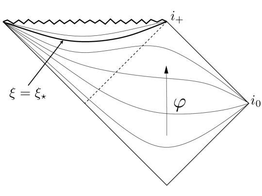
Figure 2: The leaves of constant khronon field (thin solid lines) superimposed on the upper half of the Penrose diagram of the Schwarzschild black hole. The thick solid line shows the universal horizon.

The situation is similar to what happens in GR for solutions containing Cauchy horizons. In both cases, the maximally extended solution contains more than one connected (asymptotic) region where boundary conditions should be specified. In the khronometric case, to know the solution at $\xi\geq\xi_{\star}$, one needs to specify the boundary conditions for the instantaneous mode not only at $i_{0}$, but also at $i_{+}$ (see Fig. 2).

On the other hand, the sphere $\xi=\xi_{\star}$ simultaneously plays the role of the universal causal horizon. Indeed, the khronon field sets the global time in the model at hand. All signals, no matter how fast, can propagate only forward in this global time. In this way the configuration of the khronon determines the causal structure of space-time in Hořava gravity. From Fig. 2 it is clear that within this causal structure the inner region $\xi>\xi_{\star}$ lies in the future with respect to the outer part of the space-time. Thus no signal can escape from inside the surface $\xi=\xi_{\star}$ to infinity (null asymptotic region between $i_{+}$ and $i_{0}$) meaning that this surface is indeed a universal horizon, cf. [26].

It should be pointed out that within the spherically symmetric approximation that we have adopted so far the universal horizon is regular, despite the apparent singularity (45) of the khronon. Indeed, we have seen above that the field $u_{\mu}$, which is the proper invariant observable of the theory, is smooth at $\xi=\xi_{\star}$. This implies that the singularity (45) can be removed by the symmetry transformation of the form (2). It is easy to see that the transformation

$$\varphi\mapsto\tilde{\varphi}=\exp\big{[}(\xi_{\star}^{2}U^{\prime}_{\star}\sqrt{\xi_{\star}-1})\;\varphi\big{]}\;$$

does the job: the redefined khronon field is analytic at $\xi_{\star}$. However, in the next section we will argue that the universal horizon exhibits non-linear instability against aspherical perturbations of the khronon field, which turn it into a physical singularity.

4 Beyond spherical symmetry: perturbations

4.1 Generalities

The existence of the universal horizon seems to exclude the option (i) for the resolution of the thermodynamical paradoxes mentioned in the Introduction. However, this conclusion is premature: one has to analyze the stability of the causal structure depicted in Fig. 2 before making a definite statement. To this end we now study linear perturbations of the khronon on top of the BH solutions found in the last section. This will also allow us to explore the option (ii), namely possible existence of hair. As the background solution is not known in analytic form, we will characterize it by functions $U(\xi)$, $V(\xi)$ as defined in (35) and obeying Eqs. (36).

The analysis of the khronon perturbations must be performed in the preferred frame related to the background khronon foliation. In this frame the equations for the perturbations are second order in time, despite the presence of higher spatial derivatives [10, 11, 14]. Thus we introduce a new time coordinate $\tau$ that coincides with the background khronon,

$$\tau=v+\varphi_{1}(\xi)\;,$$ (46)

where $\varphi_{1}$ obeys Eq. (44). In the new coordinates the metric takes the form,

$$\mathrm{d}s^{2}=(1-\xi)\mathrm{d}\tau^{2}-\frac{2V}{\xi^{2}U}\mathrm{d}\tau\mathrm{d}\xi-\frac{\mathrm{d}\xi^{2}}{\xi^{4}U^{2}}-\frac{\mathrm{d}\Omega^{2}}{\xi^{2}}\;.$$ (47)

Note that this metric is singular at $\xi=\xi_{\star}$ and thus only covers the region outside the universal horizon. This is sufficient for our purposes as we restrict to perturbations localized in this region. The complete khronon field is written as

$$\varphi=\tau+\chi(\tau,\xi,\theta,\phi)\;,$$ (48)

where $\chi$ is a small perturbation. Due to the spherical symmetry of the problem, different spherical harmonics of $\chi$ decouple from each other at the linear level, which allows to consider the equations separately for each multipole component $\chi_{l}$. The latter obeys the relation

$$\Delta_{S^{2}}\chi_{l}=-L^{2}\chi_{l}\;,$$ (49)

where $\Delta_{S^{2}}$ is the Laplacian on the unit 2-sphere and $L^{2}\equiv l(l+1)$. To simplify notations we will omit the multipole label $l$ on $\chi$ in what follows.

Instead of directly linearizing the equations of motion, we find it convenient to consider the quadratic action for the perturbations. Substituting (47), (48) into (23) after a straightforward (though somewhat lengthy) calculation one obtains,

$$\begin{split}S^{(2)}_{\varphi}=2\pi M^{2}\alpha\int\mathrm{d}\tau\mathrm{d}\xi\bigg{[}U^{2}(\dot{\chi}^{\prime})^{2}&+\frac{L^{2}}{\xi^{2}}\dot{\chi}^{2}-2\xi^{2}U^{3}V\dot{\chi}^{\prime}\chi^{\prime\prime}-2L^{2}UV\dot{\chi}\chi^{\prime}\\ &+A(\xi)(\chi^{\prime\prime})^{2}+B_{l}(\xi)(\chi^{\prime})^{2}+C_{l}(\xi)\chi^{2}\bigg{]}\;.\end{split}$$ (50)

The coefficient functions $A$, $B_{l}$, $C_{l}$ are expressed in terms of $U$, $V$ and their derivatives:

$$A(\xi)= \xi^{4}U^{4}(V^{2}-c_{\chi}^{2}U^{2})\;,$$ (51a)

$$B_{l}(\xi)= -2\xi^{4}U^{3}V^{2}U^{\prime\prime}-\xi^{4}U^{4}VV^{\prime\prime}-2\xi^{4}U^{2}V^{2}{U^{\prime}}^{2}-2\xi^{2}U^{4}V^{2}-4\xi^{4}U^{3}U^{\prime}VV^{\prime}$$ (51b)

$$-4\xi^{3}U^{4}VV^{\prime}-8\xi^{3}U^{3}U^{\prime}V^{2}+L^{2}\xi^{2}U^{2}V^{2}-\xi^{4}U^{5}U^{\prime\prime}-2\xi^{4}U^{3}V^{2}U^{\prime\prime}$$

$$-c_{\chi}^{2}\big{(}-6\xi^{4}U^{4}{U^{\prime}}^{2}-12\xi^{3}U^{5}U^{\prime}-3\xi^{4}U^{5}U^{\prime\prime}+2L^{2}\xi^{2}U^{4}+6\xi^{2}U^{4}V^{2}-3\xi^{4}U^{4}VV^{\prime\prime}\big{)}\;,$$

$$C_{l}(\xi)= -L^{2}\big{[}2\xi\,UU^{\prime}V^{2}+\xi^{2}UV^{2}U^{\prime\prime}+2\xi^{2}UVU^{\prime}V^{\prime}+\xi^{2}U^{2}{U^{\prime}}^{2}+\xi^{2}U^{3}U^{\prime\prime}$$ (51c)

$$-c_{\chi}^{2}\big{(}-L^{2}U^{2}+\xi^{2}U^{3}U^{\prime\prime}+3\xi^{2}U^{2}{U^{\prime}}^{2}+10\xi U^{3}U^{\prime}+2U^{4}-2U^{2}V^{2}+\xi^{2}U^{2}VV^{\prime\prime}\big{)}\big{]}\;.$$

Note that the coefficient $A$ does not depend on the multipole number $l$. In deriving (50) and (51) we made use of the background equations of motion and integrated by parts to minimize the number of different $\chi$-structures appearing in the action. Note that the action (50) contains only two time-derivatives, as expected.

Before analyzing the equation of motion following from (50) let us discuss the boundary conditions that must be imposed on the solutions. First, the field $\chi$ must vanish at the spatial infinity, i.e. at $\xi\to 0$. Second, $\chi$ must be regular at the sound horizon $\xi=\xi_{c}$. Note that the latter corresponds to a zero of the coefficient $A(\xi)$. Determining the correct boundary conditions at the universal horizon is slightly more complicated due to the singularity of the metric (47) at $\xi_{\star}$. To bypass this obstacle consider the linear perturbations of the vector $u_{\mu}$:

$$u^{(1)}_{\tau}=\xi^{2}U^{2}V\chi^{\prime}~{},~{}~{}~{}u^{(1)\,\xi}=-\xi^{4}U^{3}\chi^{\prime}~{},~{}~{}~{}u^{(1)}_{\theta}=U\partial_{\theta}\chi~{},~{}~{}~{}u^{(1)}_{\phi}=U\partial_{\phi}\chi\;.$$ (52)

Here the positions of the upper and lower indices are chosen in such a way that the presented components are invariant under the coordinate change (46). Thus they also define the vector $u_{\mu}$ in the Finkelstein frame. We will require that the perturbations $u_{\mu}^{(1)}$ in the latter frame are bounded at the universal horizon. This is compatible with the assumption that the black hole represents the end point of the gravitational collapse of a smooth initial configuration. From (52) we see that this requirement is equivalent to the condition that $\chi$ diverges at $\xi_{\star}$ not faster than $|\xi-\xi_{\star}|^{-1}$. We will see that imposing this condition is enough for our purposes.

As a final remark we note that the expressions (51) considerably simplify in the case $c_{\chi}=1$,

$$A= \xi^{4}(\xi-1)U^{4}\;,$$ (53a)

$$B_{l}= 2\xi^{4}(1-\xi)(U^{2}+V^{2}){V^{\prime}}^{2}-2\xi^{4}(1-\xi)VV^{\prime}+8\xi^{3}(1-\xi)U^{2}VV^{\prime}$$

$$-\frac{\xi^{4}}{2}V^{2}+\xi^{4}U^{2}-4\xi^{3}(1-\xi)U^{2}-2\xi^{3}U^{4}+L^{2}\xi^{2}U^{2}V^{2}-2L^{2}\xi^{2}U^{4}\;,$$ (53b)

$$C_{l}= -L^{2}\big{[}(2\xi V^{2}-10\xi U^{2}+\xi^{2})UU^{\prime}-2U^{4}+L^{2}U^{2}\big{]}\;,$$ (53c)

where we have used the background equations (36) to simplify the final expressions.

4.2 Static perturbations: absence of hair

Now we can prove that the khronometric BHs do not possess long range hair. At linear level such hair would manifest itself in the form of regular static perturbations of the khronon field (cf. [24]). These obey the equation

$$(A(\xi)\chi^{\prime\prime})^{\prime\prime}-(B_{l}(\xi)\chi^{\prime})^{\prime}+C_{l}(\xi)\chi=0\;.$$ (54)

Let us count the number of free parameters of the general solution of Eq. (54) and compare it with the number of boundary conditions. Consider the asymptotics of the equation at spatial infinity, $\xi\to 0$. Keeping the leading terms in the functions $A,B_{l},C_{l}$, cf. (51), we obtain,

$$-(\xi^{4}\chi^{\prime\prime})^{\prime\prime}+2L^{2}(\xi^{2}\chi^{\prime})^{\prime}+L^{2}(2-L^{2})\chi=0\;.$$ (55)

We will look for solutions of the power-law form, $\chi\propto\xi^{\delta}$. Substituting this Ansatz into (55) and solving the resulting algebraic equation for $\delta$ one finds four roots:

$$\delta_{1}=l-1~{},~{}~{}~{}\delta_{2}=-l~{},~{}~{}~{}\delta_{3}=l+1~{},~{}~{}~{}\delta_{4}=-l-2\;.$$ (56)

Note that for $l=0$ we recover the asymptotics (34). For $l\geq 1$ the solutions corresponding to $\delta_{2,4}$ grow at infinity and must be rejected. Thus we are left with a two-parameter family of decaying solutions,

$$\chi\sim\chi_{1}\xi^{l-1}+\chi_{3}\xi^{l+1}\;.$$ (57)

These are further constrained by the boundary conditions at the universal and sound horizons. Expanding Eq. (54) at $\xi_{\star}$ we obtain

$$(\xi_{\star}^{4}(\xi_{\star}-1){U^{\prime}_{\star}}^{4}(\xi-\xi_{\star})^{4}\chi^{\prime\prime})^{\prime\prime}+\Big{(}(\xi_{\star}-1)\xi_{\star}^{2}{U_{\star}^{\prime}}^{2}(2\xi_{\star}^{2}{U_{\star}^{\prime}}^{2}-L^{2})(\xi-\xi_{\star})^{2}\chi^{\prime}\Big{)}^{\prime}=0\;.$$ (58)

Substituting the power-law Ansatz

$$\chi\propto(\xi-\xi_{\star})^{\gamma}$$ (59)

we obtain for the exponent

$$\gamma_{1}=0~{},~{}~{}~{}\gamma_{2}=-1~{},~{}~{}~{}\gamma_{\pm}=-\frac{1}{2}\pm\sqrt{\frac{1}{4}+\frac{L^{2}}{\xi_{\star}^{2}{U^{\prime}_{\star}}^{2}}}\;.$$ (60)

Recalling that $\chi$ must grow not faster than $|\xi-\xi_{\star}|^{-1}$ we obtain that the solution corresponding to $\gamma_{-}$ is excluded. This gives one equation on the two parameters $\chi_{1}$, $\chi_{3}$. One more equation follows from the requirement of regularity at the sound horizon $\xi=\xi_{c}$. Thus in total we have two equations for two parameters. Assuming that this system is not degenerate we conclude that the unique solution is $\chi_{1}=\chi_{3}=0$ implying the absence of hair.

The fact that the equations following from the boundary conditions are indeed non-degenerate can be explicitly verified in the case of high multipoles, $L^{2}\gg 1$. For the sake of the argument, we restrict to the case $c_{\chi}=1$, where the coefficients $A,B_{l},C_{l}$ simplify, see Eqs. (53). Keeping only the leading terms in $L^{2}$ in Eq. (54) we obtain,

$$(\xi^{4}U^{4}(\xi-1)\chi^{\prime\prime})^{\prime\prime}+L^{2}\Big{(}(-\xi^{2}U^{2}V^{2}+2\xi^{2}U^{4})\chi^{\prime}\Big{)}^{\prime}-L^{4}U^{2}\chi=0\;.$$ (61)

The form of this equation suggests to use the WKB method. Thus we search for the solutions using the expansion,

$$\chi(\xi)=\exp[L\,\sigma(\xi)+\ldots]\;.$$ (62)

Substituting this into (61) and restricting to the leading order $O(L^{4})$ we get,

$$\xi^{4}U^{2}(\xi-1)(\sigma^{\prime})^{4}+(-\xi^{2}V^{2}+2\xi^{2}U^{2})(\sigma^{\prime})^{2}-1=0\;.$$ (63)

This yields four solutions:

$$\chi_{1,\pm}\propto\exp\bigg{[}\pm L\int\frac{d\xi}{\xi U}\bigg{]}\;,$$ (64)

$$\chi_{2,\pm}\propto\exp\bigg{[}\pm L\int\frac{d\xi}{\xi\sqrt{1-\xi}}\bigg{]}\;.$$ (65)

Note that $\chi_{1,\pm}$ are automatically regular at the sound horizon $\xi_{c}=1$. We will see below that these solutions describe the instantaneous khronon mode in the black hole background. However, in the absence of sources they blow up either at spatial infinity or at the universal horizon (recall that $U^{\prime}_{\star}<0$) in a way incompatible with the desired boundary conditions presented above. Thus they do not describe a valid static configuration.

The two remaining solutions are at first sight singular at the sound horizon $\xi=1$. However, it is straightforward to check that the adiabaticity condition

$$\frac{\sigma^{\prime\prime}}{L(\sigma^{\prime})^{2}}\ll 1\;,$$ (66)

is violated at $\xi\to 1$, which means that the WKB approximation cannot be trusted in the vicinity of $\xi=1$. To work out the constraints imposed by the regularity at the sound horizon we have to solve Eq. (61) explicitly at $\xi\approx 1$ and then match the solution to the WKB form (65) in a region where both approximations hold. In the vicinity of the sound horizon Eq. (61) takes the form,

$$U_{c}^{4}(\xi-1)\chi^{\prime\prime\prime\prime}+2U_{c}^{4}\chi^{\prime\prime\prime}+L^{2}U_{c}^{4}\chi^{\prime\prime}+L^{2}(2U_{c}^{4}-U_{c}^{2}+4U_{c}^{3}U^{\prime}_{c})\chi^{\prime}-L^{4}U_{c}^{2}\chi=0\;,$$ (67)

where we have expanded all the coefficients at $\xi=1$ and introduced the notations, $U_{c}\equiv U(1)$, $U^{\prime}_{c}\equiv U^{\prime}(1)$. After introducing the new variable

$$\zeta\equiv L^{2}(\xi-1)\;$$ (68)

Eq. (67) becomes to the leading order $O(L^{6})$,

$$\zeta\frac{\mathrm{d}^{4}\chi}{\mathrm{d}\zeta^{4}}+2\frac{\mathrm{d}^{3}\chi}{\mathrm{d}\zeta^{3}}+\frac{\mathrm{d}^{2}\chi}{\mathrm{d}\zeta^{2}}=0\;.$$ (69)

The regular solution of this equation has the form

$$\chi\propto\int^{\zeta}\mathrm{d}\zeta^{\prime}\int^{\zeta^{\prime}}\mathrm{d}\zeta^{\prime\prime}~{}\frac{J_{1}(2\sqrt{\zeta^{\prime\prime}})}{\sqrt{\zeta^{\prime\prime}}}\;,$$ (70)

where $J_{1}$ is the Bessel function. The solutions (70) and (65) must be matched at $L^{2}\ll|\zeta|\ll 1$. Using the asymptotics of $J_{1}$ one finds that at $\zeta<0$ ($\xi<1$), the solution (70) contains both $\chi_{2,+}$ and $\chi_{2,-}$ components. The latter diverges at spatial infinity implying that this solution also cannot represent a static hair.

4.3 Time-dependent perturbations: non-analyticity at the universal horizon

We now return to the general case of time dependent perturbations. We will concentrate on large multipoles where it is possible to obtain approximate solutions using the WKB method. For clarity we will also restrict to the case $c_{\chi}=1$; the reader can easily get convinced that this restriction is not essential and that our qualitative results hold for arbitrary $c_{\chi}$. Expanding the equation following from (50) to leading order in $L$ and substituting $\chi$ in the form of a periodic function of time,

$$\chi\propto{\rm e}^{-i\omega\tau}\;,$$ (71)

we obtain,

$$\begin{split}(\xi^{4}U^{4}(\xi-1)\chi^{\prime\prime})^{\prime\prime}+i\omega(\xi^{2}U^{3}V\chi^{\prime\prime})^{\prime}+i\omega(\xi^{2}U^{3}V\chi^{\prime})^{\prime\prime}-i\omega L^{2}(UV\chi)^{\prime}-i\omega L^{2}UV\chi^{\prime}\\ +\big{(}\big{[}2L^{2}\xi^{2}U^{4}-L^{2}\xi^{2}U^{2}V^{2}-\omega^{2}U^{2}\big{]}\chi^{\prime}\big{)}^{\prime}-\bigg{(}L^{4}U^{2}-\frac{\omega^{2}L^{2}}{\xi^{2}}\bigg{)}\chi=0\;.\end{split}$$ (72)

Upon substitution of the WKB Ansatz (62) this takes the form,

$$\begin{split}\xi^{4}U^{4}(\xi-1)(\sigma^{\prime})^{4}+2i\Omega\xi^{2}U^{3}V(\sigma^{\prime})^{3}&-2i\Omega UV\sigma^{\prime}\\ -(\xi^{2}U^{2}V^{2}-2\xi^{2}U^{4}+\Omega^{2}U^{2})(\sigma^{\prime})^{2}&-\bigg{(}U^{2}-\frac{\Omega^{2}}{\xi^{2}}\bigg{)}=0\;,\end{split}$$ (73)

where we have introduced

$$\Omega=\frac{\omega}{L}\;.$$ (74)

Remarkably, for any value of $\Omega$ two of the solutions of Eq. (73) are

$$\sigma^{\prime}_{1,\pm}=\pm\frac{1}{\xi U}\;.$$ (75)

They coincide with the expressions obtained in the static case in the same WKB limit, cf. (64). This implies that the radial dependence of these modes is completely decoupled from their time-dependence, meaning that the field changes simultaneously all over the space. Thus these modes should be identified as mediating the instantaneous khronon interaction. If there are no external sources these modes are put to zero by the boundary conditions at spatial infinity and the universal horizon. We will discuss what happens in the presence of sources in a moment.

Before that let us consider the two remaining roots of Eq. (73),

$$\sigma^{\prime}_{2,\pm}=\frac{-i\Omega}{\xi^{2}(\xi-1)}\bigg{(}\frac{V}{U}\pm\sqrt{1+\frac{\xi^{2}(\xi-1)}{\Omega^{2}}}\bigg{)}\;.$$ (76)

Recalling that $V$ is negative and $V(1)=-U(1)$ we see that the branch $\sigma_{2,+}$ is regular at the sound horizon $\xi=1$, while $\sigma_{2,-}$ has a logarithmic singularity. At infinity these modes correspond to the infalling and outgoing waves respectively, and thus the previous singularity just expresses the standard result that no outgoing modes can escape from the sound horizon. Both modes are regular at the universal horizon and cross it in the inward direction. Indeed, in the vicinity of $\xi_{\star}$ we write,

$$\chi_{2,\pm}\propto\exp\big{[}-i\omega\tau+L\,\sigma_{2,\pm}(\xi)\big{]}\approx\exp\bigg{[}-i\omega\bigg{(}\tau-\frac{\log|\xi-\xi_{\star}|}{\xi_{\star}^{2}U_{\star}^{\prime}\sqrt{\xi_{\star}-1}}\bigg{)}\bigg{]}={\rm e}^{-i\omega v}\;,$$ (77)

where in the last equality we have switched to the Finkelstein coordinate $v$ using the relations (46), (45). An implication of the above results is that the black hole is stable at the linear level with respect to the high-multipole perturbations. Indeed, an instability would manifest itself as a localized mode with positive imaginary part of the frequency. However, it is straightforward to check that for $\mathop{\rm Im}\nolimits\omega>0$ the solutions $\chi_{2,\pm}$ blow up either at $\xi=0$ or $\xi=1$, implying the absence of localized modes. In this respect the situation is similar to the standard case of the Schwarzschild black hole in GR [31, 32, 33].

One might try to extend the stability analysis to arbitrary multipoles including the perturbations with $l\sim 1$. As we now discuss, this analysis appears unnecessary since there are strong indications that the universal horizon is anyway destabilized at the non-linear level due to the presence of the instantaneous interaction. To show this, let us look closer at the structure of the instantaneous mode. First, we notice that this mode can be separated from the part of the signal propagating with finite velocity for arbitrary multipoles provided that the frequency is large, $\omega\gg 1$. This is done by taking the limit $\omega\to\infty$ in the equation following from (50) (alternatively, one can use Eq. (72)) and extracting the leading contribution. This gives the following equation for the radial dependence of the instantaneous mode:

$$(U^{2}\chi^{\prime})^{\prime}-\frac{L^{2}}{\xi^{2}}\chi=0\;.$$ (78)

It is possible to show that this equation is equivalent to

$$\Delta_{\perp}\chi=0\;,$$

where

$$\Delta_{\perp}=\nabla_{\mu}(g^{\mu\nu}-u^{\mu}u^{\nu})\nabla_{\nu},$$

is the spatial Laplacian along the surfaces of constant khronon. Importantly, we again observe that the time dependence of the instantaneous signal completely factorizes from the spatial dependence. The general solution to Eq. (78) reproduces the asymptotics corresponding to $\delta_{2}$, $\delta_{3}$ at $\xi\to 0$ and $\gamma_{+}$, $\gamma_{-}$ at $\xi\to\xi_{\star}$, see Eqs. (56), (60). At high multipoles it reduces to the WKB solution given by (75).

As already noted, without any sources the instantaneous mode vanishes due to the boundary conditions. Let us study now what happens when there is a source for the khronon perturbations outside the black hole. Physically, this can be either an external field interacting with the khronon, or the non-linear perturbations of the khronon left after gravitational collapse. To be concrete, we consider the situation when the source is located at a given distance from the center. Such a source produces instantaneous khronon perturbations that fall off at infinity and at the universal horizon. Due to the factorization property the perturbation in the vicinity of $\xi_{\star}$ has the form,

$$\chi\propto|\xi-\xi_{\star}|^{\gamma_{+}}f(\tau)\;,$$ (79)

where $f(\tau)$ is the temporal profile of the source. The key feature of this expression is that it is non-analytic at $\xi=\xi_{\star}$. The singularity cannot be removed by a reparameterization of the khronon. The most straightforward way to see this is to consider the scalar invariants constructed from the vector $u_{\mu}$. Let us take as an example

$$I\equiv u_{\mu\nu}u^{\mu\nu}\;,$$ (80)

where $u_{\mu\nu}$ is defined in (21). At large frequencies, but still moderate multipoles, the leading linear contribution to this object is

$$I^{(1)}\approx 4\xi^{4}UU^{\prime}\dot{\chi}^{\prime}\;.$$ (81)

Though $I^{(1)}$ itself is finite (actually, vanishing) at $\xi_{\star}$, its derivatives of high enough order diverge. Indeed, consider the $l$th derivative of $I^{(1)}$ along the trajectory tangential to the vector $u^{\mu}$. Its leading coordinate dependence in the vicinity of the universal horizon is

$$(u^{\lambda}\partial_{\lambda})^{l}I^{(1)}\propto|\xi-\xi_{\star}|^{\gamma_{+}-l}f^{(l)}(\tau)\;.$$ (82)

It is easy to check using Eq. (60) and the data from the Table 1 that $\gamma_{+}(l)<l$. In other words, we obtain that for a given multipole $l$ the $l$th and higher derivatives of the quantity $I^{(1)}$ diverge. In particular, for the dipole $l=1$ the divergence occurs already in the first derivative. It is natural to expect that these divergences will show up at non-linear orders of the perturbative expansion around the black hole background turning the universal horizon into a singular surface.

Consider now a realistic dynamical collapse producing a BH. This system will never be perfectly spherical and will leave behind perturbations of the metric and the khronon present in the region outside the horizon and falling down as a certain power of time [32]. These perturbations will source the instantaneous mode which in turn will produce the divergences at the universal horizon. Thus we conclude that a realistic collapse, instead of producing a regular universal horizon, results in the formation of a finite area singularity at $\xi=\xi_{\star}$. The Penrose diagram of the resulting configuration is depicted in Fig. 3.

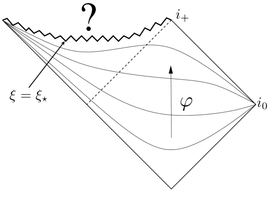
Figure 3: The Penrose diagram of the terminal configuration of a realistic collapse in the khronometric theory. The leaves of constant khronon field are shown by thin solid lines. Non-linear instabilities turn the universal horizon into a singular surface. The structure of the space-time inside this surface can be determined only within the full Hořava gravity.

The physical reason behind the instability of the universal horizon can be understood as follows. As already stated, for the instantaneous signal the universal horizon plays the role of a Cauchy horizon. For an observer falling down the BH and crossing the universal horizon the whole history of the universe outside the BH shrinks into a finite time interval. This leads to an infinite blue-shift of signals sent from the outside, these pile up at the universal horizon and turn it into the singularity. The situation is similar to the instability of the inner Cauchy horizon in the case of Reissner–Nordström and Kerr black holes in GR [34, 35]. However, while in GR the signals destroying the Cauchy horizons are the standard waves propagating along light cones, in the khronometric case they must be instantaneous. Thus the presence of instantaneous interactions plays the crucial role in the destabilization of the universal horizon. Consequently, we expect this type of instability to be absent in the case of the Einstein-aether theory where all modes propagate with finite velocities.

The singularity that replaces the universal horizon is naked in the sense that the complete determination of the khronon field requires imposing some boundary conditions on it. However, for those observers outside the black hole that are able to communicate only using finite-velocity signals (like those interacting only with the ordinary matter) the singularity is hidden by the corresponding sound horizons. Thus, despite the presence of the singularity, the evolution of the ordinary fields can still be unambiguously determined to the extent that their interaction with the khronon can be neglected.

Finally, we do not know if the singularity discussed above is associated with a region of high space-time curvature, or if it is just an irregularity of the khronon foliation. One can conjecture that in the full Hořava gravity the singularity is resolved by the higher order terms, allowing for the complete determination of the dynamics. Admittedly, whether this happens or not is an open issue requiring further study.

5 Discussion

Let us summarize the picture that emerges form our analysis and speculate on its possible implications. It appears that in the healthy Hořava gravity a realistic BH formed as a result of a gravitational collapse has a central region – core – where the preferred foliation and possibly the metric are highly curved. The size of the core is proportional to the Schwarzschild radius with the proportionality coefficient mildly depending on the model parameters. The core appears singular from the point of view of the low-energy khronometric model. Optimistically, one may conjecture that the singularity is resolved once the full structure of the healthy Hořava gravity with the inclusion of higher-derivative terms is taken into account.

The surface of the core can be probed from outside by the high energy modes and by the low-energy instantaneous interactions. In this sense the causal structure of the region outside the core is trivial: the causal horizons appearing for certain modes in the low-energy approximation are absent once the whole spectrum of the theory is considered. Without invoking the full-fledged Hořava gravity it is impossible to tell whether the triviality of the causal structure will persist in the complete solution including the region inside the core. We believe that this is plausible, because the existence of the BH core accessible from the outside would eliminate the threat to BH thermodynamics raised by the violation of Lorentz invariance. Indeed, when considering the gedanken processes of [18, 19] one would also have to take into account the changes in the entropy of the core: in the case of a trivial causal structure these changes are detectable from outside. Though at the moment we cannot estimate the entropy of the core one can speculate that its increase compensates for the decrease of the entropy in the part of the system outside the BH and in this way the second law of thermodynamics is saved.

The existence of the BH core can also have profound consequences on the phenomenon of Hawking radiation. The (in)sensitivity of the latter to trans-Planckian physics is a long-standing issue, see e.g. [36, 37, 38, 39, 40]. Under broad conditions it has been shown that Hawking radiation is determined by the low-energy physics alone, in particular, by the properties of the sound horizons for low-frequency modes [36, 37, 38, 39]. However, a key assumption in these works is that the quantum fields are in the vacuum with respect to the observers freely falling into the BH. This assumption is likely to be violated by the presence of the core just described: on the contrary, it seems more natural to assume that the fields are in the vacuum with respect to the rest frame of the core, which a priori is different from the free-falling one. It would be very interesting to work out what impact this can have on the spectrum of Hawking radiation. An extreme option would be that Hawking radiation gets completely suppressed. Hořava BHs would then behave as stable objects: a kind of ‘dark stars’.

The drastic modification of Hawking radiation is also suggested by the following argument. Consider adding to the healthy Hořava gravity a field carrying a global charge. Imagine that a macroscopically large BH is formed and is endowed with large global charge. It is well-known that if the BH evaporates in the standard manner, the charge conservation will be grossly violated. The immediate way to see this is to note that the standard Hawking radiation is charge-symmetric and thus particles and anti-particles are radiated in equal amounts leaving zero net charge after the BH evaporation. Even allowing for modifications of the radiation introducing a charge asymmetry will not save the day if the radiation remains (approximately) thermal with the temperature of the order of the standard Hawking temperature $T_{H}$. Indeed, the BH starts giving away the charge only when $T_{H}$ exceeds $m$, the mass of the charged particles. Using the standard expression

$$T_{H}\sim M_{P}^{2}/M\;,$$

one estimates the BH mass at this moment

$$M\sim M_{P}^{2}/m\;.$$

Conservation of energy then implies that the charge that can be given back by the BH is bounded above [41, 42] by

$$Q\lesssim M_{P}^{2}/m^{2}\;.$$

On the other hand, the initial charge of the BH can be as large as

$$Q_{0}\sim M_{0}/m\;,$$

where $M_{0}$ is the initial BH mass which, in its turn, can be arbitrarily large. Note that one can further relax the assumption of an approximate thermality of the radiation in the above argument. To show the non-conservation of charge it is sufficient to assume that (a) the BH evaporates and (b) that it cannot emit massive particles during most of its evolution.

The charge non-conservation would prevent Hořava gravity from being a weakly coupled model of quantum gravity. Indeed, consider for concreteness the case when the charge is carried by a scalar field with a global $U(1)$ symmetry. This symmetry is preserved at the perturbative level. Thus any violation of the charge conservation can stem only from non-perturbative gravitational effects. But in a weakly coupled theory, these are expected to be exponentially suppressed [43] meaning that the charge must be conserved, at least with exponential accuracy.

The only way to reconcile BH physics with the charge conservation, and thus save Hořava gravity as a candidate to a consistent quantum theory, is to admit that either even large BHs can emit massive charged particles, or that BHs do not evaporate at all. Clearly, both options would present qualitative departures from the standard picture of Hawking evaporation.

Acknowledgments

We are grateful to Eugeny Babichev, Sergei Dubovsky, Jaume Garriga, Dmitry Gorbunov, Ted Jacobson, Stefano Liberati, Shinji Mukohyama, Oriol Pujolàs, Slava Rychkov, Thomas Sotiriou for illuminating discussions. S.S. thanks the Theoretical Physics Group at IFAE, Barcelona, and the Elementary Particle Theory Group at SISSA, Trieste, for warm hospitality during various stages of this work. We also thank the organizers and participants of the Peyresq 16 Meeting for numerous stimulating conversations. This work was supported in part by the Swiss National Science Foundation, grant IZKOZ2_138892/1 of the International Short Visits Program (D.B.), the Grants of the President of Russian Federation NS-5525.2010.2 and MK-3344.2011.2 (S.S.) and the RFBR grants 11-02-92108, 11-02-01528 (S.S.).

Appendix A Absence of instantaneous propagation in Einstein-aether theory

We have seen in Sec. 2 that the khronometric model exhibits instantaneous interactions. From the mathematical perspective this is due to the fact that the equation describing the khronon is of fourth order because of two extra space-like derivatives. On the other hand, the Einstein-aether theory is described by second-order hyperbolic equations and one does not expect any instantaneous propagation in this case. This seems puzzling as khronon can be viewed as just the restriction of the aether to its longitudinal part. However, this is precisely the restriction that leads to instantaneous signals: in this Appendix we show that in the full aether theory the instantaneous piece is canceled by the transverse modes.

The aether Lagrangian has the form

$${\cal L}_{ae}=-\frac{M^{2}}{2}\Big{[}\alpha(u^{\mu}\nabla_{\mu}u_{\nu})^{2}+\alpha^{\prime}\nabla_{\mu}u_{\nu}\nabla^{\mu}u^{\nu}+\beta\nabla_{\mu}u^{\nu}\nabla_{\nu}u^{\mu}+\lambda(\nabla_{\mu}u^{\mu})^{2}\Big{]}\;.$$ (83)

This differs from the khronon Lagrangian (4) by the presence of the term with the coefficient $\alpha^{\prime}$. The vector $u_{\mu}$ is subject to the unit-norm constraint

$$u_{\mu}u^{\mu}=1\;.$$ (84)

We are interested in the dynamics of perturbations in flat space-time around the background aether configuration

$$\bar{u}_{0}=1~{},~{}~{}~{}~{}\bar{u}_{i}=0\;.$$ (85)

Due to the constraint (84) only space-like components of the aether are excited at the linear level. One separates the perturbations into the longitudinal and transverse parts,

$$u_{i}-\bar{u}_{i}=\partial_{i}\chi+u^{\perp}_{i}~{},~{}~{}~{}~{}\partial_{i}u^{\perp}_{i}=0\;.$$ (86)

The longitudinal part is described by the quadratic khronon Lagrangian (8), where one should make the substitution:

$$\alpha \mapsto\alpha+\alpha^{\prime}\;,$$ (87a)

$$\beta+\lambda \mapsto\beta+\lambda+\alpha^{\prime}\;.$$ (87b)

The Lagrangian for the transverse component is

$${\cal L}_{ae}^{\perp}=\frac{\alpha+\alpha^{\prime}}{2}({\dot{u}}_{i}^{\perp})^{2}-\frac{\alpha^{\prime}}{2}(\partial_{j}u_{i}^{\perp})^{2}\;.$$ (88)

We now introduce coupling of the aether field to the source (10). The contribution of the longitudinal component to the exchange amplitude is given by Eqs. (12), (14) (again with the substitution (87)), and thus contains an instantaneous piece. However, a similar instantaneous contribution, but with the opposite sign, is present in the amplitude describing the exchange of the transverse mode:

$$\begin{split}G^{\perp\;ret}_{ij}(x)&=\int\frac{\mathrm{d}^{4}p}{(2\pi)^{4}}\;\frac{{\rm e}^{-ipx}}{(\alpha+\alpha^{\prime})p_{0}^{2}-\alpha^{\prime}{\bf p^{2}}}\;\bigg{(}\delta_{ij}-\frac{{\bf p}_{i}{\bf p_{j}}}{{\bf p}^{2}}\bigg{)}\\ &=-\frac{\theta(t)\delta(|{\bf x}|-c_{\perp}t)}{4\pi\sqrt{\alpha^{\prime}(\alpha+\alpha^{\prime})}|{\bf x}|}\,\bigg{(}\delta_{ij}-\frac{{\bf x}_{i}{\bf x}_{j}}{|{\bf x}|^{2}}\bigg{)}-\frac{\theta(t)\theta(|{\bf x}|-c_{\perp}t)}{4\pi(\alpha+\alpha^{\prime})}\,\left(\frac{3{\bf x}_{i}{\bf x}_{j}-\delta_{ij}|{\bf x}|^{2}}{|{\bf x}|^{5}}\right)t\;,\end{split}$$ (89)

where $c_{\perp}=\sqrt{\frac{\alpha^{\prime}}{\alpha+\alpha^{\prime}}}$ is the velocity of the transverse mode. The last term in (89) cancels with that in (14) outside the wider sound cone,

$$|{\bf x}|=\max{(c_{\perp},c_{\chi})}\,t\;.$$

Appendix B Spherical solutions: analytic results

In this appendix we present a few analytic results about the solutions of Eq. (38) (or equivalently, the system (36)) with the boundary condition (42) at $\xi=0$.

We begin by proving that if there is a point $\xi_{c}$ where (39) is satisfied, the solution will inevitably cross zero. In other words, all solutions having a sound horizon also possess a universal horizon. Let us assume the opposite. From (41) we observe that the derivative of $U(\xi)$ at the sound horizon is negative,

$$U^{\prime}(\xi_{c})<0\;.$$ (90)

If $U(\xi)$ stays positive at $\xi>\xi_{c}$ at least one of the following conditions must be satisfied:

• there is a point $\xi_{1}>\xi_{c}$ where $U^{\prime}$ first changes sign, i.e. $U^{\prime}(\xi_{1})=0$, $U^{\prime\prime}(\xi_{1})>0$,

• $U(\xi)$ tends to a non-negative constant with $U^{\prime}(\xi)$ asymptotically approaching zero from below; this option implies that $U^{\prime\prime}$ is positive at $\xi\to\infty$.

We proceed to show that none of these two option can be realized. Consider the superluminal case $c_{\chi}\geq 1$. Then it is easy to see that the combination

$$F(\xi)\equiv U^{2}(\xi)(1-c^{2}_{\chi})-1+\xi$$

is positive at $\xi_{c}<\xi<\xi_{1}$. Indeed, this combination vanishes at the sound horizon, while its derivative

$$F^{\prime}=2(1-c^{2}_{\chi})UU^{\prime}+1$$

is positive in the above interval. According to the previous reasoning the factor in front of the square brackets in Eq. (38) is positive at the point $\xi_{1}$, and it is straightforward to see that the quantity in the square brackets is positive as well (recall that $U^{\prime}(\xi_{1})=0$). This implies that $U^{\prime\prime}(\xi_{1})$ is negative and we arrive at a contradiction.

To exclude the option (ii) consider Eq. (38) at large $\xi$. For $U^{\prime\prime}$ to be positive, the combination in the square brackets must be negative. This is possible only if $(U^{\prime})^{2}>C^{2}/\xi\;,$ where $C$ is some constant. This implies $U^{\prime}<-C/\sqrt{\xi}$ and thus $U$ cannot asymptote to a non-negative constant.

It remains to prove the statement in the subluminal case $c_{\chi}<1$. The option (ii) is excluded by the same reasoning as above because the combination $F(\xi)$ is positive at $\xi\to\infty$. However, the option (i) is trickier as it is not possible to argue that $F(\xi)$ is positive in the interval $\xi_{c}<\xi<1$. Thus there may exist a turning point $\xi_{1}$ in this interval. To rule out this possibility we exploit the continuity of the solution in the parameter $c_{\chi}$. If the universal horizon disappears for some values of $c_{\chi}$, there must be a critical value $c_{\chi}^{(1)}$ such that $\xi_{1}$ exists for $c_{\chi}<c_{\chi}^{(1)}$ and does not exist for $c_{\chi}>c_{\chi}^{(1)}$. For $c_{\chi}=c^{(1)}_{\chi}$ the derivative $U^{\prime}(\xi)$ touches zero at $\xi_{1}$,

$$U^{\prime}(\xi_{1})=U^{\prime\prime}(\xi_{1})=0\;.$$

Then from Eq. (38) we obtain $U(\xi_{1})=0$. But this, combined with the requirement $\xi_{1}\leq 1$, implies that the $V$-component of the vector, Eq. (37), is undefined in the vicinity of this point. We have again arrived at a contradiction. This completes the proof.

The system (36) admits analytic solution in two limiting cases: $c_{\chi}=0$ and $c_{\chi}\to\infty$. In the first case Eq. (36a) degenerates into $U^{\prime\prime}=0$ implying that the solution is a linear function,

$$U=1-a\,\xi\;.$$

The constant $a$ is fixed by considering the first approximation in the small velocity $c_{\chi}\ll 1$ and imposing regularity at the sound horizon. In this limit (41) reduces to

$$2U^{\prime}(\xi_{c})U(\xi_{c})=-1.$$

Solving for $\xi_{c}$ from (39) in the same limit and substituting in the previous equation one gets $a=1/2$. This yields the position of the universal horizon in this case,

$$\xi_{\star}\to 2~{}~{}~{}~{}\mathrm{at}~{}~{}~{}~{}c_{\chi}\to 0\;.$$

On the opposite extreme $c_{\chi}\to\infty$ we can neglect the first term in (36a) and obtain the solution

$$V=b\,\xi^{2}~{},~{}~{}~{}~{}U^{2}=1-\xi+b^{2}\xi^{4}\;.$$ (91)

The solution exists at all $\xi$ only if $b\geq b_{0}$, where $b_{0}=\frac{\sqrt{27}}{16}$. In the limit $c_{\chi}\to\infty$ the condition (39) for the position of the sound horizon becomes

$$U(\xi_{c})=0\;.$$

For $b>b_{0}$ the functions $U(\xi)$ corresponding to (91) are strictly positive and thus the solutions do not possess a sound horizon. We believe that these solutions are unphysical and cannot be formed in the gravitational collapse. The physical solution that has a sound horizon corresponds to $b=b_{0}$. The sound horizon in this case is located at $\xi_{c}=4/3$ and coincides with the universal horizon.

References

- [1] T. Jacobson and D. Mattingly, Phys. Rev. D 64, 024028 (2001) [arXiv:gr-qc/0007031].
- [2] T. Jacobson, PoS QG-PH, 020 (2007) [arXiv:0801.1547 [gr-qc]].
- [3] N. Arkani-Hamed, H. C. Cheng, M. A. Luty and S. Mukohyama, JHEP 0405, 074 (2004) [arXiv:hep-th/0312099].
- [4] S. L. Dubovsky, JHEP 0410, 076 (2004) [arXiv:hep-th/0409124].
- [5] V. A. Rubakov and P. G. Tinyakov, Phys. Usp. 51, 759 (2008) [arXiv:0802.4379 [hep-th]].
- [6] S. Groot Nibbelink, M. Pospelov, Phys. Rev. Lett. 94, 081601 (2005). [hep-ph/0404271]. P. A. Bolokhov, S. G. Nibbelink, M. Pospelov, Phys. Rev. D72, 015013 (2005). [hep-ph/0505029].
- [7] O. Pujolas, S. Sibiryakov, “Supersymmetric Aether,” [arXiv:1109.4495 [hep-th]].
- [8] P. Horava, Phys. Rev. D 79, 084008 (2009) [arXiv:0901.3775 [hep-th]].
- [9] K. S. Stelle, Gen. Rel. Grav. 9 (1978) 353.
- [10] D. Blas, O. Pujolas and S. Sibiryakov, JHEP 0910, 029 (2009) [arXiv:0906.3046 [hep-th]].
- [11] D. Blas, O. Pujolas and S. Sibiryakov, JHEP 1104, 018 (2011) [arXiv:1007.3503 [hep-th]].
- [12] D. Blas, O. Pujolas and S. Sibiryakov, Phys. Rev. Lett. 104, 181302 (2010) [arXiv:0909.3525 [hep-th]].
- [13] D. Blas, O. Pujolas and S. Sibiryakov, Phys. Lett. B 688, 350 (2010) [arXiv:0912.0550 [hep-th]].
- [14] T. Jacobson, Phys. Rev. D 81, 101502 (2010) [Erratum-ibid. D 82, 129901 (2010)] [arXiv:1001.4823 [hep-th]].
- [15] D. Blas and H. Sanctuary, Phys. Rev. D 84, 064004 (2011) [arXiv:1105.5149 [gr-qc]].
- [16] D. Blas and S. Sibiryakov, JCAP 1107 (2011) 026 [arXiv:1104.3579 [hep-th]].
- [17] E. Babichev, V. F. Mukhanov and A. Vikman, JHEP 0609, 061 (2006) [arXiv:hep-th/0604075].
- [18] S. L. Dubovsky and S. M. Sibiryakov, Phys. Lett. B 638, 509 (2006) [arXiv:hep-th/0603158].
- [19] C. Eling, B. Z. Foster, T. Jacobson and A. C. Wall, Phys. Rev. D 75, 101502 (2007) [arXiv:hep-th/0702124].
- [20] S. Mukohyama, Open Astron. J. 3, 30-36 (2010). [arXiv:0908.4123 [hep-th]].
- [21] S. Weinberg, “The Quantum theory of fields. Vol. 1: Foundations,” Cambridge, UK: Univ. Pr. (1995)
- [22] C. Eling and T. Jacobson, Class. Quant. Grav. 23, 5643 (2006) [Erratum-ibid. 27, 049802 (2010)] [arXiv:gr-qc/0604088].
- [23] S. Mukohyama, Phys. Rev. D 71, 104019 (2005) [arXiv:hep-th/0502189].
- [24] S. Dubovsky, P. Tinyakov and M. Zaldarriaga, JHEP 0711, 083 (2007) [arXiv:0706.0288 [hep-th]].
- [25] E. Kiritsis, Phys. Rev. D 81, 044009 (2010) [arXiv:0911.3164 [hep-th]].
- [26] E. Barausse, T. Jacobson and T. P. Sotiriou, Phys. Rev. D 83 (2011) 124043 [arXiv:1104.2889 [gr-qc]].
- [27] D. Garfinkle, C. Eling and T. Jacobson, Phys. Rev. D 76, 024003 (2007) [arXiv:gr-qc/0703093].
- [28] G. Gabadadze and L. Grisa, Phys. Lett. B 617, 124 (2005) [arXiv:hep-th/0412332].
- [29] G. Dvali, M. Papucci and M. D. Schwartz, Phys. Rev. Lett. 94, 191602 (2005) [arXiv:hep-th/0501157].
- [30] M. V. Bebronne, Phys. Lett. B 668 (2008) 432 [arXiv:0806.1167 [gr-qc]].
- [31] C. V. Vishveshwara, Phys. Rev. D1 (1970) 2870-2879.
- [32] R. H. Price, Phys. Rev. D5 (1972) 2419-2438; Phys. Rev. D5, 2439-2454 (1972).
- [33] R. M. Wald, J. Math. Phys. 20 (1979) 1056.
- [34] R. A. Matzner, N. Zamorano, V. D. Sandberg, Phys. Rev. D19, 2821-2826 (1979).
- [35] E. Poisson, W. Israel, Phys. Rev. D41 (1990) 1796-1809.
- [36] S. Corley, T. Jacobson, Phys. Rev. D54 (1996) 1568-1586. [hep-th/9601073].
- [37] S. Corley, Phys. Rev. D 57 (1998) 6280 [arXiv:hep-th/9710075].
- [38] W. G. Unruh, R. Schutzhold, Phys. Rev. D71 (2005) 024028. [gr-qc/0408009].
- [39] A. Coutant, R. Parentani, S. Finazzi, “Black hole radiation with short distance dispersion, an analytical S-matrix approach,” [arXiv:1108.1821 [hep-th]].
- [40] C. Barcelo, L. J. Garay, G. Jannes, Phys. Rev. D79 (2009) 024016. [arXiv:0807.4147 [gr-qc]].
- [41] G. Dvali, Fortsch. Phys. 58, 528 (2010) [arXiv:0706.2050 [hep-th]].
- [42] G. Dvali, M. Redi, S. Sibiryakov and A. Vainshtein, Phys. Rev. Lett. 101, 151603 (2008) [arXiv:0804.0769 [hep-th]].
- [43] R. Kallosh, A. D. Linde, D. A. Linde and L. Susskind, Phys. Rev. D 52, 912 (1995) [arXiv:hep-th/9502069].