Testing the accuracy of radiative cooling approximations in SPH simulations

Abstract

Hydrodynamical simulations of star formation have stimulated a need to develop fast and robust algorithms for evaluating radiative cooling. Here we undertake a critical evaluation of what is currently a popular method for prescribing cooling in Smoothed Particle Hydrodynamical (SPH) simulations, i.e. the polytropic cooling due originally to Stamatellos et al. This method uses the local density and potential to estimate the column density and optical depth to each particle and then uses these quantities to evaluate an approximate expression for the net radiative cooling. We evaluate the algorithm by considering both spherical and disc-like systems with analytic density and temperature structures. In spherical systems, the total cooling rate computed by the method is within around $20\%$ for the astrophysically relevant case of opacity dominated by ice grains and is correct to within a factor of order unity for a range of opacity laws. In disc geometry, however, the method systematically under-estimates the cooling by a large factor at all heights in the disc. For the self-gravitating disc studied, we find that the method under-estimates the total cooling rate by a factor of $\sim 200$. This discrepancy may be readily traced to the method’s systematic over-estimate of the disc column density and optical depth, since (being based only on the local density and potential) it does not take into account the low column density route for photon escape normal to the disc plane. We note that the discrepancy quoted above applies in the case that the star’s potential is not included in the column density estimate and that even worse agreement is obtained if the full (star plus disc) potential is employed. These results raise an obvious caution about the method’s use in disc geometry whenever an accurate cooling rate is required, although we note that there are situations where the discrepancies highlighted above may not significantly affect the global outcome of simulations. Finally, we draw attention to our introduction of an analytic self-gravitating disc structure that may be of use in the calibration of future cooling algorithms.

1 Introduction

Star formation simulations require computationally efficient yet robust algorithms for predicting the thermal evolution of the gas during collapse and fragmentation. A cheap and widely used approach (particularly in SPH simulations) is to simply adopt a barotropic equation of state, whose form is motivated by the results of spherical collapse calculations that include a treatment of radiative transfer (Masunaga & Inutsuka, 2000; Larson, 2005). This prescription correctly captures three broad phases of the thermal evolution of the gas, i.e. an isothermal stage at low density followed by successive stages where the gas heats up in response to increasing density. However, by associating gas of a particular density with a corresponding temperature it naturally ignores a variety of effects that in practice will affect the thermal state of the gas (e.g. the geometry, the temperature of the surrounding gas and the local radiation field).

At the other end of the spectrum of complexity, there is a long history of grid based hydrodynamic simulations that follow the thermal evolution of the gas by including energy transfer between the gas and radiation field. Such calculations vary in the level of sophistication with which they model the radiation field, ranging from full frequency dependent radiative transfer (e.g. Wolfire & Cassinelli (1987); Yorke & Sonnhalter (2002)) to the widely employed and cheaper expedient of grey flux limited diffusion (e.g. Bodenheimer et al. (1990); Boley et al. (2007); Boss (2008); Cai et al. (2008); Krumholz et al. (2009)). More recently, several groups have implemented the latter approach within SPH simulations (Whitehouse & Bate, 2004, 2006; Whitehouse et al., 2005; Mayer et al., 2007) and applied this both to large scale star formation simulations (Bate, 2009) and to the fragmentation of self-gravitating discs around young stars (Meru & Bate, 2011). There is however a substantial computational overhead associated with such calculations and this can impose undesirable limitations on the resolution achievable

An intermediate approach is represented by the algorithm proposed by Stamatellos et al. (2007) and developed by Forgan et al. (2009). In its original form, this algorithm (which we henceforth refer to as ‘polytropic cooling’) computed a local cooling rate based purely on local variables. Specifically, it equates the cooling rate per unit mass with the local flux ($F$) divided by the column density ($\Sigma$) of material overlying a particular SPH particle. In the case of optically thin gas that is not subject to external irradiation, this reduces to a cooling rate per unit mass that is simply $\sim\kappa\sigma T^{4}$ (where $\kappa$ is the opacity, $\sigma$ the Stefan Boltzmann constant and $T$ the temperature). This result is correct in the case of non-irradiated optically thin gas in local thermodynamic equilibrium. In the case of optically thick gas in local thermdynamic equilibrium, the correct expression for the cooling rate per unit mass is $\nabla\cdot F/\rho$ where $\rho$ is the local density. As noted above, the polytropic cooling prescription instead sets this to $F/\Sigma$, which is not exactly the same but is likely to be of the same order provided that all quantities (including $F$) vary smoothly over a similar scale length.

In order to calculate $F/\Sigma$ from local variables, the polytropic cooling method makes a further assumption, that it is possible to estimate $\Sigma$ from the local value of the density and potential. In order to achieve this, it is assumed that the relationship between potential ($\Psi$), density (known for each particle in the SPH code) and $\Sigma$ (to be estimated) can be represented by a mass weighted average over an equivalent $n=2$ polytropic sphere in hydrostatic equilibrium. This estimator therefore purely uses the $n=2$ polytrope as a smoothly varying spherical distribution from which one can conveniently make a rough estimate of the relationship between $\rho$, $\Psi$ and $\Sigma$. It does not require that the gas in the simulation is in hydrostatic equilibrium. In fact, the estimated relationship between $\rho$, $\Psi$ and $\Sigma$ (see Appendix) is very similar if one instead bases the mapping on a polytrope of different index, $n$, with the coefficient of $\Sigma$ (Equation 22) varying by around $10\%$ when $n$ is varied over the range $0-5$ (Stamatellos et al., 2007). Evidently, it is the smoothness of the distribution, rather than the specific profile, that is the important property in this mapping procedure. Note that although the rationale for this approximation is based on the structure of smooth spherical distributions (i.e. where all quantities vary over a scale length of order the radius within the sphere) it has also been widely applied in simulations in which discs form and, as such, it is implicitly assumed that this mapping works in planar geometry.

There are several variants of the above algorithm in use. For example, the cooling prescription also usually contains a term that prevents cooling below a background temperature (see Appendix). More recently, a hybrid method has been developed which combines the polytropic cooling method with flux limited diffusion (Forgan et al., 2009). This development follows from the recognition that a possible drawback of the original method is that it always implies cooling of gas (provided that it is hotter than the background temperature), whereas in optically thick regions, the sign of $\nabla\cdot F$ might actually imply that a fluid element is heated by adjoining hotter regions. Flux limited diffusion treats this regime correctly but does not provide a good estimate of the cooling rate per unit mass in regions of low optical depth on the periphery of a condensation. It has been suggested that the advantages of both methods can be combined by simply adding the cooling rates from flux limited diffusion and from polytropic cooling. Clearly this can only be an improvement if each component of the cooling prescription makes a small contribution to the total cooling in the region in which this component is regarded as unreliable. This, however, has not been demonstrated to date.

The development of such approximate cooling prescriptions represents an important opportunity to improve the verisimilitude of star formation simulations at a computational expense that is minimal compared with a full treatment of radiative transfer in the gas. It is obviously important that such prescriptions are rigorously tested. To date, the tests have consisted of modelling the collapse of a $1M_{\odot}$ spherical cloud (Masunaga & Inutsuka, 2000), the simulation of the collapse of a rotating cloud (Boss & Bodenheimer, 1979) and of a self-gravitating disc (Hubeny, 1990) and the thermal relaxation of a static spherical cloud (Spiegel, 1957). In each case, the simulation results have been compared either with previous radiative transfer calculations or else with analytic results. Of these tests, only the latter, known as the Spiegel test, provides a direct measure of the cooling rates. This test (which involves the introduction of sinusoidal temperature variations at a range of wavelengths) demonstrates that polytropic cooling provides a good measure of the cooling rate in the optically thin limit (as indeed it should, given that the cooling rate per unit mass in this limit is independent of the accuracy of the optical depth/column density estimate). However it cannot reproduce the results of this test (for arbitrary temperatute perturbation waevelengths) in the optically thick limit because in this case the cooling rate should depend on the wavelength, as this controls the rate at which radiation diffuses between hotter and colder regions. The polytropic cooling method, however, gives cooling rates that are independent of the wavelength, since this rate is computed only using information about the local temperature and the estimated optical depth to the exterior, rather than on any temperature variations within the structure. The good match to the Spiegel test results in the optically thick limit found by Stamatellos et al. (2007) in fact does not hold if one varies the wavelength from their adopted value. Note that this drawback has been addressed by the hybrid method of Forgan et al. (2009) (which correctly reproduces the results of the Spiegel test in the optically thick limit) since it is able to diffuse heat between hotter and cooler regions.

The other two tests that have been conducted can instead be regarded as ‘macroscopic’ tests inasmuch as they look at the evolution of the entire system. A natural question that arises with such tests is whether their outcomes are as sensitively dependent on a correct treatment of the thermal physics as are the physical situations that will be modelled with the algorithm. This is a hard question to answer unless one has also carried out ‘microscopic’ tests — in other words, an evaluation of the types of situation in which polytropic cooling does (or does not) provide a good estimator of the cooling rate. Once understanding of this question has been gained, one can then examine the physical situations that are encountered in real star formation simulations and decide whether or not the algorithm is likely to be providing a reliable measure of the cooling rate.

With this in mind, we here report on a suite of tests using simple analytic structures in spherical and axisymmetric geometries. We first (§2) compare the predicted values of column density ($\Sigma$) and optical depth ($\tau$) provided by the polytropic cooling method with their true values obtained by integration of the analytic density structures. We then proceed (§3) to compare the polytropic estimate of the cooling rate per unit mass (i.e. $F_{s}/\Sigma$ where $F_{s}$ is the polytropic estimate of the radiative flux) with an equivalent quantity derived using true values of the column density and (in the optically thick limit) compare each of these quantities with what we term the ‘true’ cooling rate; this being related to the divergence of the radiative flux computed in the radiative diffusion approximation. Section 4 summarises our conclusions.

We caution at the outset that such a microscopic examination of the performance of the algorithm is designed to expose its weaknesses and may expose weaknesses which actually turn out to be irrelevant in real simuations. If, for the sake of argument, we find a regime where the method produces cooling rates that are many orders of magnitude different from the true values, this may not actually matter in practice. This is the case if, for example, both true and approximate values lie firmly in the regime where the gas is behaving adiabatically or in a regime where the gas temperature is controlled by the ambient cloud temperature. Here we simply present our results in order that those who use this method in hydrodynamical simulations can assess the significance in practice of the discrepancies that we highlight here.

2 Comparison of column density and optical depth estimates

2.1 The application of the polytropic method to spherical hydrostatic structures

We set up a set of simple model density and temperature distributions corresponding to various polytropes in hydrostatic equilibrium. Hydrostatic structures are of interest when testing the radiative cooling approximation since these systems will, once formed, tend to exist for prolonged periods in hydrodynamical simulations and their thermal evolution in a given state will be important as well as their dynamical evolution.

Given an assumed dependence of the Rosseland mean opacity on density and temperature, we can readily compute the column density ($\Sigma$) and optical depth ($\tau$) along a radial path from any given point to infinity. We then compare these quantities t the column densities and optical depths predicted by the polytropic cooling method ($\Sigma_{poly}$ and $\tau_{poly}$; see Appendix). We emphasise that $\tau_{poly}$ is not simply the product of the local opacity and the estimated column density but also contains a (opacity law dependent) factor that estimates the ratio of local opacity to the path averaged opacity within the polytropic smoothing formulation; see Stamatellos et al. (2007) and Appendix A.4. This aspect of the polytropic cooling formulation is designed to improve the optical depth estimate in cases where the opacity is a strongly varying function of temperature (and hence position) as in the so-called ‘opacity gap’ in protostellar discs.

It is worth noting some features of the approximation that will be useful in interpreting our results. Members of a polytropic family of given $n$ can all be mapped onto a single function representing the dependence of a scaled density-like variable on a scaled radius variable ($\xi$). The polytropic cooling approximation first assumes that a given particle corresponds to a particular value of $\xi$ within a polytropic sphere and then, given the actual values of density and potential at that particle, determines the corresponding value that the column density would have in that case. This is repeated over a range of $\xi$ values and then a final ‘effective’ column density is computed which weights the contributions from different $\xi$ in proportion to the amount of mass at different $\xi$ values within the polytropic sphere. Since for an $n=2$ polytrope, the majority of the mass is located at rather large radii (see Figure 1), this implies that the relationship between $\Psi$, $\rho$ and $\Sigma$ is equivalent to assuming that the particle resides towards the outskirts of a structure. It therefore implies a lower value of $\Sigma$ (for fixed $\Psi$ and $\rho$) than for a particle that was mapped onto the centre of a polytropic sphere. The polytropic cooling method applies this weighting over $\xi$ to all particles since, being entirely local, it has no knowledge of where any particular particle is located within a parent structure. Therefore if, in fact, a particle is close to the core of its parent structure, the weighting of the polytropic cooling method will systematicallly underestimate the overlying column density. Conversely, for particles in the extreme periphery of a structure, the weighting of the polytropic method over-estimates the column density at given $\Psi$ and $\rho$.

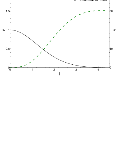
Figure 1: Density profile and cumulative mass distribution for the $n=2$ polytrope (in arbitrary units) which is the basis for the mapping between $\rho$, $\Psi$ and $\Sigma$ in the polytropic cooling method. Note that the mass distribution is weighted towards larger radius.

This simple insight is sufficient for us to understand the method’s systematic under-estimate of the column density near the centre of spherical structures and, conversely, its systematic over-estimate in the outer regions (Figure 2). The method under-estimates the central column density by about a factor three for all polytropic spherical structures and the over-estimate at large radius is around a factor three for polytropes with $n$ of $2$ or greater and larger for smaller $n$ (less compressible gas).

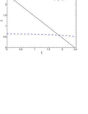
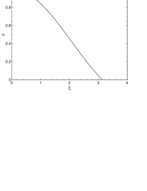
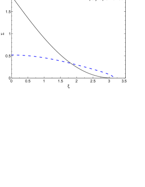
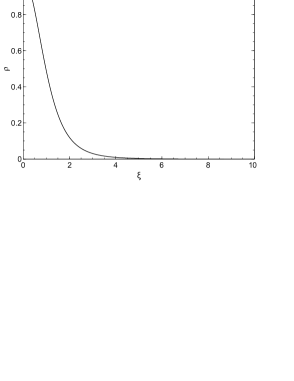
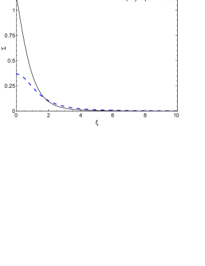
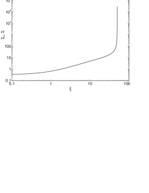
Figure 2: Algorithm tests for spherical polytropes. Upper row: $n=0$ (uniform density), middle row: $n=1$ polytrope, lower row: $n=5$ (nearly isothermal) polytrope. In each case, the left hand panel is the density profile, the middle panel compares the integrated column density to infinity from each point (solid line) with the corresponding quantity derived by the polytropic cooling method (dashed line) and the right hand panel is the ratio of values for the column density on a logarithmic scale. Units are arbitrary.

In the case of constant opacity (e.g. that due to electron scattering), these results for the column density apply directly to the derived optical depth since the two quantities are simply proportional. In Figure 3 we present the optical depth as a function of radius for the case of opacity given by ice grains for which $\kappa\propto T^{2}$. Note that normalisation of optical depth is arbitrary. This illustrates that within the region containing the bulk of the mass, the polytropic method underestimates the optical depth.

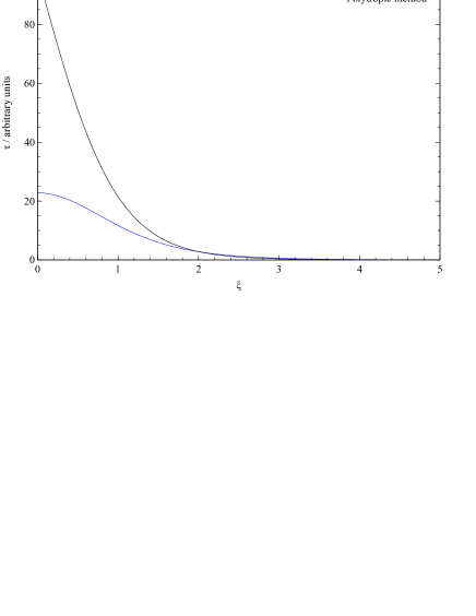
Figure 3: Comparison of the optical depth (in arbitrary units) due to ice and the polytropic estimate of the same quantity (dashed line) in the case of the $n=4$ polytrope. Note that the normalisation for the optical depth is arbitrary.

2.2 The application of the polytropic method to disc-like geometries

We test the polytropic method in planar geometry, being mindful of the fact that this applies to a number of situations that occur in hydrodynamical simulations such as shock compressed sheets and rotationally supported discs. To this end we use an approximately Keplerian disc model in which both the column density ($\Sigma$) and vertically averaged temperature vary as $R^{-3}$. Such a structure has a radially constant profile of Toomre $Q$ parameter (Toomre, 1964) as would be expected in the case of discs that are in a state of self-regulated marginal stability against self-gravity (Gammie et al., 2000; Rice et al., 2003). In fact, this particular profile corresponds to the case of a disc with constant accretion rate and radiative cooling with opacity provided by ice grains (Clarke, 2009), an opacity regime that is applicable to the outer regions of discs around young stars and where the cooling rate is important in determining whether such discs fragment.

Although (as emphasised by Stamatellos et al 2007), their cooling prescription is not only applicable to situations that are in hydrostatic equilibrium, we here test the method on a density and temperature field that most closely resembles the situations that arise in star formation simulations in which hydrostatic equilibrium normal to the disc plane is attained on a short (dynamical) timescale (we assume that the small influence of pressure gradients and of the disc’s self-gravity in the disc plane is balanced by a minor adjustment of the disc’s rotation curve). In order to obtain an analytic approximation to the disc vertical structure as a function of radius, we approximate the vertical gravitational acceleration at height $z$ in the disc as

$$g_{z}=-\Omega^{2}z-4\pi G\Sigma^{\prime}$$ (1)

where the first term is the vertical component of the gravitational acceleration provided by the central star ($\Omega$ is the local Keplerian angular velocity) and $\Sigma^{\prime}$ is the column density between the point at height z and the disc mid-plane (which is not to be confused with the column density to infinity that has been discussed hitherto). This second term is the gravitational acceleration that the disc would exert in the limit that it was an infinitely extended stratified slab. In reality there are further small corrections to the self-gravity due to radial gradients in the disc (see e.g. the appendix of Bertin & Lodato, 1999). We have verified a posteriori (by subtracting the density distribution of a radially constant disc from the computed structure and then calculating $g_{z}$ by direct summation) that this further correction would account for at most $\sim 3\%$ of the total $g_{z}$ value. We emphasise that this approximate $g_{z}$ value is only used in order to obtain a structure that is in approximate vertical hydrostatic equilibrium and that the full disc (and star) potential is used when computing the polytropic cooling.

The motivation for adopting this approximate form of $g_{z}$ is that it allows us to compute an analytic disc structure as a function of cylindrical radius ($R$) and z, since such a disc can be modeled by an $n=2$ polytrope with $P=K\rho^{2}$ where $K$ is a global constant. In this case, differentiation with respect to $z$ of the hydrostatic equilibrium equation normal to the mid-plane yields the modified simple harmonic equation:

$${{\partial^{2}\rho}\over{\partial z^{2}}}=-{{2\pi G}\over{K}}\bigl{(}\rho+{{\Omega^{2}}\over{4\pi G}}\biggr{)}$$ (2)

whose solution (subject to $\rho=\rho_{0}$ and $\rho^{\prime}=0$ at $z=0$) is

$$\rho=\rho_{0}\biggl{(}\bigl{(}1+f(Q)\bigr{)}{\rm cos}{{z}\over{H_{0}}}-f(Q)\biggr{)}$$ (3)

where

$$f(Q)={{\Omega^{2}}\over{4\pi G\rho_{0}}}$$ (4)

and

$$H_{0}=\biggl{(}{{K}\over{2\pi G}}\biggr{)}^{1/2}$$ (5)

The constant $f$ is of order $Q$ when $Q\gg 1$ (the non-self gravitating case) while $f\sim Q^{2}$ in the strongly self-gravitating case ($Q\ll 1$). In the marginally self-gravitating (self-regulated) case that we consider here, $f$ is of order unity.

The density profile given above allows us to derive the scale height of the disc (defined here as being the height at which the density falls to zero):

$$H=H_{0}{\rm cos}^{-1}\biggl{(}{{f(Q)}\over{1+f(Q)}}\biggr{)}$$ (6)

We set up such a disc over the radial range $R=1$ to $R=10$ (in arbitrary units), and adopt parameters $f=1$ and $H_{0}=0.35$. For this model the total disc mass (which, given the surface density profile, is concentrated at small radii) is $\sim 20\%$ of the central star mass. At given $R$ and $z$, we compute the gravitational potential by adding the contributions due to the star and the rest of the disc. The latter is calculated by using elliptic integrals to compute the contribution to the potential from each ring of material corresponding to each pair of $R$ and $z$ values in the grid. The local density and potential is then used to obtain the polytropic cooling method’s estimator of the column density which is compared with the ‘true’ column density integrated out to infinity in the $z$ direction. Figure 4 compares these column density values as a function of $z$ for a cylindrical slice at $R=5$, at which point the disc aspect ratio $H/R\sim 0.07$. The upper curve in the Figure represents the case that the full (star plus disc) potential is used in the estimation of $\Sigma$, whereas the intermediate curve uses just the disc potential (an approach suggested by Stamatellos et al 2007 though not always implemented in disc studies). As expected, the estimated column density is larger when the stellar potential is included by around a factor $2\sim 3$, consistent with the square root dependence of the estimated column density on the potential and the fact that the disc mass is concentrated towards the inner part of the disc. However, even in the case that only the disc potential is included, the estimated column density exceeds the true column density by a factor 5 or more at all heights. The consistent sign of the discrepancy (in the sense that the estimated column is always larger) is simply because in a disc geometry there is always a low column density route to infinity (along the symmetry axis) which is not accounted for by the estimated value.

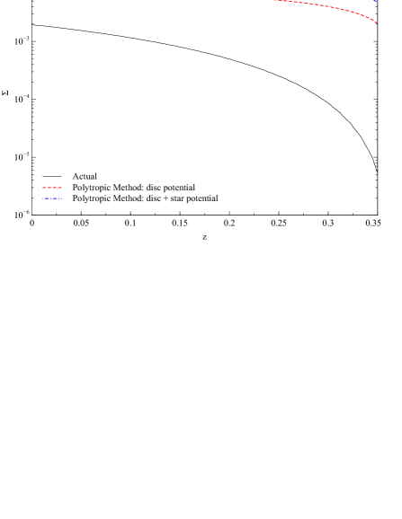
Figure 4: The column density in the $z$ direction out to infinity in disc geometry, compared to the polytropic estimate.

2.3 Summary

We find that in the case of spherical structures, the polytropic method under-estimates the column density (and hence optical depth in the case of constant opacity discs) by a factor of $3\sim 4$ in the inner regions and over-estimates the column density at large radius. This can be understood in terms of the weighting function that is used in order to map the density and potential onto the column density which is weighted towards the relationship between these quantities that applies at intermediate radii within an $n=2$ polytrope.

On the other hand, the method systematically over-estimates the (vertical) column density in a disc structure, even in the case that one uses only the potential from the disc (rather than the disc plus star) in estimating the column density. For the disc structure we have modeled (for which $H/R\sim 0.07$ at the radius considered and where $Q_{T}\sim 1$ throughout), this over-estimate is around a factor $5$ or more. This over-estimate can be understood as a geometric effect in that the estimate based on local density and potential does not take account of the direction of low $\Sigma$ normal to the disc plane.

3 Implications of results for the estimate of cooling rates

The polytropic method uses the column density and optical depth estimates discussed above to compute the cooling rate per unit mass according to

$$\dot{U}=\frac{\sigma T^{4}-\sigma T_{0}^{4}}{\bigl{(}\tau+\tilde{\tau}^{-1}\bigr{)}\Sigma}$$ (7)

Here, $\tau$ is the path averaged optical depth (see Appendix A.3) whereas $\tilde{\tau}$ is the product of local opacity and estimated column density. These two quantities differ by a factor that is usually of order unity, except in regions where the opacity is strongly dependent on temperature (see Figure 6 of Stamatellos et al., 2007). Note that in both cases the opacity is given by parametrisations of the Rosseland mean opacity

There are several approximations involved in Equation 7. First of all, it is assumed that the cooling rate per unit mass at a given point is simply an estimator of the local radiative flux divided by the estimated column of material above this point. Secondly, it takes a form for the local radiative flux designed to have particular functional forms in the limits of small and large optical depths. At low optical depths this is simply the product of the optical depth and the black body flux. In the limit of large optical depth, this expression is motivated by the radiative diffusion approximation

$$F=-{{4}\over{3\kappa\rho}}\nabla(\sigma T^{4})$$ (8)

and is likely to be of similar order to Equation 8, provided that all quantities vary over a scale length $r$ (so that $\frac{T^{4}}{\tau}\sim\frac{dT^{4}}{d\tau}$). Finally, the second term in the numerator of Equation 7 ensures that the cooling rate goes to zero at temperature $T_{0}$ and is designed to mimic the effect of an external radiation field at this temperature. For the purposes of the test we set $T_{0}=0$.

However, it is important to recognise that Equation 7 is itself an approximation. In the optically thick limit we can also evaluate the ‘true’ cooling rate per unit mass, using

$$\dot{U}_{thick}={{1}\over{\rho}}\nabla\cdot F$$ (9)

where $F$ is evaluated in the diffusion limit (i.e. Equation 8).

3.1 Cooling rates in spherical geometry

We first examine how the cooling values predicted by Equation 7 using column density and optical depths estimated by the polytropic method compares with the same quantity evaluated using the actual optical depths and column densities. In each figure, the left hand panel refers to the case of constant opacity and the right hand panel to the case $\kappa\propto T^{2}$. For the purpose of this comparison, we evaluate the temperature profile (Figure 5) by assuming that the structure is in hydrostatic equilibrium. The (true) optical depth to the centre is $42$ for the constant opacity case and 100 for the case of ice and the point at which the (true) optical depth is unity is marked by the arrow in Figure 6.

Figure 5: Density (left panel) and temperature (right panel) profiles, in arbitrary units, of the hydrostatic $n=4$ polytrope used for the cooling rate comparisons.

Figure 6 shows that the polytropic cooling estimate of Equation 7 (black line) has the same general shape as the same quantity evaluated from the actual column density (green dotted line), in that in both cases the cooling rate per unit mass is highest close to an optical depth of unity and that both converge to the same value in the limit of low optical depth. This is to be expected since as $\tau$ tends to zero, the cooling rate per unit mass tends to a value that is independent of column density and depends only on temperature (the optically thin limit of Equation 7 is shown by the blue dash-dot line in Figure 6). However, in the optically thick portion of the disc, the two cooling rates are in general quite different, with the polytropic estimate over-estimating the cooling at small radii and under-estimating it at large radii. This can be simply understood in that the cooling rate per unit mass in the optically thick limit scales as $1/\Sigma^{2}$ and hence this result reflects the respective under-estimate and over-estimate of $\Sigma$ at small and large radius.

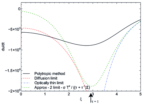
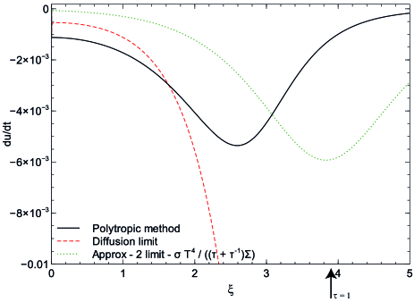
Figure 6: Comparison of estimates of the cooling rate per unit mass (in arbitrary units) for the case of a) constant opacity and b) ice grain opacity for $n=4$ polytropic spheres with (true) central optical depths of $42$ and $100$, respectively. The black line represents the polytropic estimate to Equation 7 while the green dotted line uses the same equation but with the true values of the optical depth and column density. The blue dash-dot line is the limiting form of both expressions at low optical depth where they agree by construction. The red dashed line is the ‘true’ cooling rate computed using the radiative diffusion approximation (Equations 8 and 9). The arrows denote the point of (true) optical depth equal to unity.

So far, we have just examined how the accuracy of estimating the column density affects the cooling rate as specified by Equation 7. A more important comparison is however the comparison of the polytropic method’s estimated cooling rate with the ‘true’ (radiative diffusion) method in the limit of high optical depth (Equations 8 and 9), shown as the dashed red line in Figure 6. Interestingly, this agrees rather well with the polytropic method in the optically thick region (the black line) in both opacity regimes. In both cases the total (mass integrated) cooling rates agree to within a few tens of per cent. Such a discrepancy is almost certainly no larger than additional errors due to poorly determined opacities, for example. We have also explored a variety of different polytropic spherical structures and different opacity laws and find that the polytropic cooling method’s fair (i.e. order unity) agreement with the results of radiative diffusion is reproduced for a wide range of input parameters. This explains why the method performed well in reproducing the results of the spherical collapse calculation of Masunaga & Inutsuka (2000).

When the cooling rates are integrated over mass through the optically thick part of the structure, one obtains the result that the polytropic method modestly under-estimates the total cooling rate by around $20\%$ (compared to the radiative diffusion limit) in both cases. The switch in the sign of the discrepancy at intermediate radius means that the global values agree rather well despite the discrepancies in local rates.

It is perhaps surprising that the polytropic cooling method reproduces the ‘true’ (radiative diffusion) cooling rate considerably better than it reproduces the quantity that it ostensibly computes (Equation 7). This is because Equation 7 is only a reasonable approximation of Equation 8 in the case that one can replace differentiation with respect to $\tau$ by simple division by $\tau$. Comparison between the green and red lines in Figure 6 show that this is a poor approximation at small radius, i.e. the temperature falls over an optical depth that is a small fraction of the total optical depth at small radius and hence simple division by $\tau$ under-estimates the magnitude of the cooling. This is almost exactly compensated by the fact that the polytropic cooling method under-estimates the optical depth in the central regions (see §2). Although it may be regarded as unfortunate that the reason for this good agreement is a near cancellation of discrepancies of comparable magnitude, we are encouraged that, as described above, the reasonable agreement appears to hold - in spherical geometry for a wide range of input parameters.

3.2 Cooling rates in disc geometry

The situation in disc geometries is very different. As above, we start by comparing the polytropic cooling estimate of Equation 7 with the same quantity evaluated using the true column density at each point. For consistency with the cooling regime encountered in the outer regions of self-gravitating discs, we employ the opacity appropriate to ice cooling ($\kappa\propto T^{2}$). We here focus on the optically thick regions of the disc, in order to allow comparison with Equation 8 and so neglect the additive term $\propto\tilde{\tau}^{-1}$ in the denominator of Equation 7. Figure 7 plots the specific cooling rate estimates as a function of $z$ for the slice at $R=5$ in the model disc described in §2.2. The dashed line represents the cooling rate according to the radiative diffusion approximation (i.e. Equations 8 and 9) while the upper solid line employs Equation 7 where the column density is the ‘real’ value and the optical depth is approximated as the product of the real column density and the local opacity. The lower two lines correspond to Equation 7 evaluated according to the polytropic method where the optical depth is the product of the estimated column density and the estimated average opacity along the line of sight (see Appendix A.4). In the case $\kappa\propto T^{2}$ this is $0.58$ times the local opacity. The bottom line uses the full (star plus disc) potential in estimating the column density whereas the curve above uses the disc potential only.

Recalling that in the optically thick regime the, cooling rate according to Equation 7 scales as $\Sigma^{-2}$ and that the method over-estimates the column density in disc geometries, it is no surprise that now the polytropic cooling method yields a much smaller cooling rate, being at least an order of magnitude lower in the case that only the disc potential is applied and more than two orders of magnitude if the total (star plus disc) potential is used.

When we compare each of these rates with the ‘true’ cooling rate in the radiative diffusion approximation (dashed curve, Equation 8) we find that the latter is now of comparable magnitude to the cooling computed from Equation 7 using the true column density but is far larger than the estimates from polytropic cooling. Thus in contrast to the case in spherical geometry, there is no compensating effect that brings the polytropic estimate into agreement with the ‘true’ cooling rate.

Figure 8 illustrates how the specific cooling rates that are compared in Figure 7 affect the total cooling rate per unit area. At each value of $z$, the quantity plotted is given by the integral of the product of specific cooling rate and density from $z^{\prime}=0$ to $z$. Note that in contrast to Figure 7, Figure 8 is plotted on a linear scale. It illustrates that at all heights, the use of Equation 7 gives a reasonable (order unity) estimate of the integrated cooling rate provided one has knowledge of the ‘true’ column density. Indeed, the total cooling rate per unit area is within $25\%$ of the result of using the radiative diffusion approximation. The total cooling rate from the polytropic method is, however, too low by a factor of at least $\sim 200$. This emphasises that, in disc geometry, the most pressing problem is to find a reliable estimator of the column density.

We have also experimented with varying the opacity law in the disc geometry and note that when the opacity is a less strongly increasing function of temperature, there is a greater tendency (compared with the spherical case) for discs to be in the regime of net heating (i.e. the upper regions receive a greater flux from the warm disc below than they radiate upwards — the outwardly increasing area element in spherical geometry makes this less likely in the spherical case). Obviously, no local cooling prescription can reproduce this effect. Thus any future efforts to find an improved local cooling prescription in disc geometries will need to be carefully calibrated in different opacity regimes.

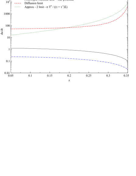
Figure 7: The cooling rate for the disc system evaluated by the polytropic cooling method (both including and excluding the stellar potential) compared with the diffusion limit as well as Equation 7 using analytic optical depths at radius $R=15$.

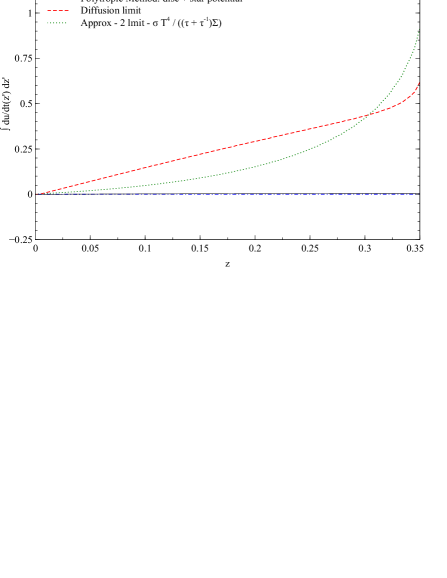
Figure 8: Magnitude of the integrated cooling rate per unit area for the disc evaluated by the polytropic cooling method compared with the diffusion limit as well as Equation 7 using analytic optical depths at radius $R=15$.

4 Conclusions

The polytropic method works quite well in spherical geometry. We have shown that over a wide range of input parameters the mass integrated cooling rate out to the $\tau=1$ surface matches that from radiative diffusion to within order unity or better, an error that is probably negligible compared with other uncertainties such as those in the opacities. This good agreement is ‘fortuitous’ in the sense that it results from two nearly compensating discrepancies, but can nevertheless be exploited in simulations in spherical symmetry.

The polytropic cooling estimate, however, performs poorly in optically thick discs, regardless of whether one uses the potential from the disc alone or that due to the star and the disc in order to estimate the column density. This is due to the fact that the polytropic method over-estimates the column density considerably (§2) since it does not take account of the lower column density route normal to the disc plane. This translates into an under-estimate of the cooling rate by between two and three orders of magnitude (Figures 7 and 8), depending on whether the stellar potential is included in the column density estimate. We have shown however that (at least in the astrophysically relevant ice opacity regime) the cooling can be well modelled in disc geometries if only one can improve the column density estimate. This should clearly motivate further algorithmic developments in this area.

The above is sufficient to say that the method needs to be used with caution, though it does not necessarily negate results in the literature that use this method. For example, the outer regions of proto-stellar discs may in fact be nearly isothermal at the back-ground temperature, in which case all methods would agree on the thermal structure of the disc. Alternatively, even if simulations enter regimes where the cooling rate is strongly under-estimated, it may have a negligible effect on where, for example, fragmentation occurs in the disc. This is because the cooling rate in such discs is a very strong function of radius (Clarke, 2009) and thus an under-estimate in cooling would cause only a modest increase in the radius at which the disc fragments.

Simulators evidently need to balance these issues against the computational economies offered by polytropic cooling. These results can also inform those wishing to combine polytropic cooling with other methods, for example the expedient of adding the polytropic cooling method to flux limited diffusion (as in the ‘hybrid’ method of Forgan et al) relies on the former being a minority contributor in the optically thick regions where the latter is correct. We find that this requirement is amply fulfilled. On the other hand, whether or not the hybrid is an improvement over pure flux limited diffusion depends on the situation. Unlike the flux limited diffusion method, the hybrid method would yield the correct cooling rate for non-irradiated optically thin gas. Neither method, however, is suitable for treating the optically thin regions above an optically thick disc which are subject to irradiation from the disc below. Whether or not this matters for the system dynamics obviously depends on the topic at hand.

Finally, we draw attention to the fact that an astrophysically relevant disc structure (a marginally self-gravitating optically thick steady state disc with opacity dominated by ice grains) can be modelled as an $n=2$ polytrope whose density and temperature structure can be described analytically. The existence of such an analytic solution may be useful in testing future cooling algorithms.

Appendix A The Polytropic Cooling Method

The radiative cooling of an element within a cloud is determined by the optical depth of that point, that is the integrated opacity along the line-of-sight out of the cloud. The polytropic cooling method of Stamatellos et al. (2007) aims to evaluate the radiative cooling of an element by calculating an approximate optical depth using only local variables at the point of interest.

In order to achieve this, the particle of interest is taken to be embedded at an arbitrary position in a spherically symmetric pseudo-cloud, modelled by a polytrope of index $n$. The density ($\rho$), potential ($\Psi$) and temperature ($T$) of the polytrope are given by the solutions of the Lane Emden equation, $\theta_{n}$,

$$\rho(\xi) = \rho_{c}\theta^{n}(\xi)$$ (10)

$$\Psi(\xi) = -4\pi GR_{0}^{2}\rho_{c}\phi(\xi)$$ (11)

$$T(\xi) = T_{c}\theta(\xi)$$ (12)

where $\phi(\xi)=-\xi_{B}\left(\frac{d\theta}{d\xi^{\prime}}\right)_{\xi^{\prime}=\xi_{B}}+\theta(\xi)$.

The parameters of the polytrope are set to reproduce the local conditions at the location of the particle. The column density, optical depth and radiative cooling are then calculated for the particle embedded in the pseudo-cloud. The value of the column density to the particle of interest is taken to be the average column density over all possible positions within the pseudo-cloud.

A.1 Calibrating the Pseudo-Cloud

Once the polytropic index of the barometric equation of state is set, the values of the central density, scale length and core temperature for the pseudo-cloud in which the particle of interested is embedded at a radius $r=R_{0}\xi$ are calculated such that the known density ($\rho_{i}$), gravitational potential ($\Psi_{i}$) and temperature ($T_{i}$) at the position of the particle are reproduced.

$$\rho_{c} = \rho_{i}\theta^{-n}(\xi)$$ (13)

$$R_{0} = \sqrt{\frac{-\Psi_{i}\theta^{n}(\xi)}{4\pi G\rho_{i}\phi(\xi)}}$$ (14)

$$T_{c} = T_{i}\theta^{-1}(\xi)$$ (15)

A.2 Column Density

The column density (mass per unit area along a line-of-sight) from a particle at radius $r=\xi R_{0}$ along a radial line to the edge of the pseudo-cloud ($\xi=\xi_{B}$) is given by

$$\Sigma=\int_{r}^{r_{B}}\rho(r)dr=R_{0}\int_{\xi}^{\xi_{B}}\rho(\xi^{\prime})d\xi^{\prime}$$ (16)

Substituting for the density using Equation 10,

$$\Sigma(\xi)=R_{0}\int_{\xi}^{\xi_{B}}\rho_{c}\theta^{n}(\xi^{\prime})d\xi^{\prime}$$ (17)

And substituting for $\rho_{c}$ and $R_{0}$ using Equations 13 and 14,

$$\Sigma(\xi)=\sqrt{\frac{-\Psi_{i}\rho_{i}}{4\pi G\phi(\xi)\theta^{n}(\xi)}}\int_{\xi}^{\xi_{B}}\theta^{n}(\xi^{\prime})d\xi^{\prime}$$ (18)

When calculating the mean column density over all positions of the particle within the pseudo-cloud, the column density at a given radius $\Sigma(\xi)$ is weighted by the mass contained in a spherical shell radius $\xi$ thickness $d\xi$, $M(\xi)$ as this gives the probability of the particle being within that shell. The total mass of the cloud, $M$ is used to normalise the distribution.

$$\bar{\Sigma}=\frac{1}{M}\int_{0}^{\xi_{B}}\Sigma(\xi)M(\xi)d\xi$$ (19)

The mass enclosed in a spherical shell is given by the volume of the shell multiplied by the density, from the Lane-Emden function, $M(\xi)=4\pi R_{0}^{3}\rho_{c}\xi^{2}\theta^{n}(\xi)$. The total mass of the cloud is $M=\int_{0}^{\xi_{B}}4\pi R_{0}^{3}\rho_{c}\xi^{2}\theta^{n}(\xi)d\xi$.

Substituting these in to the integral gives

$$\bar{\Sigma}=\left[\int_{0}^{\xi_{B}}\xi^{2}\theta^{n}(\xi)d\xi\right]^{-1}\int_{0}^{\xi_{B}}\xi^{2}\Sigma(\xi)\theta^{n}(\xi)d\xi$$ (20)

Evaluating the first integral and substituting in the column density,

$$\bar{\Sigma}=\left[-\xi_{B}^{2}\left(\frac{d\theta}{d\xi}\right)_{\xi=\xi_{B}}\right]^{-1}\int_{0}^{\xi_{B}}\left[\int_{\xi}^{\xi_{B}}\theta^{n}(\xi^{\prime})d\xi^{\prime}\right]\sqrt{\frac{-\Psi_{i}\rho_{i}\theta^{n}(\xi)}{4\pi G\phi(\xi)}}\xi^{2}d\xi$$ (21)

Which can be written

$$\bar{\Sigma}=\zeta_{n}\sqrt{\frac{-\Psi_{i}\rho_{i}}{4\pi G}}$$ (22)

Where $\zeta_{n}$ is just a constant for a given polytropic index.

$$\zeta_{n}=\left[-\xi_{B}^{2}\left(\frac{d\theta}{d\xi}\right)_{\xi=\xi_{B}}\right]^{-1}\int_{0}^{\xi_{B}}\left[\int_{\xi}^{\xi_{B}}\theta^{n}(\xi^{\prime})d\xi^{\prime}\right]\sqrt{\frac{\theta^{n}(\xi)}{\phi(\xi)}}\xi^{2}d\xi$$

Values of $\zeta_{n}$ can be evaluated numerically and are given in Table 1. It can be seen that the results for the column density are fairly insensitive to the polytropic index chosen in the approximation.

$n$	$\zeta_{n}$
0.0	0.3796
1.0	0.3756
2.0	0.3682
3.0	0.3600
4.0	0.3500
5.0	0.3322

Table 1: Values of $\zeta_{n}$ for different polytropic indices (evaluated numerically).

This mean is used as the approximate value of the column density at the point in question and depends only on the local potential and density. In this formula, the local potential conveys the structure of the surrounding space (rather than performing the integral along the line-of-sight).

A.3 Optical Depth

The optical depth along a ray path with absorption coefficient $\alpha_{u}$ is defined as $\tau_{u}=\int\alpha_{u}(r)dr$ with $\alpha_{u}=\kappa_{u}\rho$. This can be averaged over all frequencies in the black body spectrum using the Rosseland-mean opacity $\kappa_{R}(\rho,T)$.

The optical depth of a particle at radius $r=\xi R_{0}$ in the pseudo-cloud can be calculated,

$$\tau(\xi)=\int_{\xi}^{\xi_{B}}\kappa_{R}(\rho(\xi^{\prime}),T(\xi^{\prime}))\rho(\xi^{\prime})R_{0}d\xi^{\prime}$$ (23)

Substituting for the density and temperature using Equations 10 and 12,

$$\tau(\xi)=\int_{\xi}^{\xi_{B}}\kappa_{R}(\rho_{c}\theta^{n}(\xi^{\prime}),T_{c}\theta(\xi^{\prime}))\rho_{c}\theta^{n}(\xi^{\prime})R_{0}d\xi^{\prime}$$ (24)

And substituting for $\rho_{c}$, $T_{c}$ and $R_{0}$ using Equations 13, 14 and 15,

$$\tau(\xi)=\sqrt{\frac{-\Psi\rho_{i}\theta^{n}(\xi)}{4\pi G\phi(\xi)}}\int_{\xi}^{\xi_{B}}\kappa_{R}\left(\rho_{i}\left[\frac{\theta(\xi^{\prime})}{\theta(\xi)}\right]^{n},T_{i}\left[\frac{\theta(\xi^{\prime})}{\theta(\xi)}\right]\right)\left[\frac{\theta(\xi^{\prime})}{\theta(\xi)}\right]^{n}d\xi^{\prime}$$ (25)

The mass-weighted pseudo-mean optical depth (averaging over all possible positions of the particle within the pseudo-cloud) can be obtained as for the column density.

$$\bar{\tau} = \left[-\xi_{B}\left(\frac{d\theta}{d\xi^{\prime}}\right)_{\xi^{\prime}=\xi_{B}}\right]^{-1}\int_{0}^{\xi_{B}}\xi^{2}\tau(\xi)\theta^{n}(\xi)d\xi$$

$$\bar{\tau} = \left[-\xi_{B}\left(\frac{d\theta}{d\xi^{\prime}}\right)_{\xi^{\prime}=\xi_{B}}\right]^{-1}\sqrt{\frac{-\Psi_{i}\rho_{i}}{4\pi G}}$$

$$\int_{0}^{\xi_{B}}\left[\int_{\xi}^{\xi_{B}}\kappa_{R}\left(\rho_{i}\left[\frac{\theta(\xi^{\prime})}{\theta(\xi)}\right]^{n},T_{i}\left[\frac{\theta(\xi^{\prime})}{\theta(\xi)}\right]\right)\theta^{n}(\xi^{\prime})d\xi^{\prime}\right]$$

$$\sqrt{\frac{\theta^{n}(\xi)}{\phi(\xi)}}\xi^{2}d\xi$$

A.4 Pseudo-Mean Mass Opacity

Once the column density and optical depth have been calculated, one can define an average opacity along the line-of-sight,

$$\bar{\kappa} = \frac{\bar{\tau}}{\bar{\Sigma}}$$

$$\bar{\kappa}(\rho,T) = \left[-\zeta_{n}\xi_{B}\left(\frac{d\theta}{d\xi^{\prime}}\right)_{\xi^{\prime}=\xi_{B}}\right]^{-1}$$

$$\int_{0}^{\xi_{B}}\left[\int_{\xi}^{\xi_{B}}\kappa_{R}\left(\rho\left[\frac{\theta(\xi^{\prime})}{\theta(\xi)}\right]^{n},T\left[\frac{\theta(\xi^{\prime})}{\theta(\xi)}\right]\right)\theta^{n}(\xi^{\prime})d\xi^{\prime}\right]\sqrt{\frac{\theta^{n}(\xi)}{\phi(\xi)}}\xi^{2}d\xi$$

$\bar{\kappa}$ is a function only of $\rho$ and $T$, the local density and temperature, and does not depend on particle positions, therefore it need not be evaluated on-the-fly during simulations but can be evaluated in advance and looked-up from a table during simulations. Multiplying by the pseudo-mean column density, $\bar{\Sigma}$, recovers the optical depth.

References

- Bate (2009) Bate M. R., 2009, MNRAS, 392, 1363
- Bertin & Lodato (1999) Bertin G., Lodato G., 1999, A&A, 350, 694
- Bodenheimer et al. (1990) Bodenheimer P., Yorke H. W., Rozyczka M., Tohline J. E., 1990, ApJ, 355, 651
- Boley et al. (2007) Boley A. C., Durisen R. H., Nordlund Å., Lord J., 2007, ApJ, 665, 1254
- Boss (2008) Boss A. P., 2008, ApJ, 677, 607
- Boss & Bodenheimer (1979) Boss A. P., Bodenheimer P., 1979, ApJ, 234, 289
- Cai et al. (2008) Cai K., Durisen R. H., Boley A. C., Pickett M. K., Mejía A. C., 2008, ApJ, 673, 1138
- Clarke (2009) Clarke C. J., 2009, MNRAS, 396, 1066
- Forgan et al. (2009) Forgan D., Rice K., Stamatellos D., Whitworth A., 2009, MNRAS, 394, 882
- Gammie et al. (2000) Gammie C. F., Goodman J., Ogilvie G. I., 2000, MNRAS, 318, 1005
- Hubeny (1990) Hubeny I., 1990, ApJ, 351, 632
- Krumholz et al. (2009) Krumholz M. R., Klein R. I., McKee C. F., Offner S. S. R., Cunningham A. J., 2009, Science, 323, 754
- Larson (2005) Larson R. B., 2005, MNRAS, 359, 211
- Masunaga & Inutsuka (2000) Masunaga H., Inutsuka S., 2000, ApJ, 531, 350
- Mayer et al. (2007) Mayer L., Lufkin G., Quinn T., Wadsley J., 2007, ApJ, 661, L77
- Meru & Bate (2011) Meru F., Bate M. R., 2011, MNRAS, 411, L1
- Rice et al. (2003) Rice W. K. M., Armitage P. J., Bonnell I. A., Bate M. R., Jeffers S. V., Vine S. G., 2003, MNRAS, 346, L36
- Spiegel (1957) Spiegel E. A., 1957, ApJ, 126, 202
- Stamatellos & Whitworth (2008) Stamatellos D., Whitworth A. P., 2008, A&A, 480, 879
- Stamatellos et al. (2007) Stamatellos D., Whitworth A. P., Bisbas T., Goodwin S., 2007, A&A, 475, 37
- Toomre (1964) Toomre A., 1964, ApJ, 139, 1217
- Whitehouse & Bate (2004) Whitehouse S. C., Bate M. R., 2004, MNRAS, 353, 1078
- Whitehouse & Bate (2006) Whitehouse S. C., Bate M. R., 2006, MNRAS, 367, 32
- Whitehouse et al. (2005) Whitehouse S. C., Bate M. R., Monaghan J. J., 2005, MNRAS, 364, 1367
- Wolfire & Cassinelli (1987) Wolfire M. G., Cassinelli J. P., 1987, ApJ, 319, 850
- Yorke & Sonnhalter (2002) Yorke H. W., Sonnhalter C., 2002, ApJ, 569, 846